Maximum Entropy Closure of Balance Equations for Miniband Semiconductor Superlattices

Abstract

Charge transport in nanosized electronic systems is described by semiclassical or quantum kinetic equations that are often costly to solve numerically and difficult to reduce systematically to macroscopic balance equations for densities, currents, temperatures and other moments of macroscopic variables. The maximum entropy principle can be used to close the system of equations for the moments but its accuracy or range of validity are not always clear. In this paper, we compare numerical solutions of balance equations for nonlinear electron transport in semiconductor superlattices. The equations have been obtained from Boltzmann–Poisson kinetic equations very far from equilibrium for strong fields, either by the maximum entropy principle or by a systematic Chapman–Enskog perturbation procedure. Both approaches produce the same current-voltage characteristic curve for uniform fields. When the superlattices are DC voltage biased in a region where there are stable time periodic solutions corresponding to recycling and motion of electric field pulses, the differences between the numerical solutions produced by numerically solving both types of balance equations are smaller than the expansion parameter used in the perturbation procedure. These results and possible new research venues are discussed.

1. Introduction

The maximum entropy principle is often used to derive macroscopic equations from a microscopic theory [1]. A typical situation is that macroscopic quantities are written in terms of averages over some density or distribution function and that exact equations for them can be found that involve those macroscopic quantities and also unknown averages of magnitudes or fluxes of magnitudes [2]. These averages are unknown because the microscopic density is not known. However, if we replace the latter by the density that maximizes entropy subject to providing the exact macroscopic quantities, we get closed equations for the latter. The rationale for using maximum entropy is that the resulting density minimizes the amount of prior information compatible with the macroscopic quantities [1]. A classical problem in nonequilibrium statistical mechanics is to derive macroscopic fluid dynamics from kinetic theory. Levermore [3] has discussed the use of closures and maximum entropy in this context. Related work in semiconductor charge transport includes [4,5,6,7,8,9]. The maximum entropy closure produces macroscopic balance equations in a straightforward manner once the macroscopic variables, that are moments of the distribution function, have been chosen. However, this closure is different from a systematic perturbation procedure and the validity of the resulting macroscopic equations has to be decided by some other means: by comparison of their solutions with numerical solution of the kinetic equations, or by comparison with the results of a systematic perturbation procedure that has been positively contrasted with the numerical solution of the kinetic equations. For linear kinetic equations, the related minimum entropy production principle [10,11,12], has been used as a closure to produce improved results for transport coefficients; see [13] and references cited therein.

Compared to fluids, charges in semiconductors feel the effect of strong external fields, that appear in Boltzmann transport equations and, in the short mean free path and strong field limits, appear in the macroscopic equations and may also affect transport coefficients [14]. To ascertain these effects, it is convenient to study simple systems. Quasi one dimensional semiconductor superlattices are among the simplest. There is a large literature on nonlinear electronic transport in semiconductor superlattices (SLs); see [14,15,16]. On the one hand, these materials have many interesting properties as they exhibit nonlinear periodic and chaotic time-dependent oscillations, multistability, pinning effects due to the lattice, etc. Applications include fast oscillator devices, infrared detectors, quantum cascade lasers [16]. On the other hand, their quasi one dimensional character makes theoretical study of SLs easier. In certain regimes, electronic transport can be described by Boltzmann-type kinetic equations, from which one can derive balance equations for electron density, current density and electric field in a controlled way. In this paper, we derive balance equations using the maximum entropy principle in the hyperbolic limit of large electric field and large collision frequencies, and compare it with existing derivations that use systematic perturbation methods [14,16]. In this limit, transport coefficients appearing in the balance equations depend on the electric field, a feature that is also captured by the maximum entropy closure as we shall see below. We compare the results of solving the macroscopic balance equations as derived from maximum entropy closure and from the Chapman–Enskog method for the case of a SL. This comparison shows that the stationary current–voltage characteristic curve for uniform fields is the same. Moreover, for voltages corresponding to stable time periodic oscillations of the current through the device, the differences in the current density evolution and the electric field profile as calculated from maximum entropy closure and from Chapman–Enskog formulas are smaller than the dimensionless expansion parameter. Thus the maximum entropy closure yields quite reasonable results for the high electric fields we consider.

2. Results

SLs are quasi 1D crystals obtained by alternate epitaxial growth of layers of two different semiconductors with similar lattice constants. When the lateral extension is much larger than the SL period, the SL conduction band can be viewed as a succession of quantum wells and barriers. The simplest transport model for a n-doped SL at zero external electric field is that of independent electrons in a Kronig–Penney potential. Solving the Schrödinger equation for the Kronig–Penney model produces a succession of (mini)bands and (mini)gaps according to Bloch’s theorem. The dispersion relation between the populated miniband energy and the wave vector produces the group velocity with which an electron packet moves in the SL crystal. Besides the group velocity, forces due to the electric field and collision terms due to scattering enter the kinetic equation. Electron-electron interaction can be treated in the Hartree approximation as a Poisson equation coupled to the kinetic equation. A simple Boltzmann–Poisson model containing these ingredients evolved from the work of Ktitorov et al. [17], Ignatov and Shashkin [18], and later authors. In the limit of strong electric fields for which the Bloch frequency has the same order as collision frequencies, it is possible to derive balance equations for the electron and current densities and the electric field by a systematic Chapman–Enskog perturbation method [14,16,19]. In this situation of a SL very far even from local equilibrium, the performance of a maximum entropy closure can be ascertained by comparison to the perturbation results.

2.1. Boltzmann–Poisson Equations and Equations for Moments

The Boltzmann–Poisson system of equations corresponding to the 1D electron transport in the lowest miniband of a strongly coupled SL is [17,18]:

$$\begin{array}{c}\frac{\partial f}{\partial t}+v\left(k\right)\frac{\partial f}{\partial x}+\frac{eF}{\hslash }\frac{\partial f}{\partial k}=-{\nu }_{en}\left(f-f^B\right)-\frac{{\nu }_{imp}}{2}\left(f-f(x,-k,t)\right),\hfill \end{array}$$

(1)

$$\begin{array}{c}\epsilon \frac{\partial F}{\partial x}=\frac{e}{l}(n-N_D),\hfill \end{array}$$

(2)

$$\begin{array}{c}n(x,t)=\frac{l}{2\pi }{\int }_{-\pi /l}^{\pi /l}f(x,k,t)dk=\frac{l}{2\pi }{\int }_{-\pi /l}^{\pi /l}{f}^B(k;n)dk,\hfill \end{array}$$

(3)

$$\begin{array}{c}{f}^B(k;n)=\frac{n(x,t)}{I_0\left(\frac{\Delta }{2k_{B}T}\right)}exp\left(\frac{\Delta }{2k_{B}T}coskl\right),\hfill \end{array}$$

(4)

where the distribution function f is periodic in k with period $2\pi /l$. $f^B$ is the Boltzmann equilibrium distribution for the tight-binding dispersion relation $\mathcal{E}\left(k\right)=\Delta (1-coskl)/2$, normalized so that its zeroth moment is the instantaneous electron density (3). $I_0\left(x\right)$ is the modified Bessel function of the first order and index 0. In these equations, $v\left(k\right)={\hslash }^{-1}d\mathcal{E}/dk=\frac{\Delta l}{2\hslash }sinkl$ is the group velocity, and $N_D$, l, $-F$, ε, $m^{*}$, $k_B$, T, ${\nu }_{en}$, ${\nu }_{imp}$ and $-e<0$ are the 2D doping density, the SL period, the electric field, the SL permittivity, the effective mass of the electron, the Boltzmann constant, the lattice temperature, the constant frequency of the inelastic collisions responsible for energy relaxation, the constant frequency of the elastic impurity collisions and the electron charge, respectively. The first term in the right hand side (RHS) of Equation (1) represents energy relaxation towards an effective Boltzmann distribution $f^B(k;n)$ (local equilibrium) due to, e.g., phonon scattering. The case of a more general Fermi–Dirac local equilibrium distribution function has been considered in [19]. The second term in the RHS of Equation (1) accounts for impurity elastic collisions, which conserve energy but dissipate momentum [16,17,19].

It is convenient to rewrite the model equations in nondimensional form using the units of

Table 1. Hyperbolic scaling and nondimensionalization. The numerical values correspond to the superlattice with the largest λ (= 0.15) used in the experiments of [20].

f, n	F	v(k)	J	σ	x	k	t
$N_D$	$F_M$	$v_M$	$\frac{e{N}_D{v}_M}{l}$	$\frac{e{N}_D{v}_M}{l{F}_M}$	$\frac{\epsilon F_{M}l}{e{N}_D}$	$\frac{1}{l}$	$\frac{\epsilon F_{M}l}{e{N}_D{v}_M}$
${10}^{10}$ cm−2	kV/cm	${10}^4$ m/s	${10}^4$ A/cm2	${(\Omega \text{m})}^{-1}$	nm	1/nm	ps
4.57	23.27	3.89	6.23	268	16.5	0.2	0.425

that are the same as used in [21]. Then (1)–(4) become

$$\begin{array}{c}\lambda \left(\frac{\partial f}{\partial t}+\gamma sink\frac{\partial f}{\partial x}\right)+F\frac{\partial f}{\partial k}=-\frac{f-f^B}{{\tau }_e}-\frac{{\tau }_e^2-1}{2{\tau }_e}[f-f(x,-k,t)],\hfill \end{array}$$

(5)

$$\begin{array}{c}\frac{\partial F}{\partial x}=n-1,\hfill \end{array}$$

(6)

$$\begin{array}{c}n(x,t)=\frac{1}{2}{\int }_{-\pi }^{\pi }f(x,k,t)dk=\frac{1}{2\pi }{\int }_{-\pi }^{\pi }{f}^B(k;n)dk,\hfill \end{array}$$

(7)

$$\begin{array}{c}{f}^B(k;n)=\frac{n(x,t)}{I_0\left(\delta \right)}{e}^{\delta cosk},\hfill \end{array}$$

(8)

where we have used the following nondimensional parameters:

$$\begin{array}{c}{\tau }_e=\sqrt{1+\frac{{\nu }_{imp}}{{\nu }_{en}}},\delta =\frac{\Delta }{2k_{B}T},\gamma =\frac{\Delta l}{2\hslash v_M}=\frac{2{\tau }_e{I}_0\left(\delta \right)}{I_1\left(\delta \right)},\lambda =\frac{1}{{\nu }_{en}{\tau }_e\left[t\right]}=\frac{e{N}_D{v}_M}{\epsilon F_{M}l{\nu }_{en}{\tau }_e},\end{array}$$

(9)

and definitions

$$\begin{array}{c}{F}_M=\frac{\hslash {\nu }_{en}{\tau }_e}{el},v_M=\frac{\Delta l{I}_1\left(\delta \right)}{4\hslash {\tau }_e{I}_0\left(\delta \right)}.\end{array}$$

(10)

We want to derive balance equations for electron density, current, electric field, etc. from this kinetic system using that, typically, $\lambda \ll 1$ [19]. We start by writing equations for the Fourier coefficients of the distribution function:

$$f(x,k,t)=\sum _{j=-\infty }^{\infty }{f}_j(x,t)e^{ijk},f_j=\frac{1}{2\pi }{\int }_{-\pi }^{\pi }f{e}^{-ijk}dk,$$

(11)

in which $f_j^{*}=f_{-j}$ because f is real valued. Note that the imaginary part of $f_1$ is proportional to the electron current density $J_n$ (the integral of $v\left(k\right)f$ over k) and its real part is related to the electron energy density $\langle E\rangle$ (the integral of $\mathcal{E}\left(k\right)f$ over k):

$$f_1=\frac{1}{2\pi }{\int }_{-\pi }^{\pi }fcoskdk-i\frac{1}{2\pi }{\int }_{-\pi }^{\pi }fsinkdk=n-\frac{2}{\delta }\langle E\rangle -i\frac{J_n}{\gamma }.$$

(12)

Integrating (5) over k and using periodicity, we get the continuity equation

$$\frac{\partial n}{\partial t}-\gamma \frac{\partial }{\partial x}\mathrm{Im}{f}_1=0.$$

(13)

We now multiply (5) by $e^{-ijk}$ and integrate over k, thereby obtaining the result

$$\begin{array}{c}\hfill \lambda \left[\frac{\partial f_1}{\partial t}-\frac{i\gamma }{2}\frac{\partial }{\partial x}(n-f_2)\right]-n\frac{I_1\left(\delta \right)}{{\tau }_e{I}_0\left(\delta \right)}=-\frac{f_1}{{\tau }_e}-\frac{{\tau }_e^2-1}{{\tau }_e}i\mathrm{Im}{f}_1-iF{f}_1.\end{array}$$

(14)

Together with (6), the exact relations (13) and (14) do not constitute a closed system of equations because we do not know the second harmonic $f_2$ in terms of $f_0=n$ and $f_1$. At this point, we can devise a perturbation scheme to find out such a constitutive relation exploiting that λ is small [19], or we can use the maximum entropy principle to the same end.

2.2. Maximum Entropy Closure

The appropriate entropy subject to providing the correct electron density and energy density is

$$S=-\int flnfdk+\mu \int fdk-\frac{2\beta }{\delta }\int \mathcal{E}fdk=-\int flnfdk+(\mu -\beta )\int fdk+\beta \int fcoskdk,$$

(15)

in which $\mu (x,t)$ and $\beta (x,t)$ are Lagrange multipliers. Equating the variation of entropy to zero, we find

$$f^{ME}=e^{\mu -1-\beta +\beta cosk}.$$

(16)

The constraints $n=f_0^{ME}$ and Re $f_1=f_1^{ME}$ produce $n=e^{\mu -1-\beta }{I}_0\left(\beta \right)$,

$$f^{ME}=\frac{n}{I_0\left(\beta \right)}{e}^{\beta cosk},$$

(17)

and

$$\frac{I_1\left(\beta \right)}{I_0\left(\beta \right)}=\frac{\mathrm{Re}{f}_1}{n}.$$

(18)

Solving this equation for β as a function of Re $f_1/n$ allows us to write the second harmonic

$$f_2^{ME}=n\frac{I_2\left(\beta \right)}{I_0\left(\beta \right)},$$

(19)

as a function of n and Re $f_1$. Insertion of $f_2^{ME}$ given by (19) instead of $f_2$ in (14) closes the hierarchy of moment equations.

2.3. Closure in the Limit as $\lambda \to 0$

Equations (6) and (13) yield the Ampère equation

$$\frac{\partial F}{\partial t}+J_n=J\left(t\right),J_n=-\gamma \mathrm{Im}{f}_1,$$

(20)

in which the total current density $J\left(t\right)$ does not depend on x. We now determine $f_1$ as a power series in λ by means of (14) and (19). Separating real and imaginary parts in Equation (14), we get

$$\begin{array}{c}\hfill \mathrm{Re}{f}_1=-\frac{{\tau }_e\mathrm{Re}\Gamma +F\mathrm{Im}\Gamma }{1+F^2},\end{array}$$

(21)

$$\begin{array}{c}\hfill \mathrm{Im}{f}_1=\frac{F\mathrm{Re}\Gamma -{\tau }_e^{-1}\mathrm{Im}\Gamma }{1+F^2},\end{array}$$

(22)

in which Γ is the left hand side of (14). Let now

$$f_1=f_1^{\left(0\right)}+\lambda f_1^{\left(1\right)}+O\left({\lambda }^2\right).$$

(23)

From (14) and (22), we obtain

$$J_n^{\left(0\right)}=-\gamma \mathrm{Im}{f}_1^{\left(0\right)}=n\frac{2F}{1+F^2},$$

(24)

which is n times the Esaki–Tsu electron velocity [16]. We have used (9) to simplify the result. The next correction to the electron current density is λ times

$$\begin{array}{c}{J}_n^{\left(1\right)}=-\gamma \mathrm{Im}{f}_1^{\left(1\right)}=\frac{\gamma }{1+F^2}\left[{\tau }_e^{-1}\frac{\partial }{\partial t}\mathrm{Im}{f}_1^{\left(0\right)}-F\frac{\partial }{\partial t}\mathrm{Re}{f}_1^{\left(0\right)}-\frac{\gamma }{2{\tau }_e}\frac{\partial }{\partial x}(n-f_2^{ME\left(0\right)})\right]\hfill \\ =-\frac{1}{1+F^2}\left[\frac{2}{{\tau }_e}\frac{\partial }{\partial t}\left(\frac{nF}{1+F^2}\right)+2{\tau }_{e}F\frac{\partial }{\partial t}\left(\frac{n}{1+F^2}\right)+\frac{{\gamma }^2}{2{\tau }_e}\frac{\partial }{\partial x}\left(n-\frac{n{I}_2}{I_0}\right)\right]\hfill \\ =-\frac{1}{1+F^2}\left[\frac{2}{{\tau }_e}\frac{\partial }{\partial t}\left(\frac{nF}{1+F^2}\right)+2{\tau }_{e}F\frac{\partial }{\partial t}\left(\frac{n}{1+F^2}\right)+\frac{{\gamma }^2}{2{\tau }_e}\left(1-\frac{I_2}{I_0}\right)\frac{\partial n}{\partial x}\right.\hfill \\ -\left.\frac{{\gamma }^{2}n}{2{\tau }_e}\left(\frac{1}{2}+\frac{I_3}{2I_0}-\frac{I_1^2}{I_0^2}\right)\frac{\partial \beta }{\partial x}\right],\hfill \end{array}$$

(25)

in which we have used properties of the Bessel functions and written

$$\begin{array}{c}{I}_m=I_m\left(\beta \right),I_{m0}=I_m\left(\delta \right).\hfill \end{array}$$

(26)

From (18) and (21), we find

$$\begin{array}{c}\hfill \frac{I_1\left(\beta \right)}{I_0\left(\beta \right)}=\frac{I_1\left(\delta \right)}{I_0\left(\delta \right)(1+F^2)}+O\left(\lambda \right)=\frac{2{\tau }_e/\gamma }{1+F^2}+O\left(\lambda \right),\end{array}$$

(27)

so that $\beta =\delta$ for $F=0$ and $\beta \propto 1/F^2$ as $F\to \infty$. By using properties of the Bessel functions, Equation (27) produces

$$\begin{array}{c}\frac{\partial \beta }{\partial x}=-2F\frac{\partial F}{\partial x}\frac{\frac{I_{10}}{I_{00}}}{\frac{{(1+F^2)}^2}{2}\left(1+\frac{I_2}{I_0}\right)-\frac{I_{10}^2}{I_{00}^2}}+O\left(\lambda \right).\hfill \end{array}$$

(28)

Equivalently, Equation (25) can be written as

$$\begin{array}{ccc}\hfill J_n^{\left(1\right)}& =& \frac{-1}{1+F^2}\left[\frac{2({\tau }_e+{\tau }_e^{-1})F}{1+F^2}\frac{\partial n}{\partial t}+\frac{2n(1-F^2-2{\tau }_e^2{F}^2)}{{\tau }_e{(1+F^2)}^2}\frac{\partial F}{\partial t}+\frac{{\gamma }^2}{2{\tau }_e}\left(1-\frac{I_2}{I_0}\right)\frac{\partial n}{\partial x}\right.\hfill \\ & -& \left.\frac{{\gamma }^{2}n}{2{\tau }_e}\left(\frac{1}{2}+\frac{I_3}{2I_0}\right)\frac{\partial \beta }{\partial x}+\frac{2{\tau }_{e}n}{{(1+F^2)}^2}\frac{\partial \beta }{\partial x}\right].\hfill \end{array}$$

(29)

Using (6), (13), (20) and (24), (29) becomes

$$\begin{array}{ccc}\hfill J_n^{\left(1\right)}& =& \frac{1}{1+F^2}\left[\frac{4({\tau }_e+{\tau }_e^{-1})F}{1+F^2}\frac{\partial }{\partial x}\frac{nF}{1+F^2}-\frac{2n(1-F^2-2{\tau }_e^2{F}^2)}{{\tau }_e{(1+F^2)}^2}\left(J\left(t\right)-\frac{2nF}{1+F^2}\right)\right.\hfill \\ & -& \left.\frac{{\gamma }^2}{2{\tau }_e}\left(1-\frac{I_2}{I_0}\right)\frac{{\partial }^{2}F}{\partial x^2}+\frac{{\gamma }^{2}n}{2{\tau }_e}\left(\frac{1}{2}+\frac{I_3}{2I_0}\right)\frac{\partial \beta }{\partial x}-\frac{2{\tau }_{e}n}{{(1+F^2)}^2}\frac{\partial \beta }{\partial x}\right],\hfill \end{array}$$

(30)

up to $O\left(\lambda \right)$ terms. From (24), (28) and (30), we obtain

$$\begin{array}{ccc}\hfill J_n& =& \frac{2nF}{1+F^2}+\frac{\lambda }{1+F^2}\left[\frac{4({\tau }_e+{\tau }_e^{-1})F}{1+F^2}\frac{\partial }{\partial x}\left(\frac{nF}{1+F^2}\right)-\frac{2n(1-F^2-2{\tau }_e^2{F}^2)}{{\tau }_e{(1+F^2)}^2}\left(J\left(t\right)-\frac{2nF}{1+F^2}\right)\right.\hfill \\ & -& \left.\frac{{\gamma }^2}{2{\tau }_e}\left(1-\frac{I_2}{I_0}\right)\frac{{\partial }^{2}F}{\partial x^2}-\frac{2\gamma nF}{\frac{{(1+F^2)}^2}{2}\left(1+\frac{I_2}{I_0}\right)-\frac{I_{10}^2}{I_{00}^2}}\left(\frac{1}{2}+\frac{I_3}{2I_0}-\frac{4{\tau }_e^2}{{\gamma }^2{(1+F^2)}^2}\right)\frac{\partial F}{\partial x}\right].\hfill \end{array}$$

(31)

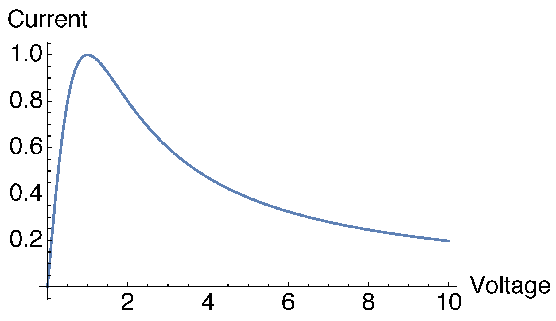
2.4. Current–Voltage Characteristic Curve

For constant current density and field, $n=1$, and solving $J_n=J$ for (31) yields

$$J=\frac{2F}{1+F^2}+O\left({\lambda }^2\right).$$

(32)

Here, J is proportional to the current through the SL and F is proportional to the voltage between its ends. Thus, Equation (32) is the (Esaki–Tsu) current–voltage characteristic curve plotted in Figure 1.

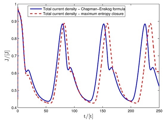
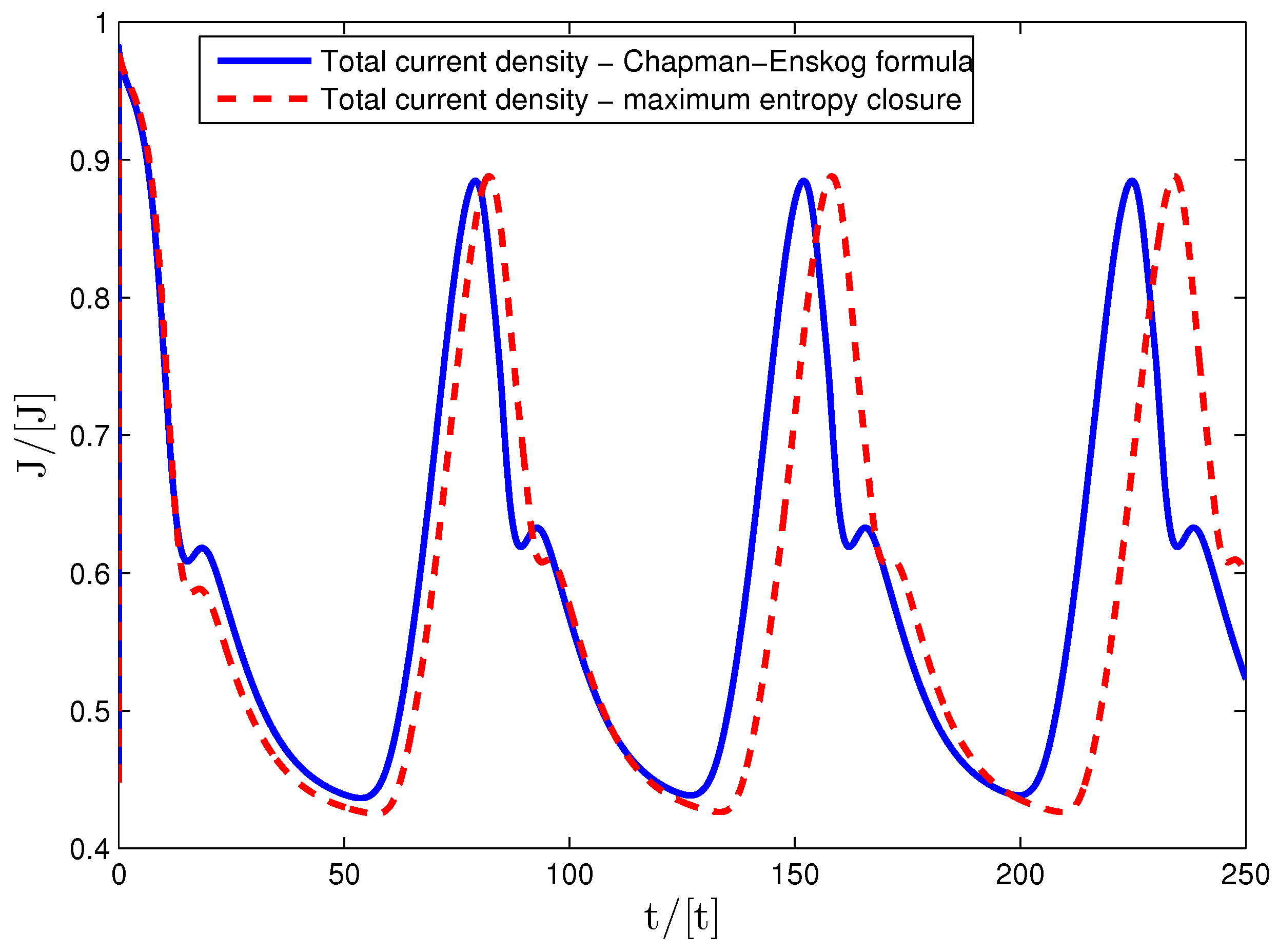
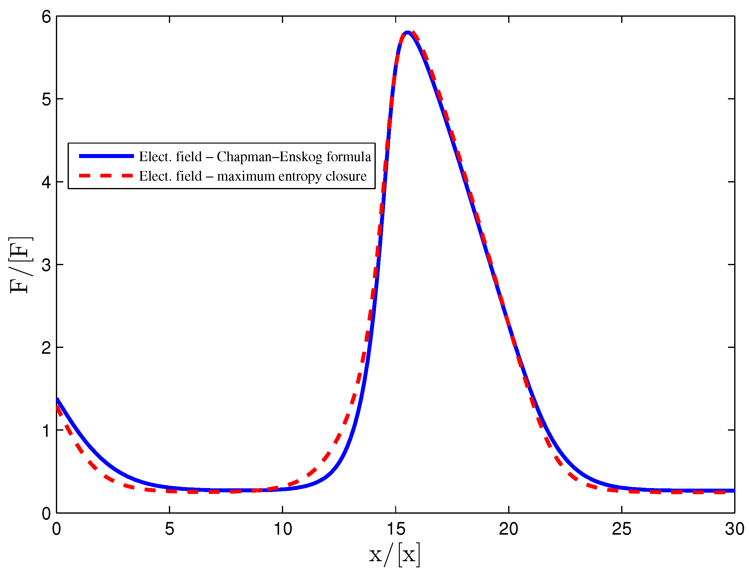
2.5. Comparison to the Chapman–Enskog Result

2.5.1. Chapman–Enskog Formula for the Electron Current Density

In [21], the current density has been obtained by using the Chapman–Enskog perturbation method in the limit as $\lambda \to 0$. The derivation of balance equations from SL Boltzmann–Poisson kinetic equations by the Chapman–Enskog method can be found in [14,16,19,22]. For this perturbation method to work, we need to solve (explicitly, if possible) a reduced kinetic equation containing only dominant balance terms and then we need to find the solvability conditions for a linearized problem about the reduced kinetic equation [14]. In the present case, the Chapman–Enskog ansatz consists of expanding the distribution function and $\partial F/\partial t$ as expansions in powers of the small parameter λ:

$$\begin{array}{c}f(x,k,t;\lambda )=\sum _{m=0}^{\infty }{\psi }^{\left(m\right)}(k;F,n){\lambda }^m,\hfill \end{array}$$

(33)

$$\begin{array}{c}\frac{\partial F}{\partial t}+\sum _{m=0}^{\infty }{\mathcal{J}}^{\left(m\right)}(F,n){\lambda }^m=J\left(t\right).\hfill \end{array}$$

(34)

The functions ${\psi }^{\left(m\right)}(k;F,n)$ are $2\pi$-periodic in k and depend on x and t only through their dependence on the electric field and the electron density (which are related through the Poisson equation). The functionals ${\mathcal{J}}^{\left(m\right)}(F,n)$ should be determined so that the linear equations for ${\psi }^{\left(m\right)}(k;F,n)$ ($m\ge 1$) have bounded solutions that are $2\pi$-periodic in k. Moreover, if we integrate (33) over k and use (7), we find

$$\begin{array}{c}\hfill n={\psi }_0^{\left(0\right)};\frac{1}{2\pi }{\int }_{-\pi }^{\pi }{\psi }^{\left(m\right)}(k;n)dk={\psi }_0^{\left(m\right)}=0,m\ge 1.\end{array}$$

(35)

${\psi }^{\left(0\right)}$ solves Equation (5) for $\lambda =0$,

$$\begin{array}{c}\hfill F\frac{\partial {\psi }^{\left(0\right)}}{\partial k}=-\frac{{\psi }^{\left(0\right)}-f^B}{{\tau }_e}-\frac{{\tau }_e^2-1}{2{\tau }_e}[{\psi }^{\left(0\right)}-{\psi }^{\left(0\right)}(x,-k,t)],\end{array}$$

(36)

which highlights the dominant balance between the collision terms and the field dependent term in the kinetic equation. The solution of (36) is easily found as a Fourier series,

$$\begin{array}{c}\hfill {\psi }^{\left(0\right)}(k;F)=n\sum _{j=-\infty }^{\infty }\frac{(1-ijF/{\tau }_e)I_{j0}}{(1+j^2{F}^2)I_{00}}{e}^{ijk}.\end{array}$$

(37)

Note that the approximate current density, $-\gamma$ Im${\psi }_1^{\left(0\right)}$, coincides with (24). Due to the effect of the electric field, the leading order distribution ${\psi }^{\left(0\right)}$ strongly departs from the local equilibrium distribution $f^B$.

The rest of the Chapman–Enskog expansion terms (${\psi }^{\left(m\right)}$, $m\ge 1$) can be obtained by inserting Equations (33) and (34) into Equation (5) and equating all coefficients of ${\lambda }^m$ in the resulting series to zero. We find the hierarchy:

$$\begin{array}{c}\mathcal{L}{\psi }^{\left(1\right)}=\left.-{\left(\frac{\partial {\psi }^{\left(0\right)}}{\partial t}\right|}_0+\gamma sin\left(k\right)\frac{\partial {\psi }^{\left(0\right)}}{\partial x}\right),\hfill \end{array}$$

(38)

$$\begin{array}{c}\mathcal{L}{\psi }^{\left(2\right)}={\left.\left.-{\left(\frac{\partial {\psi }^{\left(1\right)}}{\partial t}\right|}_0+\gamma sin\left(k\right)\frac{\partial {\psi }^{\left(1\right)}}{\partial x}\right)-\frac{\partial }{\partial t}{\psi }^{\left(0\right)}\right|}_1,\hfill \end{array}$$

(39)

and so on. Here

$$\begin{array}{c}\hfill \mathcal{L}u\left(k\right)\equiv F\frac{\partial u}{\partial k}+\frac{1}{{\tau }_e}\left[\left(\frac{{\tau }_e^2+1}{2}\right)u-\left(\frac{{\tau }_e^2-1}{2}\right)u(-k)\right],\end{array}$$

(40)

and the subscripts 0 and 1 in the RHS of these equations mean that $\partial F/\partial t$ is replaced by $J-{\mathcal{J}}^{\left(0\right)}(F,n)$ and by $-{\mathcal{J}}^{\left(1\right)}(F,n)$, respectively.

The solvability conditions for (38) and (39) are that the zeroth Fourier coefficients (integrals over k) of their RHS vanish. The solvability condition for (38) yields the continuity Equation (13) with $f_1={\psi }_1^{\left(0\right)}$, which holds up to $O\left(\lambda \right)$ terms. Equation (38) yields the first order correction to the distribution Function (37). Let S be the RHS of (38). The solution of (38) has Fourier coefficients

$$\begin{array}{c}\hfill {\psi }_j^{\left(1\right)}(k;F)=\frac{{\tau }_e\mathrm{Re}{S}_j^{\left(1\right)}+i{\tau }_e^{-1}\mathrm{Im}{S}_j^{\left(1\right)}-ijF{S}_j^{\left(1\right)}}{1+j^2{F}^2}.\end{array}$$

(41)

Note that (35) implies that ${\psi }^{\left(1\right)}$ does not contain a contribution proportional to ${\psi }^{\left(0\right)}$. From (37) and (41), we calculate $\mathrm{Im}{\psi }_1^{\left(0\right)}$ and $\mathrm{Im}{\psi }_1^{\left(1\right)}$ and then insert them into the Ampère’s law (34), thereby obtaining the following drift-diffusion equation for the field:

$$\begin{array}{c}\hfill \frac{\partial F}{\partial t}+J_n^{CE}=J\left(t\right),J_n^{CE}={\mathcal{J}}^{\left(0\right)}(F,n)+\lambda {\mathcal{J}}^{\left(1\right)}(F,n)+O\left({\lambda }^2\right),\end{array}$$

(42)

where now the electron current density is:

$$\begin{array}{ccc}\hfill J_n^{CE}& =& \frac{2nF}{1+F^2}-\frac{\lambda }{1+F^2}\left[\frac{2n(1-F^2-2{\tau }_e^2{F}^2)}{{\tau }_e{(1+F^2)}^2}\left(J\left(t\right)-\frac{2nF}{1+F^2}\right)-\frac{4({\tau }_e+{\tau }_e^{-1})F}{1+F^2}\frac{\partial }{\partial x}\left(\frac{nF}{1+F^2}\right)\right.\hfill \\ & +& \left.\frac{{\gamma }^2}{2{\tau }_e}\frac{{\partial }^{2}F}{\partial x^2}-\frac{{\gamma }^2{I}_{20}}{2{\tau }_e{I}_{00}}\frac{\partial }{\partial x}\left(\frac{n}{1+4F^2}\right)+\frac{{\gamma }^2{I}_{20}F}{{\tau }_e{I}_{00}}\frac{\partial }{\partial x}\left(\frac{nF}{1+4F^2}\right)\right]+O\left({\lambda }^2\right).\hfill \end{array}$$

(43)

Equation (43) coincides with (32) of [21] when $f_j^{FD}$ in the latter is approximated by the result of using a Boltzmann local equilibrium distribution, $n{I}_{j0}/I_{00}$.

The difference between the electron current density (31), given by maximum entropy closure, and (43), given by the Chapman–Enskog method, is of order λ, more precisely,

$$\begin{array}{ccc}\hfill J_n^{CE}-J_n^{ME}& =& -\frac{\lambda }{1+F^2}\left[\frac{{\gamma }^2{I}_2}{2{\tau }_e{I}_0}\frac{{\partial }^{2}F}{\partial x^2}-\frac{{\gamma }^2{I}_{20}}{2{\tau }_e{I}_{00}}\frac{\partial }{\partial x}\left(\frac{n}{1+4F^2}\right)+\frac{{\gamma }^2{I}_{20}F}{{\tau }_e{I}_{00}}\frac{\partial }{\partial x}\left(\frac{nF}{1+4F^2}\right)\right.\hfill \\ & -& \left.\frac{2\gamma nF}{\frac{{(1+F^2)}^2}{2}\left(1+\frac{I_2}{I_0}\right)-\frac{I_{10}^2}{I_{00}^2}}\left(\frac{1}{2}+\frac{I_3}{2I_0}-\frac{4{\tau }_e^2}{{\gamma }^2{(1+F^2)}^2}\right)\frac{\partial F}{\partial x}\right]+O\left({\lambda }^2\right).\hfill \end{array}$$

(44)

Note that $J_n^{CE}=J_n^{ME}$ for constant values of current density and field. Thus, up to $O\left({\lambda }^2\right)$ terms, the current–voltage characteristic curve for uniform field is that depicted in Figure 1, no matter whether we use the Chapman–Enskog formula or maximum entropy closure to calculate it.

2.5.2. Boundary and Initial Conditions

To solve the balance Equations (6), (20) and (31) or Equation (43), we need boundary and initial conditions. We will use the following nondimensional Ohmic boundary conditions at the contacts, [19,21]:

$$\begin{array}{c}\frac{\partial F(0,t)}{\partial t}+\sigma F(0,t)=J\left(t\right)\hfill \end{array}$$

(45)

$$\begin{array}{c}n(L,t)=1\hfill \end{array}$$

(46)

where $\sigma >0$ is the constant contact conductivity. The nondimensional voltage bias condition is:

$$\begin{array}{c}{\int }_0^{L}F(x,t)dx=\varphi L,\hfill \end{array}$$

(47)

where $\varphi$ is a nondimensional average electric field and $\varphi L$ the nondimensional voltage. As initial condition for the field, we will use [21]

$$F(x,0)=\varphi .$$

(48)

2.5.3. Numerical Methods

To solve the balance equations, we have used the implicit finite difference method described in [21]. Reference [23] contains a proof of convergence for coupled balance-Poisson equations having the integral voltage bias constraint (47). The idea is to rewrite (20) as

$$\frac{\partial F}{\partial t}+\mathcal{A}\frac{\partial F}{\partial x}+\mathcal{B}\frac{{\partial }^{2}F}{\partial x^2}+\mathcal{C}J\left(t\right)=\mathcal{D}$$

(49)

(where the coefficients $\mathcal{A}$–$\mathcal{D}$ are indicated in [21]), use finite differences (central finite differences for derivatives with respect to x, Simpson’s composite rule for the integral bias condition, and an implicit Euler method for $\partial F/\partial t$), and then reduce the system to inverting a tridiagonal matrix [21]. For the maximum entropy closure, we solve Equation (27) for the Lagrange multiplier β by the Newton method at each time step. The convergence thereof is exceedingly fast.

3. Numerical Results

In previous works [21], we have shown that the balance equations obtained by using the Chapman–Enskog method provide an excellent approximation to the kinetic Boltzmann–Poisson system of equations for realistic parameter values appearing in experiments [20]. In this paper, we adopt the numerical values of parameters and scales as indicated in Table 1, which produce the largest value of the scaling parameter λ found in Schomburg et al’s experiments [20].

To solve numerically the balance equation, we set a voltage within the interval for which there is an asymptotically stable time-dependent solution. As maximum entropy and Chapman–Enskog formulas give the same current–voltage characteristic curve for uniform fields, a comparison of oscillatory solutions seems more appropriate to highlight differences between both formulations. Each oscillation period of the current density corresponds to the generation of an electric field pulse at the emitter contact $x=0$, its motion towards and annihilation at the receiving contact $x=L$ [16,19]. The nondimensional parameter λ is relatively large, $\lambda =0.15$, so as to appreciate the differences between the results of numerically solving the balance equation obtained using the consistent Chapman–Enskog perturbation procedure and the maximum entropy closure. The Chapman–Enskog procedure yields an excellent approximation to the numerical solution of the Boltzmann–Poisson equation, as shown in [21]. Figure 2 shows that the maximum entropy closure produces a slightly larger oscillation period which results in the observed shift. The corresponding oscillation frequencies are 31 GHz (maximum entropy) and 32.3 GHz (Chapman–Enskog), which result in a 0.04 (4%) relative error. This is quite small compared with the perturbation parameter $\lambda =0.15$ that measures the differences between both approximations.

Figure 3 compares the electric field profile at the same time within an oscillation period for the solutions obtained using maximum entropy and the Chapman–Enskog procedure. This instant corresponds to having a fully developed field pulse far from the contacts and, as the periods of both numerical approximations are slightly different, the times have been appropriately shifted. We observe that the field maximum is the same in both cases.

4. Discussion and Conclusions

We have shown how to derive macroscopic balance equations for the electric field and the electron density for nonlinear charge transport in SLs by combining the maximum entropy closure of moment equations and a simple perturbation expansion that holds in the limit as the Bloch frequency, $e{F}_{M}l$, and the collision frequency ${\nu }_{en}{\tau }_e$ are of the same order and dominate all other terms in the kinetic equation. In this situation, the distribution function is far from the local equilibrium distribution $f^B$ of (8). In turn, our local equilibrium depends on the instantaneous electron density and therefore it is far from global thermodynamic equilibrium. Then it is far from obvious whether a closure based on the minimum entropy production principle (that holds for linear kinetic equations close to global equilibrium) is possible [13].

We have found that the maximum entropy balance equations for electron density and electric field agree with those derived by the systematic Chapman–Enskog perturbation method up to small convective and diffusive terms. These terms depend on gradients of the field or the electron density and therefore vanish for uniform fields. Therefore the uniform stationary current–voltage characteristic curve is the same whether calculated by maximum entropy or Chapman–Enskog formulas. For a long superlattice and DC voltages below a certain critical value, the solution of the balance equations is stationary and almost uniform [16]. Thus its current–voltage characteristic curve follows that of Figure 1 up to the critical voltage (located on the low-voltage increasing part of Figure 1). For larger voltage bias, the balance equations have stable time periodic solutions. These oscillatory solutions are due to the repeated creation and motion of electric field pulses at the injecting contact [16] and, because of the pulses’ large spatial gradients, we surmise that differences between maximum entropy and Chapman–Enskog formulations are more pronounced in the oscillatory case. In our simulations, we have used the parameter values corresponding to the superlattice in Schomburg et al’s experiments [20] that yields the largest dimensionless expansion parameter λ used in perturbation theory. A numerical simulation shows that the differences in oscillation frequency are smaller than the dimensionless expansion parameter λ. As the Chapman–Enskog procedure gives an excellent approximation to the solution of the Boltzmann–Poisson kinetic theory equations even for that value of λ [21], our results show that the maximum entropy closure also produces a very good numerical approximation. From the computational point of view, the maximum entropy closure is somewhat costlier in that the Lagrange multiplier(s) need to be calculated numerically at each step or at once in a table of values. However, the maximum entropy closure can be used in cases where there is not a clear expansion procedure to reduce the kinetic equation to a much less costly balance equation.

Recapitulating, we have studied a DC voltage biased miniband semiconductor superlattice in conditions very far from global equilibrium. This nanoelectronic system is described by a Boltzmann–Poisson system of equations with a simplified collision kernel that includes relaxation to a local equilibrium dependent on the instantaneous value of the electron density. The device is an open system connected to injecting and receiving contacts. We have compared the numerical solutions of balance equations obtained from maximum entropy closure and from a Chapman–Enskog perturbation procedure in the hyperbolic limit of strong electric fields. We have found the same stationary uniform current–voltage characteristic curve with both procedures. For large voltages, there are stable time periodic solutions of the balance equations due to periodic formation of pulses at the injecting contact that move toward the receiving contact. Even in this case of large spatial gradients, the maximum entropy closure provides numerical solutions that are very close to those obtained from the Chapman–Enskog formulation. Thus the maximum entropy closure is a good option that may be applicable even in cases in which there is no viable perturbation procedure to derive balance equations.

There are interesting research directions to extend this investigation. It is simple to extend our results to a SL with a Fermi–Dirac local equilibrium distribution as in [19]. In this case, there are two Lagrange multipliers in the local equilibrium that need to be calculated: β and a chemical potential that is a function of the electron density and of the energy density. We have to solve two algebraic relations instead of one, which make solving balance equations most costly. See Appendix A.

Another problem in which a combination of maximum entropy closure and hyperbolic limit could provide interesting results is that of a hydrodynamic description of Bloch oscillations in a wide miniband SL [22]. In this case, the maximum entropy principle can also give a second harmonic $f_2$ that closes the moment equation for $f_1$. The theory is more complicated as $f_1$ may oscillate with time at a high Bloch frequency and have a stationary or an oscillatory envelope, as explained in [22]. See Appendix B for the appropriate maximum entropy distribution.

In many other problems, it is not possible to do similar comparisons of maximum entropy and perturbation closures because a solution of the kinetic equation for the high field and strong collision limit is not known [6,7,8,9,24,25]. Changing the collision operator so that it has relaxation time form [26] may allow a comparison similar to that in the present paper.

There are no known systematic perturbation methods capable to derive hydrodynamic balance equations from quantum kinetic equations with realistic collision kernels, such as nonequilibrium Green functions [15,27]. For example, the Chapman–Enskog method works for quantum Wigner-Poisson equations provided a very simplified collision kernel is used, see [28,29,30]. In principle, the maximum entropy closure should work for such quantum kinetic equations although this research venue is insufficiently explored.

References

1. Tribus, M.; Levine, R.D. The Maximum Entropy Formalism; MIT Press: Cambridge, MA, USA, 1978. [Google Scholar]
2. Zwanzig, R. Nonequilibrium Statistical Mechanics; Oxford University Press: Oxford, UK, 2001. [Google Scholar]
3. Levermore, C.D. Moment Closure Hierarchies for Kinetic Theories. J. Stat. Phys. 1996, 83, 1021–1065. [Google Scholar] [CrossRef]
4. Anile, A.M.; Romano, V. Non parabolic band transport in semiconductors: Closure of the moment equations. Contin. Mech. Thermodyn. 1999, 11, 307–325. [Google Scholar] [CrossRef]
5. Anile, A.M.; Muscato, O.; Romano, V. Moment equations with maximum entropy closure for carrier transport in semiconductor devices: Validation in bulk silicon. VLSI Des. 2000, 10, 335–354. [Google Scholar] [CrossRef]
6. Degond, P.; Ringhofer, C. Quantum moment hydrodynamics and the entropy principle. J. Stat. Phys. 2003, 112, 587–628. [Google Scholar] [CrossRef]
7. Romano, V. Quantum corrections to the semiclassical hydrodynamical model of semiconductors based on the maximum entropy principle. J. Math. Phys. 2007, 48, 123504. [Google Scholar] [CrossRef]
8. Degond, P.; Gallego, S.; Méhats, F.; Ringhofer, C. Quantum hydrodynamic and diffusion models derived from the entropy principle. In Quantum Transport: Modelling, Analysis and Asymptotics; Ben Abdallah, N., Frosali, G., Eds.; Springer: Berlin/Heidelberg, Germany, 2008; Volume 1946, pp. 111–168. [Google Scholar]
9. Camiola, V.D.; Romano, V. 2DEG-3DEG charge transport model for MOSFET based on the Maximum Entropy Principle. SIAM J. Appl. Math. 2013, 73, 1439–1459. [Google Scholar] [CrossRef]
10. Prigogine, I. Étude Thermodynamique des Phénomènes Irréversibles; Dunod: Brussel, Belgium, 1947. (In French) [Google Scholar]
11. Klein, M.J.; Meijer, P.H.E. Principle of minimum entropy production. Phys. Rev. 1954, 96, 250–255. [Google Scholar] [CrossRef]
12. De Groot, S.; Mazur, P. Non-Equilibrium Thermodynamics; Dover: New York, NY, USA, 1984. [Google Scholar]
13. Christen, T.; Kassubek, F. Entropy production moment closures and effective transport coefficients. J. Phys. D Appl. Phys. 2014, 47, 363001. [Google Scholar] [CrossRef]
14. Bonilla, L.L.; Teitsworth, S.W. Nonlinear Wave Methods for Charge Transport; Wiley-VCH: Weinheim, Germany, 2010. [Google Scholar]
15. Wacker, A. Semiconductor superlattices: A model system for nonlinear transport. Phys. Rep. 2002, 357. [Google Scholar] [CrossRef]
16. Bonilla, L.L.; Grahn, H.T. Nonlinear dynamics of semiconductor superlattices. Rep. Prog. Phys. 2005, 68, 577–683. [Google Scholar] [CrossRef]
17. Ktitorov, S.A.; Simin, G.S.; Sindalovskii, Y.V. Bragg reflections and the high-frequency conductivity of an electronic solid-state plasma. Sov. Phys. Solid State 1972, 13, 1872–1874. [Google Scholar]
18. Ignatov, A.A.; Shashkin, V.I. Bloch oscillations of electrons and instability of space-charge waves in semiconductor superlattices. Sov. Phys. JETP 1987, 66, 526–530. [Google Scholar]
19. Bonilla, L.L.; Escobedo, R.; Perales, A. Generalized drift-diffusion model for miniband superlattices. Phys. Rev. B 2003, 68, 241304. [Google Scholar] [CrossRef]
20. Schomburg, E.; Blomeier, T.; Hofbeck, K.; Grenzer, J.; Brandl, S.; Ignatov, A.A.; Renk, K.F.; Pavel’ev, D.G.; Koschurinov, Yu.; Melzer, B.Y.; et al. Current oscillation in superlattices with different miniband widths. Phys. Rev. B 1998, 58, 4035–4038. [Google Scholar] [CrossRef]
21. Alvaro, M.; Cebrián, E.; Carretero, M.; Bonilla, L.L. Numerical methods for kinetic equations in semiconductor superlattices. Comput. Phys. Commun. 2013, 184, 720–731. [Google Scholar] [CrossRef]
22. Bonilla, L.L.; Alvaro, M.; Carretero, M. Theory of spatially inhomogeneous Bloch oscillations in semiconductor superlattices. Phys. Rev. B 2011, 84, 155316. [Google Scholar] [CrossRef]
23. Carpio, A.; Hernando, P.J.; Kindelan, M. Numerical study of hyperbolic equations with integral constraints arising in semiconductor theory. SIAM J. Numer. Anal. 2001, 39, 168–191. [Google Scholar] [CrossRef]
24. Lichtenberger, P.; Morandi, O.; Schürrer, F. High-field transport and optical phonon scattering in graphene. Phys. Rev. B 2011, 84, 045406. [Google Scholar] [CrossRef]
25. Camiola, V.D.; Romano, V. Hydrodynamical Model for Charge Transport in Graphene. J. Stat. Phys. 2014, 157, 1114–1137. [Google Scholar] [CrossRef]
26. Bonilla, L.L.; Alvaro, M.; Carretero, M.; Sherman, E.Y. Dynamics of optically injected currents in carbon nanotubes. Phys. Rev. B 2014, 90, 165441. [Google Scholar] [CrossRef]
27. Freericks, J.K. Transport in Multilayered Nanostructures; Imperial College Press: London, UK, 2006. [Google Scholar]
28. Bonilla, L.L.; Escobedo, R. Wigner–Poisson and nonlocal drift-diffusion model equations for semiconductor superlattices. Math. Models Methods Appl. Sci. 2005, 15, 1253–1272. [Google Scholar] [CrossRef]
29. Bonilla, L.L.; Barletti, L.; Alvaro, M. Nonlinear electron and spin transport in semiconductor superlattices. SIAM J. Appl. Math. 2008, 69, 494–513. [Google Scholar] [CrossRef]
30. Alvaro, M.; Bonilla, L.L. Two mini-band model for self-sustained oscillations of the current through resonant tunneling semiconductor superlattices. Phys. Rev. B 2010, 82, 035305. [Google Scholar] [CrossRef]
Figure 1. Nondimensional current–voltage characteristic curve J ( F ) for constant field and current density. Up to order λ 2 terms, it is the same whether we use maximum entropy closure or the Chapman–Enskog formula derived below.
Entropy 18 00260 g001
Figure 2. Nondimensional current density versus time from the current balance equation obtained by using the Chapman–Enskog (solid line) and the maximum entropy closure (dashed line). Current density and time scales are as in Table 1 for a DC voltage bias of 1.5312 V.
Entropy 18 00260 g002
Figure 3. Nondimensional field profile at the same instant of an oscillation period from the current balance equation obtained by using the Chapman–Enskog (solid line) and the maximum entropy closure (dashed line). Field and space scales are as in Table 1 for a DC voltage bias of 1.5312 V.
Entropy 18 00260 g003