Efficiency of Harmonic Quantum Otto Engines at Maximal Power


Department of Physics, University of Maryland Baltimore County, Baltimore, MD 21250, USA
Entropy 2018, 20(11), 875; https://0-doi-org.brum.beds.ac.uk/10.3390/e20110875
Submission received: 24 October 2018
/
Revised: 10 November 2018
/
Accepted: 13 November 2018
/
Published: 15 November 2018
(This article belongs to the Special Issue Fluctuation Relations and Nonequilibrium Thermodynamics in Classical and Quantum Systems)
Abstract
:Recent experimental breakthroughs produced the first nano heat engines that have the potential to harness quantum resources. An instrumental question is how their performance measures up against the efficiency of classical engines. For single ion engines undergoing quantum Otto cycles it has been found that the efficiency at maximal power is given by the Curzon–Ahlborn efficiency. This is rather remarkable as the Curzon–Alhbron efficiency was originally derived for endoreversible Carnot cycles. Here, we analyze two examples of endoreversible Otto engines within the same conceptual framework as Curzon and Ahlborn’s original treatment. We find that for endoreversible Otto cycles in classical harmonic oscillators the efficiency at maximal power is, indeed, given by the Curzon–Ahlborn efficiency. However, we also find that the efficiency of Otto engines made of quantum harmonic oscillators is significantly larger.
1. Introdcution
It is a standard exercise of thermodynamics to compute the efficiency of engines, i.e., to determine the relative work output for devices undergoing cyclic transformations on the thermodynamic manifold [1]. Like few other applications the study of heat engines illustrates the versatility of thermodynamic concepts, since universally valid bounds can be obtained purely from macroscopic, phenomenological knowledge about physical systems. However, all ideal cycles, such as the Carnot, Stirling, Otto, Diesel, etc. cycles are only of limited practical importance, as they are comprised of quasistatic, infinitely slow state transformations. Therefore, the power output of an ideal engine is strictly zero [1].
All real engines operate in finite time, and thus their working medium is almost never in equilibrium with the environment. Moreover, a more practical question is to determine the efficiency at maximal power output, rather than focusing only at the ideal, maximal efficiency (at zero power). In a seminal paper [2], Curzon and Ahlborn tackled this problem within the framework of endoreversible thermodynamics [3].
At the core of endoreversible thermodynamics is the idea of local equilibrium: Imagine an engine, whose working medium is in a state of thermal equilibrium of temperature T. However, T is not equal to the temperature of the environment, , and thus there is a temperature gradient at the boundaries of the engine. One then studies the engine as it slowly undergoes a cyclic state transformation, where slow means that the working medium remains locally in equilibrium at all times. However, since the cycle does operate in finite time, the working medium never fully equilibrates with the environment. Therefore, from the point of view of the environment the device undergoes an irreversible cycle. Such state transformations are called endoreversible [3], which means that locally the transformation is reversible, but globally irreversible.
Curzon and Ahlborn showed [2] that the efficiency of a Carnot engine undergoing an endoreversible cycle at maximal power is given by,
where and are the temperatures of the cold and hot reservoirs, respectively. Remarkably, it has been found that (1) is also assumed by many, physically different engines at maximal power, such as an endoreversible Otto engine with an ideal gas as working medium [4], the endoreversible Stirling cycle [5], Otto engines in open quantum systems in the quasistatic limit [6], or a single ion in a harmonic trap undergoing a quantum Otto cycle [7,8]. On the other hand, it also has been shown that whether or not a finite time Carnot cycle assumes is determined by the “symmetry” of dissipation [9], and the efficiency of an Otto engine working with a single Brownian particle in a harmonic trap is determined by the specific parameterization of the trap’s stiffness [10].
In particular, the recent experimental breakthroughs in the implementation of nanosized heat engines [11,12] that could principally exploit quantum resources [13,14,15,16,17,18,19,20,21,22,23,24] pose the question whether their behavior can be universally characterized. For instance, Reference [6] suggested that to describe the efficiency at maximal power could be such a universal result, at least for a class of engines. However, the Curzon–Ahlborn efficiency (1) was originally derived for endoreversible Carnot cycles, which is independent on the nature of the working medium. On the other hand, a standard textbook exercise shows that the Otto efficiency is dependent on the equation of state, i.e., on the specific working medium [1]. Therefore, it would actually be more natural to expect that the efficiency at maximal power strongly depends on the nature of working medium. Similar conclusions have been drawn, for instance, in the thermodynamic analysis of photovolatic cells [25,26,27].
In addition, the quantum Otto cycle is typically comprised of two thermalization and two unitary strokes [28,29,30]. For cycles involving only unitary strokes [7,8] the assumption of local equilibrium is almost never justified, and thus it becomes even more remarkable that at maximal power output a quantum Otto cycle in a parametric, harmonic oscillator operates with the Curzon–Ahlborn efficiency [7,8]. Also see Reference [6] for a more detailed treatment from open quantum dynamics. Therefore, the question arises whether this is a peculiarity of the quantum Otto cycle in the harmonic oscillator, or whether there is something more fundamental and universal about .
The purpose of the present work is to revisit these longstanding questions and study the endoreversible Otto cycle in a conceptually simple and pedagogical approach similar to Curzon and Ahlborn’s original treatment [2]. To this end, we compute the efficiency at maximal power for two examples of endoreversible Otto engines. We start with a classical version, for which the working medium is a single Brownian particle in a harmonic trap. Maximizing the power output with respect to the compression ratio, we find analytically that the efficiency is indeed given by (1). As a second example we study a quantum engine, whose working medium is a quantum harmonic oscillator ultraweakly coupled to the thermal environment. We find that in this case the efficiency is larger than (1), which demonstrates that the Curzon–Ahlborn efficiency is not universal at maximal power. An advantage of the present treatment is that it is somewhat more pedagogical than earlier works on the topic. The present derivation is entirely based on the phenomenological framework of endoreversible thermodynamics. Thus, e.g., neither the full quantum dynamics [6] nor the linear response problem [10] have to be solved.
2. Carnot Engine at Maximal Power
We begin by briefly reviewing the main gist of Reference [2] and by establishing notions and notation. In particular, we focus on the limits and assumptions that lead to the Curzon–Ahlborn efficiency (1) for endoreversible Carnot engines.
The ideal Carnot cycle consists of two isothermal processes during which the systems absorbs/exhausts heat and two thermodynamically adiabatic, i.e., isentropic strokes [1]. During the isentropic strokes the working medium does not exchange heat with the thermal reservoirs, and thus its state can be considered to be independent of the environment. Therefore, we only have to modify the treatment of the isothermal strokes during which the working medium will be in a local equilibrium state at different temperature than the temperature of the hot and cold reservoir, respectively.
In particular, during the hot isotherm the working medium is assumed to be a little cooler than the hot environment at . Thus, during the whole stroke the system absorbs the heat
where is the stroke time, is the temperature of the working medium, and is a constant depending on thickness and thermal conductivity of the boundary separating working medium and environment. Note that Equation (2) is nothing else but a discretized version of Fourier’s law for heat conduction [1]. We will see shortly that for Otto cycles the rate of heat flux can no longer be assumed to be constant, since we need to account for the change in temperature during the isochoric strokes.
Similarly, during the cold isotherm the system is a little warmer than the cold reservoir at . Hence, the exhausted heat can be written as
where is the cold heat transfer coefficient.
As mentioned above, the adiabatic strokes are unmodified, but note that the cycle is taken to be reversible with respect to the local temperatures of the working medium. Hence, we can write
Equation (4) allows to relate the stroke times and to the heat transfer coefficients and .
We are now interested in determining the efficiency at maximal power. To this end, we write the power output of the cycle as
where and . In Equation (5) we introduced the total cycle time , and thus . Note that this neglects any explicit dependence of the analysis on the lengths of the adiabatic strokes. We exclusively focus on the isotherms, i.e, on the temperature differences between working medium and the hot and cold reservoirs.
It is worth emphasizing that in the present problem we have four free parameters, namely hot and cold temperatures of the working substance, and , and the stroke times and . The balance equation for the entropy (4) allows to eliminate two of these, and Curzon and Ahlborn chose to eliminate and [2].
Thus, we maximize the power as a function of the difference in temperatures between working substance and environment. After a few lines of algebra one obtains [2],
where the maximum is assumed for
From these expressions we can now compute the efficiency. We have,
where we used Equation (4). Thus, the efficiency of an endoreversible Carnot cycle at maximal power output becomes
which only depends on the temperatures of the hot and cold reservoirs.
In the following, we will apply exactly the same reasoning to the endoreversible Otto cycle.
3. Endoreversible Otto Cycle
The standard Otto cycle is a four-stroke cycle consisting of isentropic compression, isochoric heating, isentropic expansion, and ischoric cooling [1]. Thus, we have in the endoreversible regime:
3.1. Isentropic Compression
During the isentropic strokes the working substance does not exchange heat with the environment. Therefore, the thermodynamic state of the working substance can be considered independent of the environment, and the endoreversible description is identical to the equilibrium cycle. From the first law of thermodynamics, , we have,
where is the heat exchanged, and is the work performed during the compression. Moreover, denotes the work parameter, such as the inverse volume of a piston or the frequency of a harmonic oscillator (20).
3.2. Isochoric Heating
During the isochoric strokes the work parameter is held constant, and the system exchanges heat with the environment. Thus, we have for isochoric heating
In complete analogy to Curzon and Ahlborn’s original analysis [2] we now assume that the working substance is in a state of local equilibrium, but also that the working substance never fully equilibrates with the hot reservoir. Therefore, we can write
where as before is the duration of the stroke.
Note that in contrast to the Carnot cycle the Otto cycle does not involve isothermal strokes, and, hence, the rate of heat flux is not constant. Rather, we have to explicitly account for the change in temperature from to . To this end, Equation (2) is replaced by Fourier’s law [1],
where is a constant depending on the heat conductivity and heat capacity of the working substance.
Equation (13) can be solved exactly, and we obtain the relation
In the following, we will see that Equation (14) is instrumental in reducing the number of free parameters.
3.3. Isentropic Expansion
In complete analogy to the compression, we have for the isentropic expansion,
3.4. Isochoric Cooling
Heat and work during the isochoric cooling read,
where we now have
4. Classical Harmonic Engine
To continue the analysis we now need to specify the internal energy E. As a first example, we consider a classical Brownian particle trapped in a harmonic oscillator. The bare Hamiltonian reads,
where m is the mass of the particle.
For a particle in thermal equilibrium the Gibbs entropy, S, and the internal energy, E, are
where we introduced Boltzmann’s constant, .
Note, that from Equation (21) we obtain a relation between the frequencies, and and the four temperatures, , , , and . To this end, consider the isentropic strokes, for which we have
which is fulfilled by
We are now equipped with all the ingredients necessary to compute the endoreversible efficiency,
In complete analogy to fully reversible cycles [1], Equation (24) can be written as
where we used the explicit from of the internal energy E (21). Further, using Equations (23) the endoreversible Otto efficiency becomes
which defines the compression ratio, . Observe that the endoreversible efficiency takes the same form as its reversible counter part [1]. However, in Equation (25) the temperatures correspond the local equilibrium state of the working substance, and not to a global equilibrium with the environment.
Similarly to Curzon and Ahlborn’s treatment of the endoreversible Carnot cycle [2] we now compute the efficiency for a value of , at which the power (5) is maximal. We begin by re-writing the total work with the help of the compression ratio and Equations (23) as,
Further using Equation (14) we obtain
which only depends on the free parameters , , and . Of these three, we can eliminate one more, by combing Equations (14) and (19), and we have
Finally, the power output (5) takes the form,
Remarkably the power output, , factorizes into a contribution that only depends on the compression ratio, , and another term that is governed by the stroke times, and ,
It is then a simple exercise to show that is maximized for any value of and if we have,
Therefore, the efficiency at maximal power reads,
In conclusion, we have shown that for the classical harmonic oscillator the efficiency at maximal power of an endoreversible Otto cycle (24) is indeed given by the Curzon–Ahlborn efficiency (1).
It is worth emphasizing that for the endoreversible Otto cycle we started with six free parameters, the four temperatures , , , and , and the two stroke times, and . Of these, we succeeded in eliminating three, by explicitly using Fourier’s law for the heat transfer, Equations (13) and (18), and the explicit expressions for the entropy and the internal energy (21). Therefore, one would not expect to obtain the same result (33) for other working substances such as the quantum harmonic oscillator.
5. Quantum Harmonic Engine
For the remainder of this analysis we will be interested in a quantum harmonic oscillator in the ultraweak coupling limit [31]. In this limit, a “small” quantum system interacts only weakly with a large Markovian heat bath, such that the stationary state is given by a thermal equilibrium distribution. This situation is similar to the model studied in Reference [6], however in the present case we will not have to solve the full quantum dynamics.
The equilibrium state is given by a Gibbs state, , where is the density operator. Accordingly, the internal energy reads
and the entropy becomes
Despite the functional form of S being more involved, we notice that the four temperatures and the two frequencies are still related by the same Equation (23). Thus, it can be shown [6] that the efficiency of an endoreversible Otto cycle in a quantum harmonic oscillators also reads,
Following the analogous steps that led to Equation (30) we obtain for the power output of an endoreversible quantum Otto engine,
where we set . We immediately observe that in contrast to the classical case (30) the expression no longer factorizes. Consequently, the value of , for which P is maximal does depend on the stroke times and .
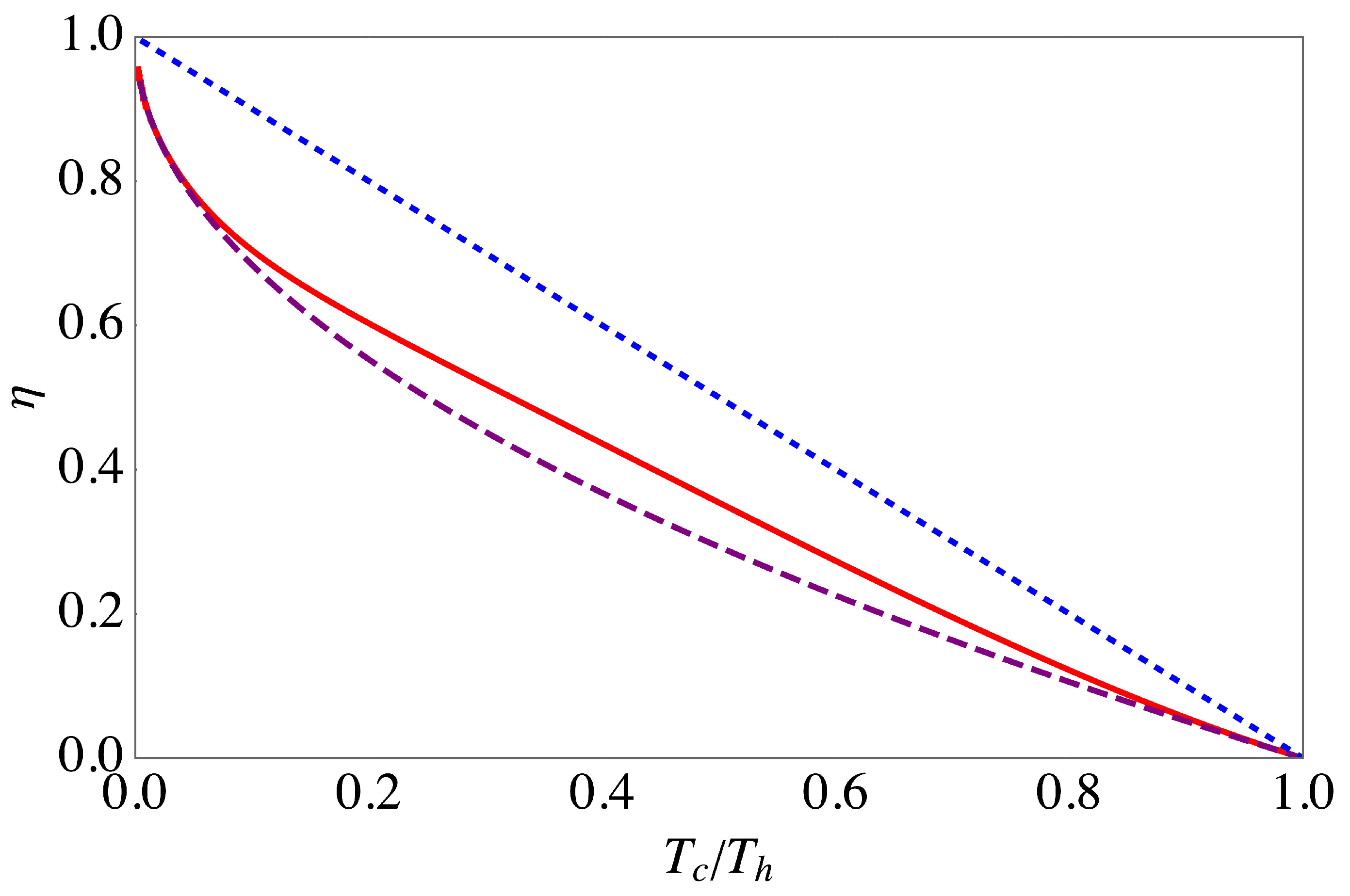
Due to the somewhat cumbersome expression (37) we chose to find the maximum of numerically. In Figure 1 we illustrate our findings in the high temperature limit, . Consistently with our classical example, the efficiency is given by Equation (33), which was also found in Reference [6] for quasistatic cycles. It is worth emphasizing that Figure 1 was obtained numerically for a specific choice of parameters. However, the above, classical analysis revealed that in the limit of high temperatures the result, namely that the efficiency at maximal power is given by the Curzon–Ahlborn efficiency (33), becomes independent of all parameters but the temperatures of the hot and cold reservoirs.
Figure 2 depicts the efficiency at maximal power (36) as a function of in the deep quantum regime, . In this case, we find that the quantum efficiency is larger than the Curzon–Ahlborn efficiency (33). From a thermodynamics’ point-of-view this finding is not really surprising since already in reversible cycles the efficiency strongly depends on the equation of state.
In conclusion, we have shown explicitly that contrary to anecdotal evidence in the literature [4,6,7,8,12] the efficiency at maximal power is not universally given by the Curzon–Ahlborn efficiency—not even for the harmonic oscillator. The natural question now is if and how this “quantum supremacy” can be exploited in the design and experimental implementation of nano engines. This, however, we leave for future work.
6. Concluding Remarks
In the present work we have computed the efficiency at maximal power for two examples of the endoreversible Otto engine. We have found that in the case of a classical harmonic oscillator the efficiency is identical to the Curzon–Ahlborn expression originally found for endoreversible Carnot cycles. However, we have also shown that for engines operating with quantum harmonic oscillators the efficiency significantly differs from the classical expression. These findings are consistent with References [6,10], where it was argued that the efficiency should be governed by internal friction and specific driving protocols, respectively. The advantage of the present analysis is, however, that our results were obtained entirely from the phenomenological equations of endoreversible thermodynamics. Neither the quantum master equation [6] nor the linear response problem [10] had to be solved explicitly.
Finally, we note that the present conclusions are a consequence of the differing equations of state for the classical and quantum harmonic oscillator. More precisely, the maximal power output is governed by the different expressions for the internal energies. As such, the conclusions drawn in this work are more “thermodynamical” as they are “quantum”. By this we mean, that it is entirely possible to find classical working substances, for which the efficiency at maximal power is not given by the Curzon–Ahlborn efficiency. We also have not excluded the existence of other quantum working substance, for which are described by the Curzon–Ahlborn efficiency. However, the hunt for these systems we also leave for future work.
Funding
S.D. acknowledges support from the U.S. National Science Foundation under Grant No. CHE-1648973.
Acknowledgments
It is a pleasure to thank Gregory Huxtable for enjoyable discussions during an early stage of this project, and Steve Campbell, Obinna Abah, and Marcus V. S. Bonança for many years of fruitful exchange of ideas.
Conflicts of Interest
The author declares no conflict of interest.
References
- Callen, H. Thermodynamics and an Introduction to Thermostastistics; Wiley: New York, NY, USA, 1985. [Google Scholar]
- Curzon, F.L.; Ahlborn, B. Efficiency of a Carnot engine at maximum power output. Am. J. Phys. 1975, 43, 22–24. [Google Scholar] [CrossRef]
- Hoffmann, K.H.; Burzler, J.M.; Schubert, S. Endoreversible thermodynamics. J. Non-Equilib. Thermodyn. 1997, 22, 311–355. [Google Scholar] [CrossRef]
- Leff, H.S. Thermal efficiency at maximum work output: New results for old heat engines. Am. J. Phys. 1987, 55, 602–610. [Google Scholar] [CrossRef]
- Erbay, L.B.; Yavuz, H. Analysis of the Stirling heat engine at maximum power conditions. Energy 1997, 22, 645–650. [Google Scholar] [CrossRef]
- Rezek, Y.; Kosloff, R. Irreversible performance of a quantum harmonic heat engine. New J. Phys. 2006, 8, 83. [Google Scholar] [CrossRef]
- Abah, O.; Roßnagel, J.; Jacob, G.; Deffner, S.; Schmidt-Kaler, F.; Singer, K.; Lutz, E. Single-Ion Heat Engine at Maximum Power. Phys. Rev. Lett. 2012, 109, 203006. [Google Scholar] [CrossRef] [PubMed]
- Roßnagel, J.; Abah, O.; Schmidt-Kaler, F.; Singer, K.; Lutz, E. Nanoscale Heat Engine Beyond the Carnot Limit. Phys. Rev. Lett. 2014, 112, 030602. [Google Scholar] [CrossRef] [PubMed]
- Esposito, M.; Kawai, R.; Lindenberg, K.; Van den Broeck, C. Efficiency at Maximum Power of Low-Dissipation Carnot Engines. Phys. Rev. Lett. 2010, 105, 150603. [Google Scholar] [CrossRef] [PubMed]
- Bonança, M.V.S. Approaching Carnot efficiency at maximum power in linear response regime. arXiv, 2018; arXiv:1809.09163. [Google Scholar]
- Roßnagel, J.; Dawkins, S.T.; Tolazzi, K.N.; Abah, O.; Lutz, E.; Schmidt-Kaler, F.; Singer, K. A single-atom heat engine. Science 2016, 352, 325–329. [Google Scholar] [CrossRef] [PubMed] [Green Version]
- Klaers, J.; Faelt, S.; Imamoglu, A.; Togan, E. Squeezed Thermal Reservoirs as a Resource for a Nanomechanical Engine beyond the Carnot Limit. Phys. Rev. X 2017, 7, 031044. [Google Scholar] [CrossRef]
- Scovil, H.E.D.; Schulz-DuBois, E.O. Three-Level Masers as Heat Engines. Phys. Rev. Lett. 1959, 2, 262. [Google Scholar] [CrossRef]
- Scully, M.O. Quantum Afterburner: Improving the Efficiency of an Ideal Heat Engine. Phys. Rev. Lett. 2002, 88, 050602. [Google Scholar] [CrossRef] [PubMed]
- Scully, M.O.; Zubairy, M.S.; Agarwal, G.S.; Walther, H. Extracting Work from a Single Heat Bath via Vanishing Quantum Coherence. Science 2003, 299, 862–864. [Google Scholar] [CrossRef] [PubMed]
- Scully, M.O.; Chapin, K.R.; Dorfman, K.E.; Kim, M.B.; Svidzinsky, A. Quantum heat engine power can be increased by noise-induced coherence. Proc. Natl. Acad. Sci. USA 2011, 108, 15097–15100. [Google Scholar] [CrossRef] [PubMed] [Green Version]
- Zhang, K.; Bariani, F.; Meystre, P. Quantum Optomechanical Heat Engine. Phys. Rev. Lett. 2014, 112, 150602. [Google Scholar] [CrossRef] [PubMed]
- Gardas, B.; Deffner, S. Thermodynamic universality of quantum Carnot engines. Phys. Rev. E 2015, 92, 042126. [Google Scholar] [CrossRef] [PubMed]
- Hardal, A.Ü.C.; Müstecaplıoğlu, Ö.E. Superradiant Quantum Heat Engine. Sci. Rep. 2015, 5, 12953. [Google Scholar] [CrossRef] [PubMed] [Green Version]
- Cavina, V.; Mari, A.; Giovannetti, V. Slow Dynamics and Thermodynamics of Open Quantum Systems. Phys. Rev. Lett. 2017, 119, 050601. [Google Scholar] [CrossRef] [PubMed] [Green Version]
- Roulet, A.; Nimmrichter, S.; Taylor, J.M. An autonomous single-piston engine with a quantum rotor. Quantum Sci. Technol. 2018, 3, 035008. [Google Scholar] [CrossRef] [Green Version]
- Cherubim, C.; Brito, F.; Deffner, S. Non-thermal quantum engine in transmon qubits. arXiv, 1810; arXiv:1810.04226. [Google Scholar]
- Niedenzu, W.; Mukherjee, V.; Ghosh, A.; Kofman, A.G.; Kurizki, G. Quantum engine efficiency bound beyond the second law of thermodynamics. Nat. Commun. 2018, 9, 165. [Google Scholar] [CrossRef] [PubMed] [Green Version]
- Ronzani, A.; Karimi, B.; Senior, J.; Chang, Y.C.; Peltonen, J.T.; Chen, C.; Pekola, J.P. Tunable photonic heat transport in a quantum heat valve. Nat. Phys. 2018, 14, 991. [Google Scholar] [CrossRef]
- Scully, M.O. Quantum Photocell: Using Quantum Coherence to Reduce Radiative Recombination and Increase Efficiency. Phys. Rev. Lett. 2010, 104, 207701. [Google Scholar] [CrossRef] [PubMed]
- Dorfman, K.E.; Svidzinsky, A.A.; Scully, M.O. Increasing Photovoltaic Power by Noise Induced Coherence Between Intermediate Band States. Coherent Opt. Phenom. 2013, 1, 42–49. [Google Scholar] [CrossRef]
- Einax, M.; Nitzan, A. Network Analysis of Photovoltaic Energy Conversion. J. Phys. Chem. C 2014, 118, 27226–27234. [Google Scholar] [CrossRef] [Green Version]
- Quan, H.T.; Liu, Y.X.; Sun, C.P.; Nori, F. Quantum thermodynamic cycles and quantum heat engines. Phys. Rev. E 2007, 76, 031105. [Google Scholar] [CrossRef] [PubMed] [Green Version]
- Kosloff, R. Quantum Thermodynamics: A Dynamical Viewpoint. Entropy 2013, 15, 2100–2128. [Google Scholar] [CrossRef] [Green Version]
- Kosloff, R.; Rezek, Y. The Quantum Harmonic Otto Cycle. Entropy 2017, 19, 136. [Google Scholar] [CrossRef]
- Spohn, H.; Lebowitz, J.L. Irreversible Thermodynamics for Quantum Systems Weakly Coupled to Thermal Reservoirs. Adv. Chem. Phys. 1978, 38, 109–142. [Google Scholar] [CrossRef]
Figure 1.
Efficiency of the endoreversible Otto cycle at maximal power (red, solid line), together with the Curzon–Ahlborn efficiency (purple, dashed line) and the Carnot efficiency (blue, dotted line) in the high temperature limit, . Other parameters are , , and .
Figure 1.
Efficiency of the endoreversible Otto cycle at maximal power (red, solid line), together with the Curzon–Ahlborn efficiency (purple, dashed line) and the Carnot efficiency (blue, dotted line) in the high temperature limit, . Other parameters are , , and .

Figure 2.
Efficiency of the endoreversible Otto cycle at maximal power (red, solid line), together with the Curzon–Ahlborn efficiency (purple, dashed line) and the Carnot efficiency (blue, dotted line) in the deep quantum regime, . Other parameters are , , and .
Figure 2.
Efficiency of the endoreversible Otto cycle at maximal power (red, solid line), together with the Curzon–Ahlborn efficiency (purple, dashed line) and the Carnot efficiency (blue, dotted line) in the deep quantum regime, . Other parameters are , , and .

© 2018 by the author. Licensee MDPI, Basel, Switzerland. This article is an open access article distributed under the terms and conditions of the Creative Commons Attribution (CC BY) license (http://creativecommons.org/licenses/by/4.0/).
Share and Cite
MDPI and ACS Style
Deffner, S. Efficiency of Harmonic Quantum Otto Engines at Maximal Power. Entropy 2018, 20, 875. https://0-doi-org.brum.beds.ac.uk/10.3390/e20110875
AMA Style
Deffner S. Efficiency of Harmonic Quantum Otto Engines at Maximal Power. Entropy. 2018; 20(11):875. https://0-doi-org.brum.beds.ac.uk/10.3390/e20110875
Chicago/Turabian StyleDeffner, Sebastian. 2018. "Efficiency of Harmonic Quantum Otto Engines at Maximal Power" Entropy 20, no. 11: 875. https://0-doi-org.brum.beds.ac.uk/10.3390/e20110875
Note that from the first issue of 2016, this journal uses article numbers instead of page numbers. See further details here.