On the Calculation of the Effective Polytropic Index in Space Plasmas


1
Department of Space and Climate Physics, Mullard Space Science Laboratory, University College London, Dorking, Surrey RH5 6NT, UK
2
Southwest Research Institute, San Antonio, TX 78238, USA
*
Author to whom correspondence should be addressed.
Entropy 2019, 21(10), 997; https://0-doi-org.brum.beds.ac.uk/10.3390/e21100997
Submission received: 25 September 2019
/
Revised: 9 October 2019
/
Accepted: 10 October 2019
/
Published: 12 October 2019
(This article belongs to the Special Issue Theoretical Aspects of Kappa Distributions)
Abstract
:The polytropic index of space plasmas is typically determined from the relationship between the measured plasma density and temperature. In this study, we quantify the errors in the determination of the polytropic index, due to uncertainty in the analyzed measurements. We model the plasma density and temperature measurements for a certain polytropic index, and then, we apply the standard analysis to derive the polytropic index. We explore the accuracy of the derived polytropic index for a range of uncertainties in the modeled density and temperature and repeat for various polytropic indices. Our analysis shows that the uncertainties in the plasma density introduce a systematic error in the determination of the polytropic index which can lead to artificial isothermal relations, while the uncertainties in the plasma temperature increase the statistical error of the calculated polytropic index value. We analyze Wind spacecraft observations of the solar wind protons and we derive the polytropic index in selected intervals over 2002. The derived polytropic index is affected by the plasma measurement uncertainties, in a similar way as predicted by our model. Finally, we suggest a new data-analysis approach, based on a physical constraint, that reduces the amount of erroneous derivations.
1. Introduction
In a polytropic process, the plasma transits from one thermodynamic equilibrium state to another, under constant specific heat. The polytropic equation relates the plasma density n and temperature T or pressure P (e.g., [1,2]):
where γ is the plasma polytropic index. The polytropic relationship is valid within specific plasma parcels, therefore should be examined within a specific family of streamlines of the solar wind flow. The value of the polytropic index is characteristic of the type of the process the plasma experiences. For γ = ∞ the process is isochoric, and the plasma density does not change during the transition from one state to another. For γ = 5/3, there is no heat transfer during the plasma expansion or compression, and the process is called adiabatic. For γ = 1, the process is isothermal (constant temperature) and for γ = 0 is isobaric (constant pressure). Finally, a negative polytropic index characterizes plasma explosive behavior. There are also cases where the plasma is not characterized by a single polytropic index. In this consideration, the plasma may reside in a superposition of states, each described by a single polytropic index [3]. Another possibility is to have a non-homogeneous polytropic index [4].
The accurate determination of the polytropic index in plasmas is of crucial importance since it is directly related to the thermodynamic state of the plasma. It is a key parameter in the equation of state and it is directly related to the effective degrees of freedom characterizing various dynamical processes. Gas dynamic and magneto hydro dynamic (MHD) models require the polytropic index, thus, a realistic value is crucial for the correct interpretation of the results.
For instance, the knowledge of the polytropic index is needed for the accurate description of the ambient solar wind expansion (e.g., [5]), the plasma dynamics within large scale structures such as magnetic clouds (e.g., [6,7]), planetary magnetospheres (e.g., [8]), and the inner heliosheath (e.g., [9]). Additionally, the polytropic index defines the boundary conditions across discontinuities (e.g., [4,10,11]). Plasma modeling is also essential to some recent high-profile astrophysics results, e.g., the first image of a black hole is modeled using MHD with a polytropic index [12]. Measurements in the solar wind and lessons learned from the more constrained modeling of the solar wind can be applied to these systems.
The accurate determination of γ leads also to the accurate description of the plasma parameters in small scale structures, such as turbulent solar wind fluctuations (e.g., [13] and references therein). The polytropic relationship is directly related to plasma thermodynamics as it determines the amount of heat that is supplied or emitted from the plasma during a specific process. Recently, references [14,15,16], showed that γ is directly related to the distribution function of the plasma particle velocities and the potential energy in the plasma, concluding that γ becomes an essential parameter for the complete study of the plasma dynamics.
In space plasma applications, the polytropic index can be determined from the linear relation between ln(n) and ln(T) along individual streamlines:
For example, Newbury et al. [17], examined the relation between the plasma density and temperature in the vicinity of stream interactions, using observations by Pioneer Venus Orbiter (PVO). Their analysis revealed streams with adiabatic behavior, and a few streams with γ ~ 2, which indicates that the degrees of freedom are occasionally restricted.
Kartalev et al. [18], proposed an approach for detecting intervals corresponding to plasma within the same streamline and used a linear regression model between the logarithms of plasma density and temperature to derive γ. The authors of this paper applied their method to derive the polytropic index of the plasma within a magnetic cloud observed by Wind. The analysis determined γ < 1, which was previously suggested by Osherovic et al. [19] for ideal, axially symmetric, magnetic clouds. The specific result indicates that as the magnetic cloud expands, heat is supplied to the system and the temperature increases.
Pang et al. [20], analyzed Cluster observations and derived the polytropic index of the terrestrial magnetosheath ions. Following the approach by Kartalev et al. [18], they analyzed intervals for which the Bernoulli integral is quasi-constant. For each selected (suitable) interval, they derived γ by determining the linear relation between ln(P) and ln(n). They determined polytropic indices within the range from −2 to 3, with median value ~1. Park et al. [21] performed a statistical study of the polytropic index of the terrestrial magnetosheath ions, over a 10-year period using THEMIS observations. The authors concluded that γ depends on the bow shock geometry and it is presumably controlled by turbulence, waves, and instabilities (e.g., [22,23]).
In Nicolaou et al. [24], we analyzed 1-min resolution measurements of the solar wind proton density and temperature from 1995 to 2012. We examined the polytropic relation within 8-min time intervals, by applying the linear model of Equation (2) to the data within each interval. We determined the distribution of γ and calculated an average value of γ ~1.8. Among others, we demonstrated that large uncertainties in the plasma density can lead to poorly fitted data, and the traditional fitting in the log-log scale will determine slopes ~0, which could be misinterpreted as artificial isothermal cases with γ = 1. Therefore, we filtered the derived polytropic indices according to the correlation coefficient characterizing the linear fit to the data. This specific filter removes not only the poorly fitted data, but also the real quasi-isothermal cases (e.g., Figure 3 in Nicolaou et al. [24]).
Similar techniques were used in [25] to analyze solar wind proton plasma measurements by Wind in selected time intervals during the first 70 days of 1995, and the mean value of ~1.6–1.8 was derived for γ. More recently, Livadiotis [26], used Wind data to calculate the polytropic index of solar wind protons in selected streamlines over the last two solar cycles. The study determined an average γ ~1.8, confirming the result by Nicolaou et al. [24]. Additionally, the polytropic index is found to have no dependence on solar wind speed. This is usually used to characterize the state of the solar wind [27]. The specific result confirms the earlier study by Totten et al. [5] who determined γ based on the radial profiles of n and T as measured by Helios.
Several other studies used the linear fit method to derive the polytropic indices of different plasma species in several plasma regimes. For example, Dialynas et al. [28], examined the polytropic index of energetic H+ and O+ in Saturn’s magnetosphere, revealing a sub-adiabatic behavior on average. Similarly, Arridge et al. [29] calculated the polytropic index of electrons in the Saturnian magnetotail and determined a quasi-isothermal behavior. Nicolaou et al. [30] attempted to determine the polytropic index in the distant Jovian magnetosheath protons using data by New Horizons, and they derived γ ~0. The polytropic index of ions in the heliosheath is also calculated close to γ ~0, indicating an isobaric behavior (e.g., [31,32,33]).
Although all the studies mentioned above successfully derived the polytropic index of the plasma in different environments, as far as we are aware, there is no dedicated study that quantifies the systematic and statistical errors of γ as a function of the measurement uncertainties. In this paper, we investigate the impact of uncertainties of thermal observables on the estimation of the polytropic index. In particular, we quantify the effects of the uncertainties in the plasma density and temperature on the determination of γ using the traditional linear fitting of lnT as a function of lnn in Equation (2). We model plasma observations for a range of polytropic indices, assuming specific uncertainty in the measurements. Then, we analyze the modeled observations with the standard technique to derive the polytropic index γ, which we then compare with the input value we use to model the observations. The comparison between the derived and the input values of γ quantifies the error of γ as a function of the input uncertainty in the plasma measurements. Such quantification can indicate the erroneous data which can then be removed from future data-analyses.
In the next section, we describe in detail our model for the plasma density n and temperature T measurements and their uncertainties. In Section 3 we describe our analysis techniques, which we use to derive the polytropic indices from the modeled plasma density and temperature measurements. In Section 4, we show the results of our model and we discuss the predicted misestimation of γ as a function of the relative errors and . In Section 5, we analyze Wind observations of solar wind protons near 1 au, and we compare the predictions of our model to the examined datasets. In Section 6, we discuss our results, and we suggest a new analysis approach to overcome the exposed misestimation. Finally, Section 7 summarizes our key findings and conclusions.
2. Model
2.1. Density and Temperature Data-Points
We simulate the plasma density and temperature for specific polytropes, characterized by a polytropic index γ. For each γ value, we consider five consecutive values of the plasma density ni, logarithmically spread over the range Δn = nmax − nmin. For each ni point we model a plasma temperature value Ti according to the polytropic relation:
with the constant
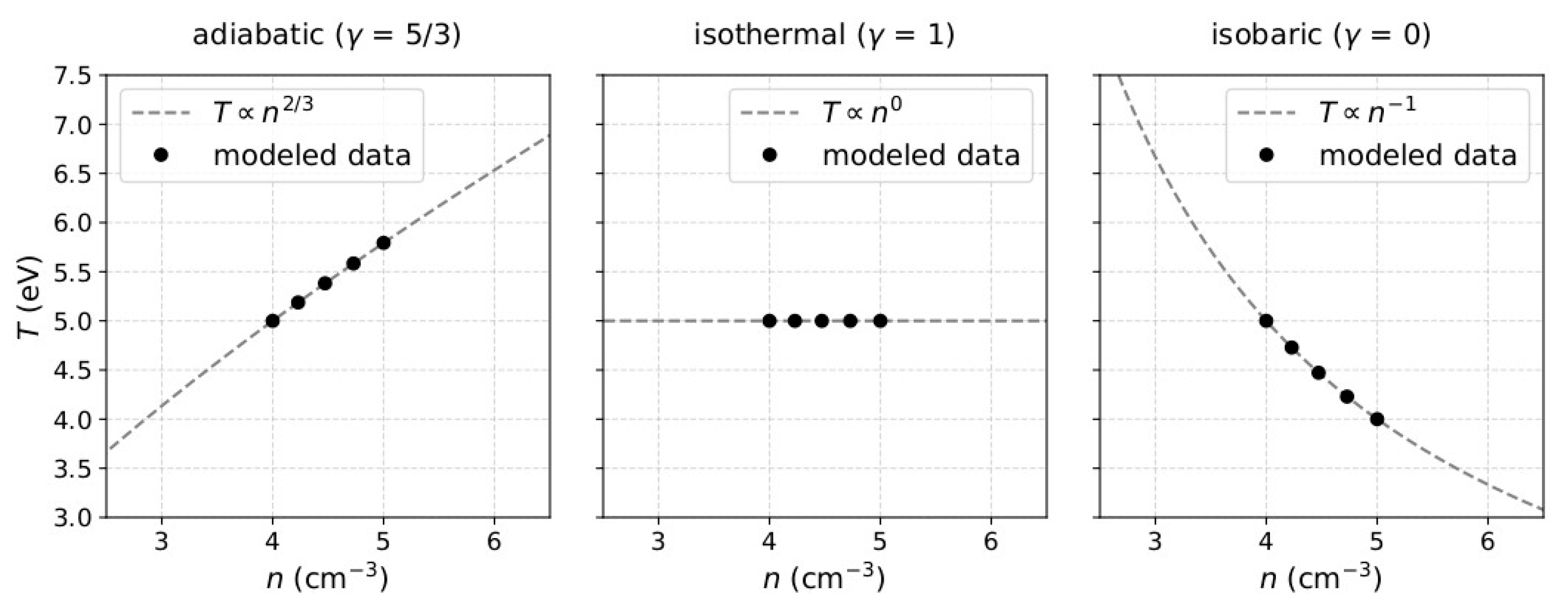
which we define for the minimum value of density nmin and a corresponding reference temperature value T0 within the interval. Note that, for γ > 1, T0 is the minimum temperature Tmin, while for γ < 1, is the maximum temperature Tmax within the time interval. The number of data-points, nmin, nmax, Tmin, and Tmax within each modeled interval should be adjusted for specific applications, as we do in Section 4 and Section 5. However, for the general model demonstration here, we consider typical values of solar wind plasma protons, within short time intervals (up to eight minutes) covered in five consecutive observations of ~1 to 1.5-min resolution (e.g., [14,16,24,25,26]). The selection of short time intervals in the referred studies, aims to reduce the possibility of streamline mixing within the observations. In Figure 1, we show examples of the modeled density and temperature for three characteristic values of γ.
2.2. Density and Temperature Uncertainties
The uncertainties (one-sigma error) of the observed density and temperature are
respectively. The subscript f denotes the uncertainties of the parameters due to natural plasma fluctuations (e.g., shocks, turbulence) in time scales shorter than the time resolution of the measurements. Typical plasma instruments complete a measurement by sampling the plasma in a finite time, and changes in the plasma parameters within the sampling time are not resolved [34]. These uncertainties are dependent on the polytropic relation. The subscript m denotes the measurement uncertainties of the quantities due to limited counting statistics and instrument capabilities (e.g., limited angular and energy resolution). Typical solar wind proton measurement uncertainties are within a few percent (e.g., [35]). Moreover, for high time resolution measurements, we can assume that and , therefore,
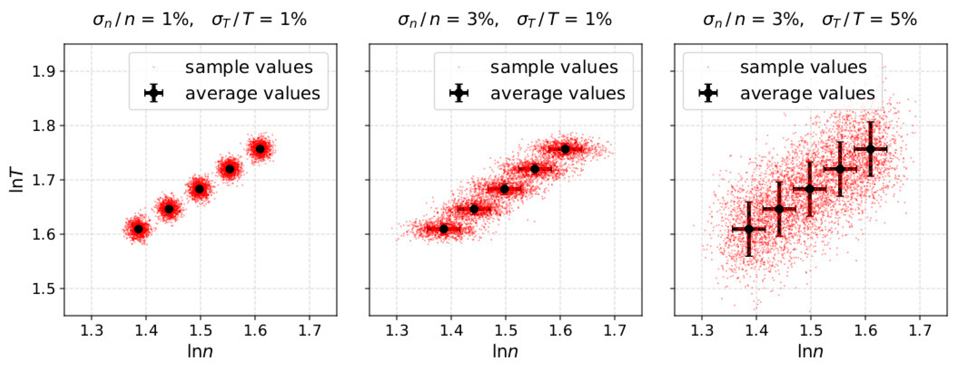
This work quantifies the misestimation of γ due to σn and σT. For the purpose of our study, we assign uncertainty in the modeled ni and Ti by modeling 1000 measurement samples of each data-point, assuming that the 1000 samples, follow a log-normal distribution (e.g., [35,36,37]) with standard deviation determined by the uncertainty level. We specifically model and with the index i denoting the data-point within the interval (ranging from 1 to 5) and j denoting the measurement sample (ranging from 1 to 1000). The 1000 and values of each ith data-point, are normally distributed, with mean values and following the polytropic model as described above, and non-dependent standard deviations and , respectively. In Figure 2 we show three examples of modeled samples with different uncertainty in the plasma density and temperature.
3. Analysis
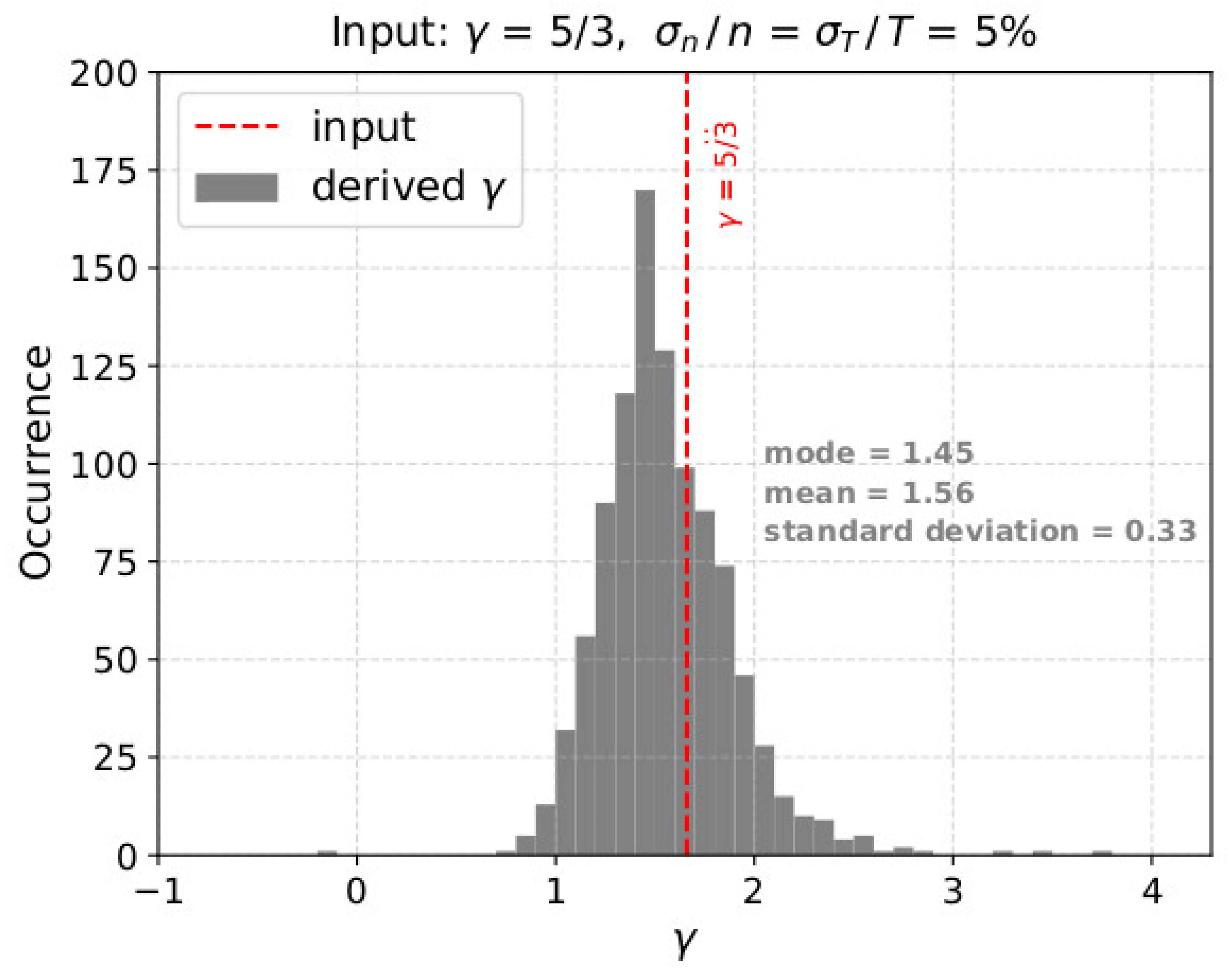
As described above, for each input polytropic index γ value and uncertainty level, we model 1000 interval samples. We then use a traditional chi-squared minimization method to fit the linear model of Equation (2) to the modeled lnT as a function of the modeled lnn, in each of the 1000 samples. Therefore, for each input, we derive 1000 values of γ using a fitting analysis which is used for actual space plasma applications. In Figure 3, we show the histogram of the 1000 polytropic index values as derived from the analysis of an adiabatic plasma model with density and temperature uncertainty σn/n = σT/T = 5%. As we introduce uncertainty in the plasma measurements, γ is derived within a finite range of values. In addition, the average and the most frequent values of the derived γ are different from the input value. The comparison between the input and the derived γ values, allows the quantification of the analysis accuracy as a function of the density and temperature uncertainties.
4. Results
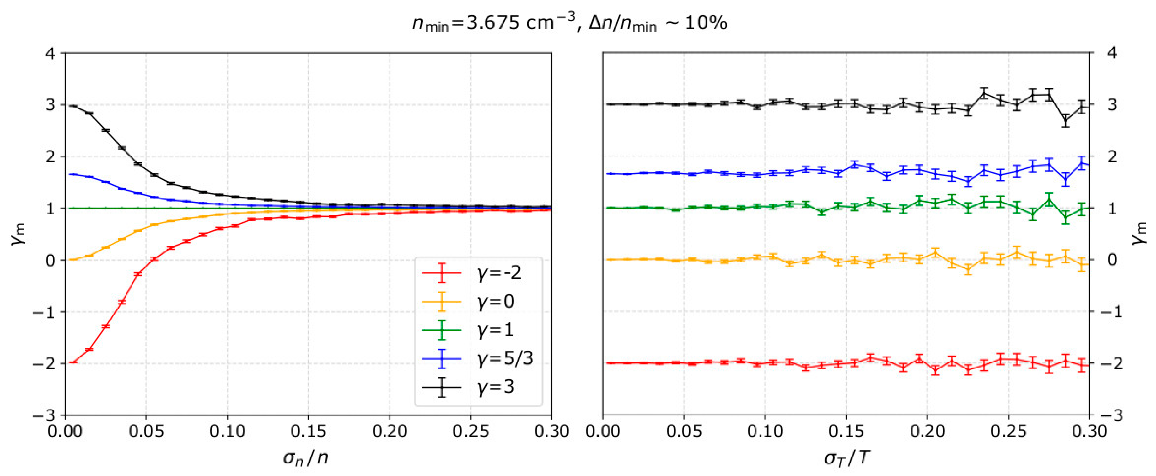
For each input γ, and specific uncertainty level, we calculate the mean γm and the standard error of the mean δγ as calculated for 1000 modeled samples. We then repeat for several uncertainty levels and for different input γ values. In the left panel of Figure 4, we show the calculated mean γm as a function of the uncertainty in the plasma density measurements and for no uncertainty in the temperature measurements, while the right panel shows the results as a function of the temperature measurement uncertainty and for no uncertainty in the density measurements. Both panels show the results for five different input γ values. For all the examples in Figure 4 we set nmin = 3.675 cm−3, Δn = nmax − nmin = 0.35 cm−3, and T0 = 3.275 eV, which are the most frequent values for solar wind plasma protons measured by Wind in 2002 (see Section 5).
Our results show that, with the standard linear fitting of lnT as a function of lnn, the polytropic index is misestimated due to uncertainties in the plasma density. As increases, the mean γm is shifted towards 1. For example, when analyzing plasma with polytropic index γ = 3 (black line in Figure 4), the standard fitting analysis will estimate γ < 1.5 as > 10% within the analyzed intervals. Additionally, for all the γ values we examine here, the plasma is misinterpreted as nearly-isothermal (γ~1) for > 15%.
The right panel of Figure 4 indicates that there is no systematic misestimation of the polytropic index as a function of the temperature uncertainties. On the other hand, the standard error of the mean polytropic index δγ, increases with , which means that the polytropic index is calculated within a broader range of values. For all the examples we examine here, the standard error δγ does not exceed a few percent of the mean value γm.
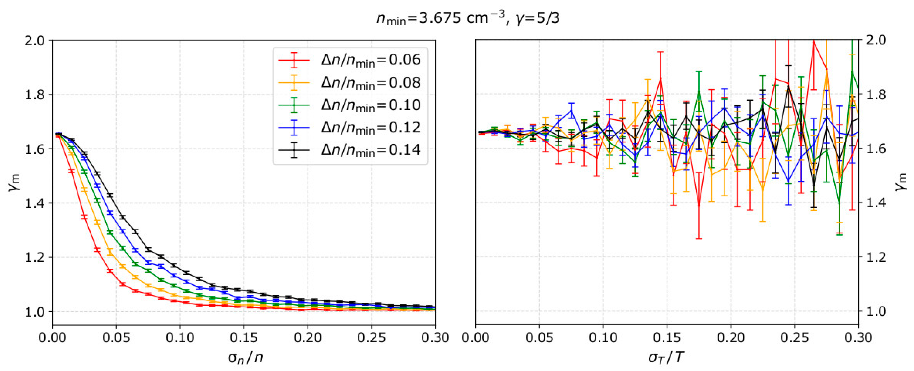
We further examine the dependence of the derived γm on and , for several Δn ranges within the analyzed subintervals. In Figure 5, we show our model results for adiabatic plasma and Δn/nmin values ranging from 0.06 to 0.14. The linear fitting is more accurate as Δn/nmin increases. In other words, for the same level of plasma uncertainties, the accuracy of the fit increases as the actual change of the plasma density within the interval increases. Additionally, for the range of plasma parameters we examine here, the uncertainty in the plasma temperature introduces noise in the derived γ.
5. Application to Solar Wind Protons
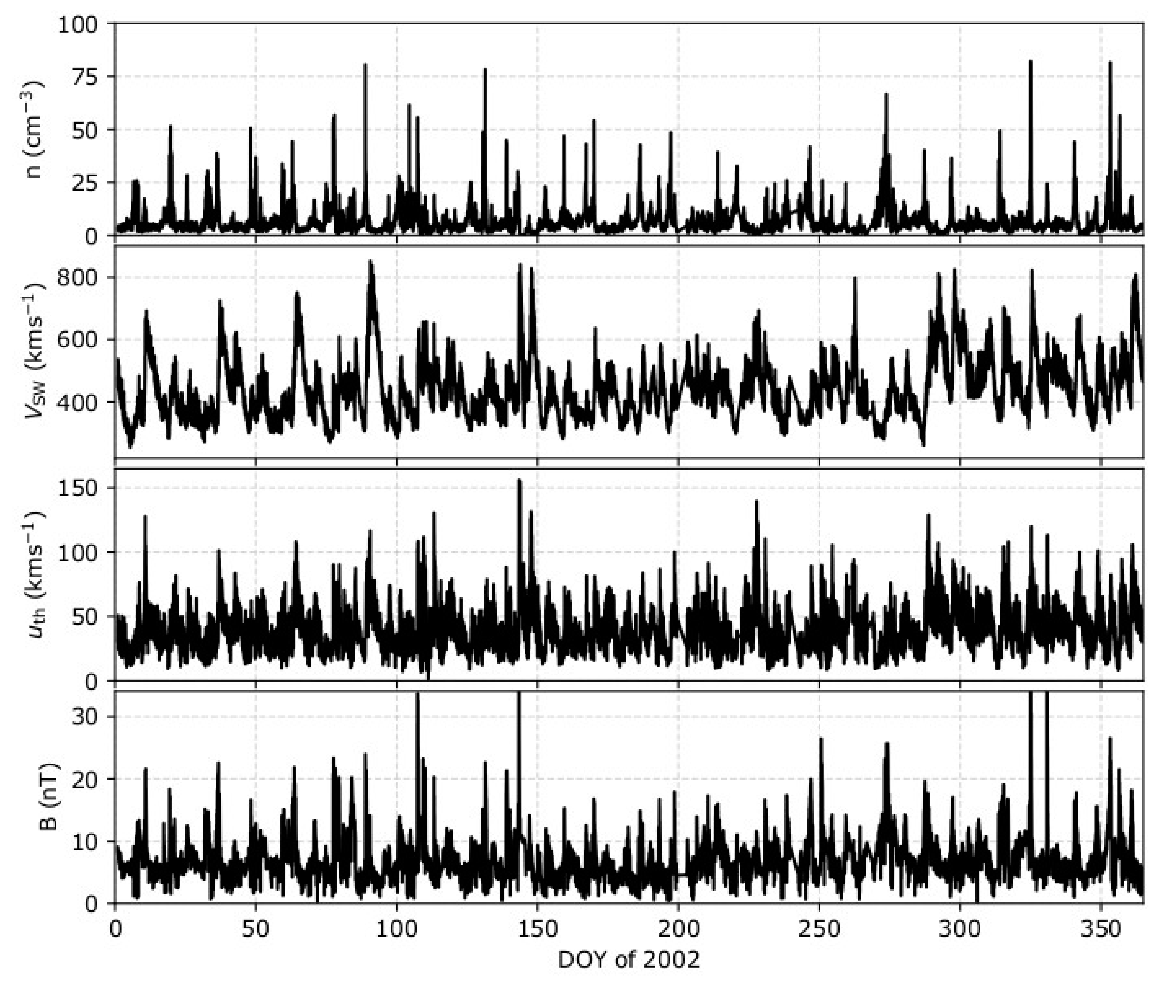
Our model predicts that uncertainties in the plasma measurements can lead to significant misestimation of the polytropic index. We now investigate and apply the model predictions to solar wind data. We analyze high-resolution (92 s) solar wind proton and magnetic field observations by Wind spacecraft. Wind’s Solar Wind Experiment (Wind/SWE, [38]) measures the reduced velocity distribution of solar wind protons, from which proton bulk parameters are derived by non-linear fitting of bi-Maxwellian distribution functions to the observations [39]. The non-linear fitting also provides the one-sigma error of the derived parameters. The solar wind magnetic field components, which we use to estimate the Bernoulli integral within selected intervals, are measured by Wind/MFI [40]. Here, we analyze the data obtained in 2002. The specific year does not have large data-gabs, and moreover, it has a significant amount of suitable intervals (~250,000) for a polytropic index analysis as a function of the parameter uncertainties. Figure 6 shows the time series of the plasma density n, bulk speed Vsw, thermal speed uth, and magnetic field B, as determined from non-linear fitting to the plasma observations, and the magnetic field magnitude, over the year 2002. (All datasets can be found in: https://cdaweb.gsfc.nasa.gov/index.html/).
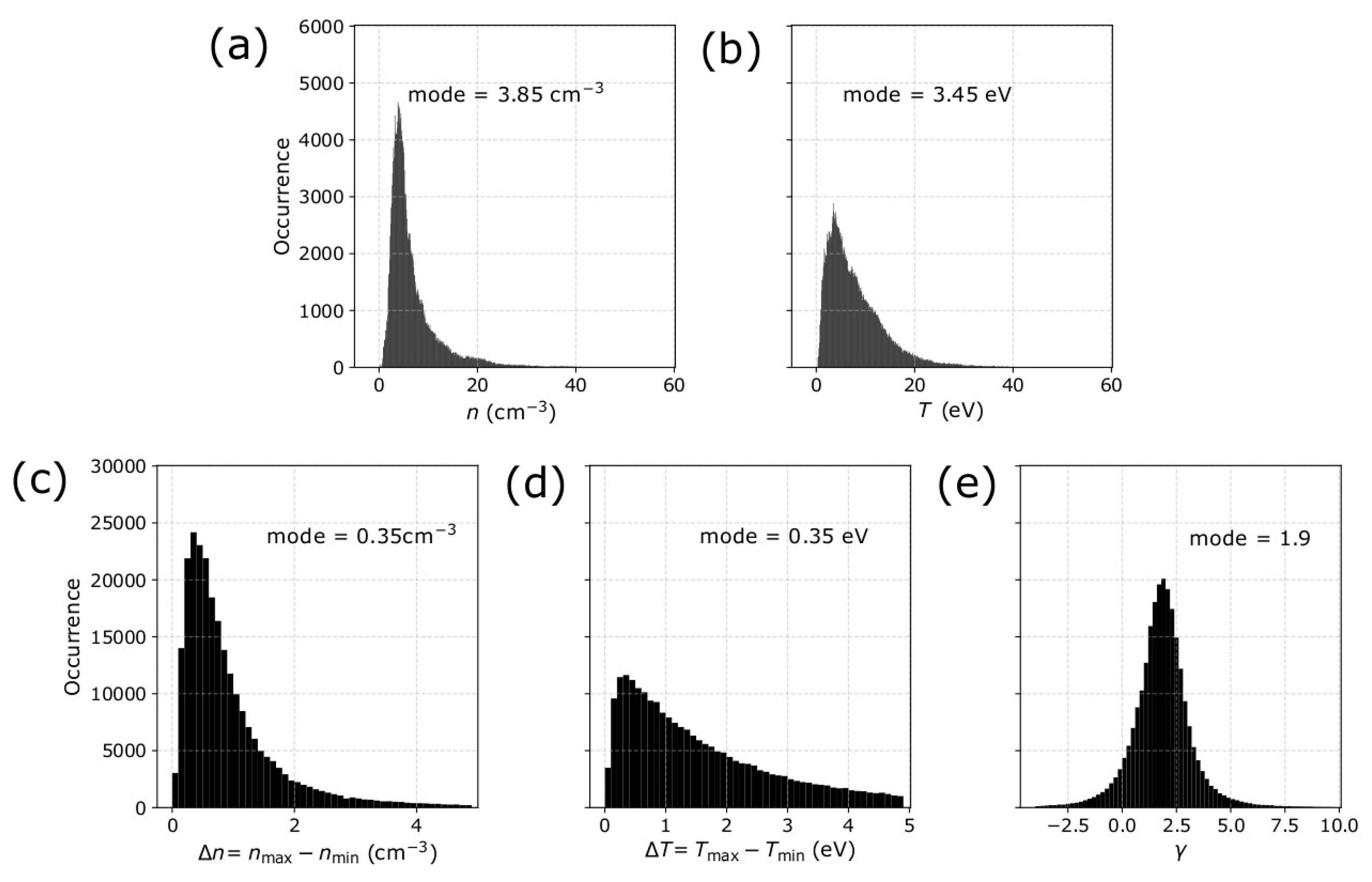
Following the analyses by references [3,14,16,18,20,24,26], we select intervals of five consecutive measurements (covering ~8 min of observations) that are characterized by a quasi-constant Bernoulli integral, and we derive γ by applying a linear fitting to lnT as a function of lnn. In Figure 7, we show the histogram of the average n, T, Δn, ΔT, and γ within the analyzed intervals in 2002. In each panel, we indicate the most frequent value (mode) of the corresponding parameters.
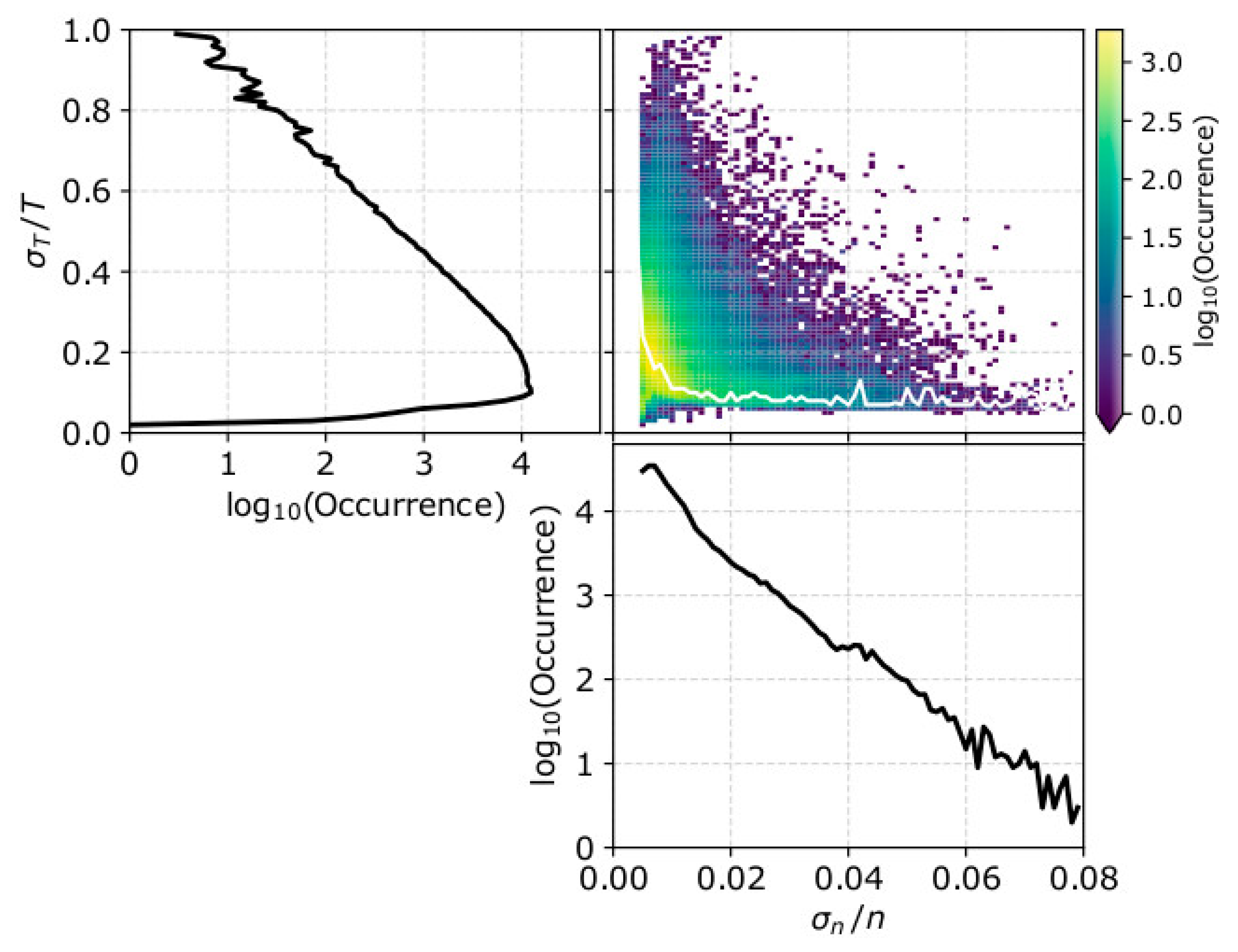
We also calculate the average (over the five consecutive measurements) sigma error and within each subinterval. Figure 8 shows the occurrences of , and their 2D histogram for the analyzed subintervals in 2002. The relative density error is recorded up to ~8% while the temperature relative error extends up to ~100%. We remind the reader that for a straight comparison with our model, we assume that the relative errors and are fair estimates of and , the standard deviations of lnn and lnT, respectively. The 2D histogram in the top right panel indicates that there is an anti-correlation between and . In order to compare the effects of one parameter uncertainty on the calculation of γ, we need to eliminate the effect of the uncertainty in the other parameter. Therefore, we select threshold values of < 1% and < 15%, chosen so that while we eliminate the effects of the corresponding parameter, we include a significant amount of data-points over a wide range of the examined parameters (see Figure 8).
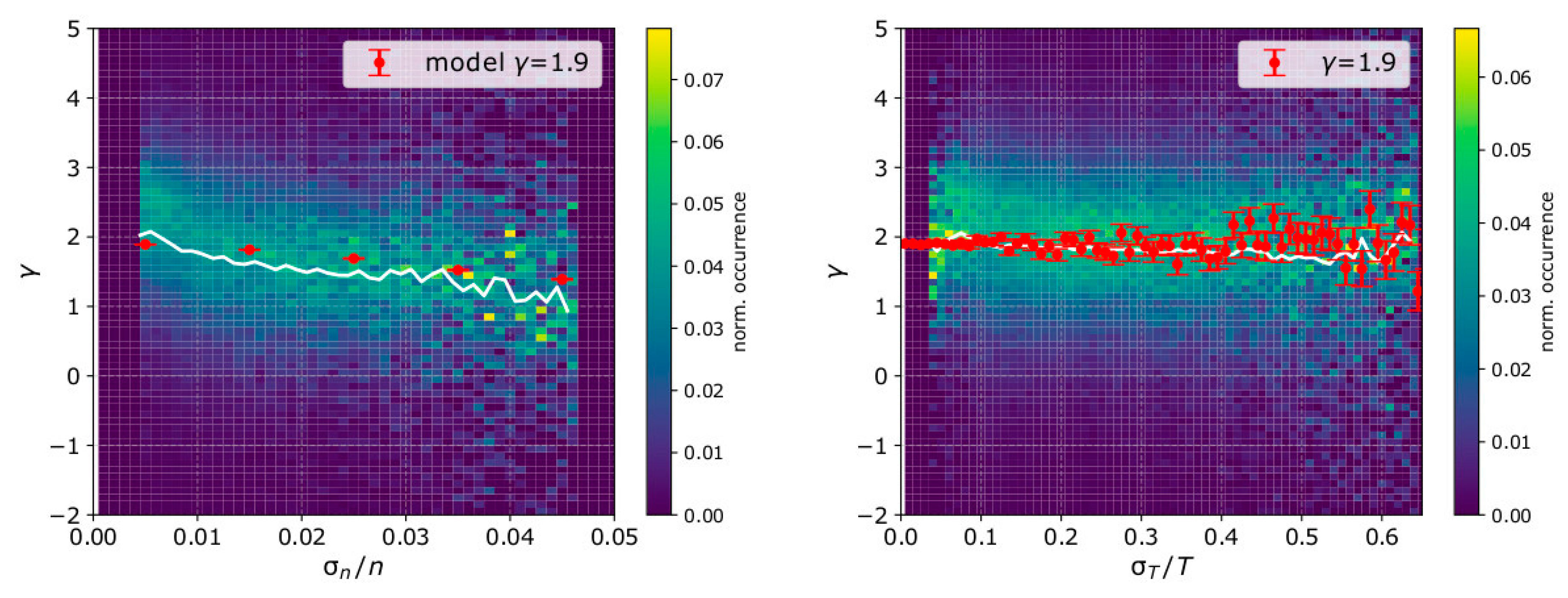
We further examine the calculated polytropic index as a function of the measurement uncertainties. The left panel of Figure 9 shows the 2D histogram of γ occurrence (normalized per column) as a function of , for < 15%, while the right panel shows the corresponding 2D histogram of γ as a function of , for < 1%. On the top of each histogram, we plot the predictions of our model for input parameters n, T, Δn, ΔT, and γ, set to the mode values of the corresponding parameters within the analyzed intervals over 2002 (mode values shown in Figure 7).
The data-analysis of the solar wind protons shows a clear dependence of the calculated γ as a function of . For low levels of density uncertainty, the average γ ~ 1.9, while it drops to γ ~ 1.5 as σn/n ~ 5%. Our model suggests that while the actual average γ ~1.9, it is possibly underestimated as the density measurement uncertainty increases. The uncertainty in the plasma temperature does not cause any systematic misestimation of γ, which is also compatible with our model predictions. Although our model considers one universal value for γ, the actual measurements possibly include plasma structures that expand under different conditions, which contributes to the spread of the calculated γ in Figure 9. However, we consider that our model values can represent the mean values of the measured γ, and we argue that the systematic behavior of γ as a function of the uncertainties could be an artifact related to the fitting method and not necessarily an actual difference in the plasma expansion conditions. We discuss our results further, in the next section.
6. Discussion
We show that the traditional calculation of the polytropic index from the linear fitting to lnT as a function of lnn data is sensitive to the accuracy with which the plasma parameters are measured. The uncertainties in the plasma density introduce random scattering of the fitted data-points along the x-direction of the Cartesian coordinate system we use for the fitting. As the scattering increases, the chi-squared value of the fitting is minimized for a linear model with slope closer to 0, introducing systematic error in the calculation of γ and occasionally, lead to artificial isothermal indices (γ ~ 1). On the other hand, uncertainties in the plasma temperature introduce random scattering of the data-points along the y-direction, leading to a larger statistical error in the calculation of γ. A relevant study by Livadiotis [41] investigates and discusses in detail the accuracy of the linear fitting method as a function of the reference frame. The magnitude of the propagated error (systematic and statistical) in γ is a function of the relative errors, and , and the corresponding parameter ranges Δn = nmax − nmin and ΔT = Tmax − Tmin in the examined intervals. We also expose this misestimation by analyzing actual solar wind proton data. Here, we discuss possible ways to filter the data and avoid erroneous calculations of γ.
6.1. Uncertainty Threasholds
One reasonable and straight forward approach that reduces the error in the calculated γ, is the data filtering, which excludes data-points with large measurement uncertainties. Although such an approach reduces the amount of analyzed data, it will improve the accuracy of the derived γ indices. Our study quantifies the linear fit accuracy as a function of the measurement uncertainties, the range of n within the intervals, and for several γ indices (e.g., Figure 4 and Figure 5). In conclusion, future polytropic index analyses that use the traditional fitting should follow our techniques to optimize the thresholds in their data-filtering according to the accuracy requirement in each application.
6.2. Correlation Coefficient Filter
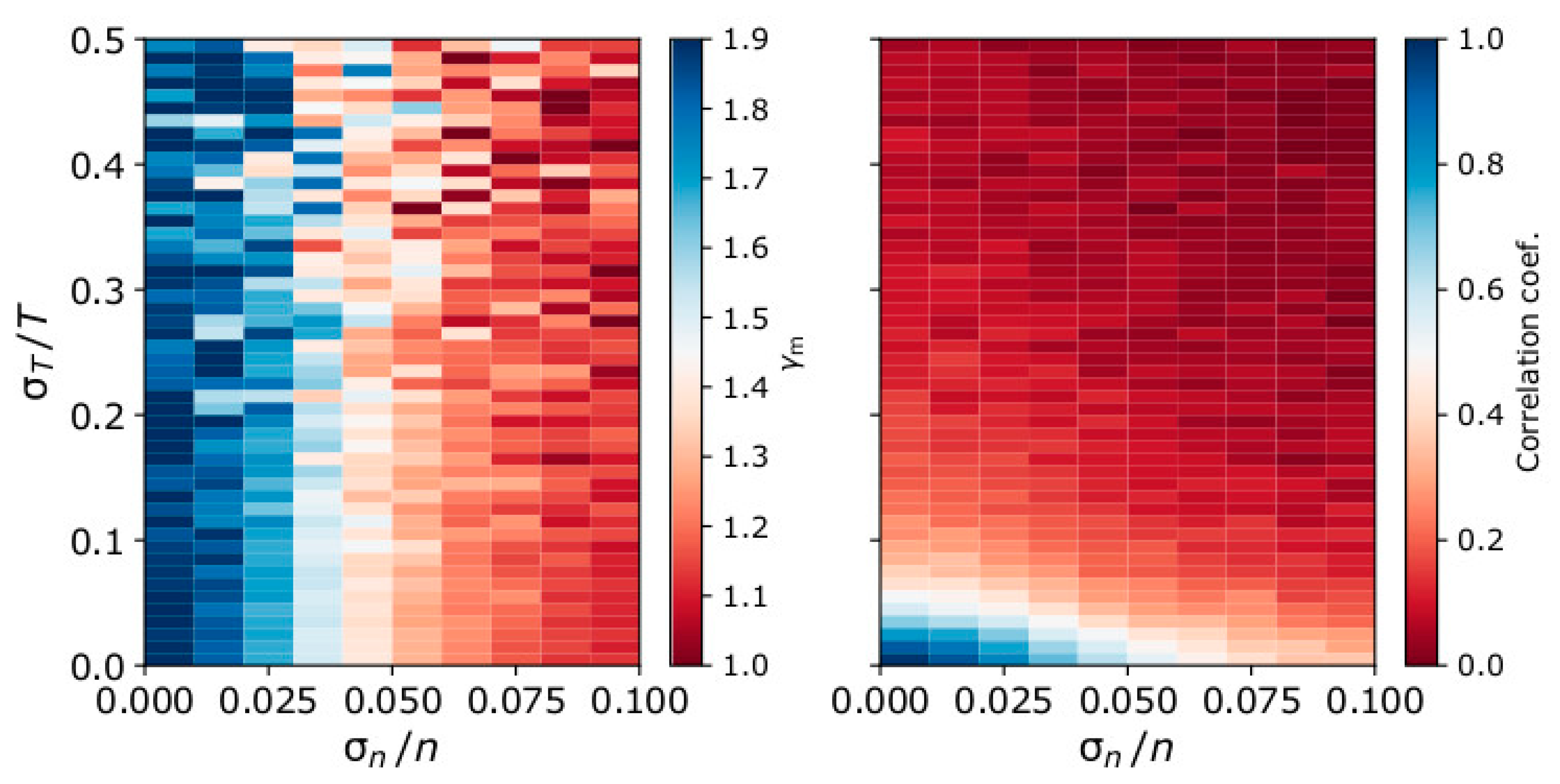
Large uncertainties in the plasma density and temperature reduce the absolute correlation coefficient value of the linear fits to the lnT–lnn data. In the left panel of Figure 10, we plot the 2D histogram of the mean γm as a function of and as predicted by our model for input γ = 1.9. In the right panel of Figure 10, we show the 2D histograms of the average correlation coefficient of the linear fittings to lnT–lnn. The average γm and the average correlation coefficients are calculated over 1000 modeled samples for each and combination. One approach to reducing the amount of erroneous data is to filter the results based on the correlation coefficient between lnT–lnn within the analyzed intervals. The selected correlation threshold should be optimized according to the desired accuracy. Nevertheless, such a filter excludes real isothermal cases from the analysis (e.g., [24]).
6.3. Proposed Approach Cased on the Special Polytropic Index V
According to the polytropic relation in Equation (1), the density as a function of temperature is
where the special polytropic index
Taking the logarithm of Equation (7):
and in data-analyses, the index ν can be calculated by applying a linear model to lnn as a function of lnT. The function in Equation (9) is the inverse of the function in Equation (2), and the derived by a fitting index νinv, similarly to γ, is also affected by the plasma measurement uncertainties.
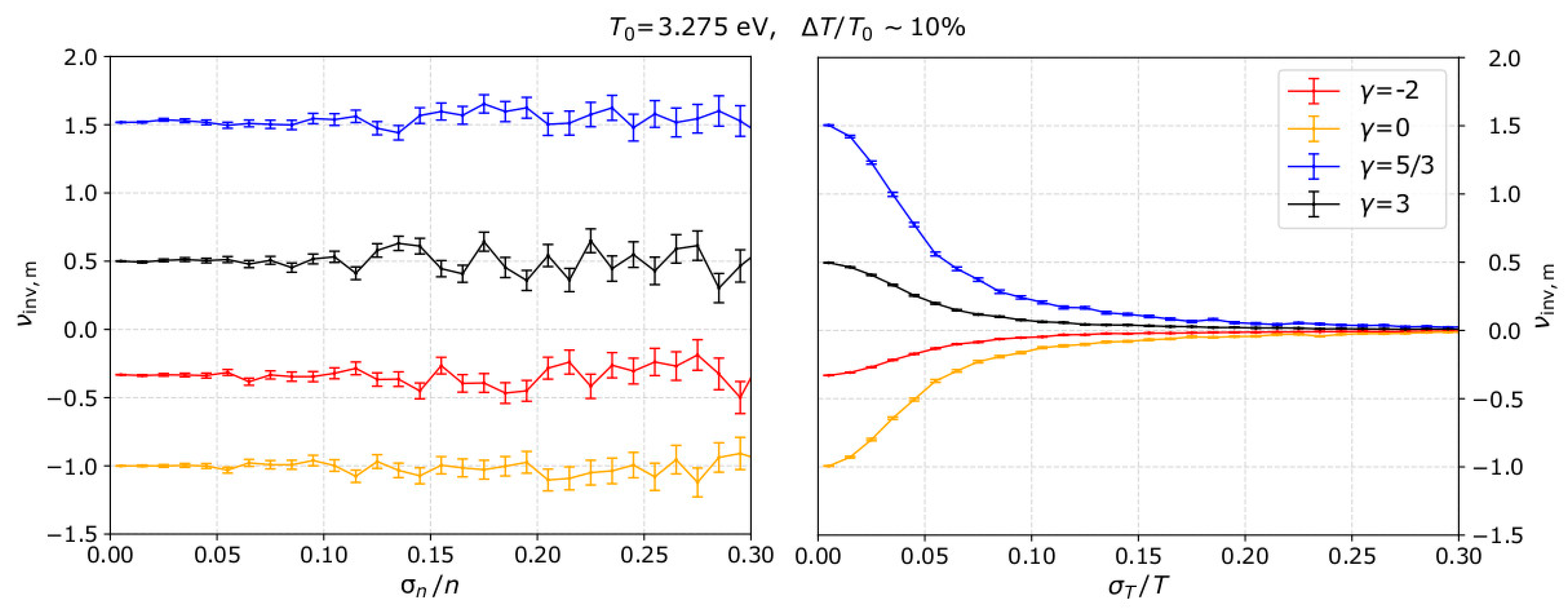
In order to demonstrate and examine the dependence of νinv on the measurement uncertainties, we run model plasma measurements in a similar manner as described in Section 2, and we derive νinv as the slope of the line fitted to lnn as a function of lnT. In the left panel of Figure 11, we plot the average estimated νinv,m as a function of for = 0, while in the right panel we show νinv,m as a function of for = 0. In such a chi-square minimization fitting, the uncertainties in the plasma density propagate a statistical error in the calculation of νinv, while uncertainties in the plasma temperature introduce a systematical error by shifting the estimated νinv towards zero.
The accuracy of the estimated γ and νinv, is affected by and . However, (γ-1) and νinv are the slopes of two inverse functions and are related by the identity in Equation (8) which we rewrite as
Equation (10) implies that we need to validate intervals for which
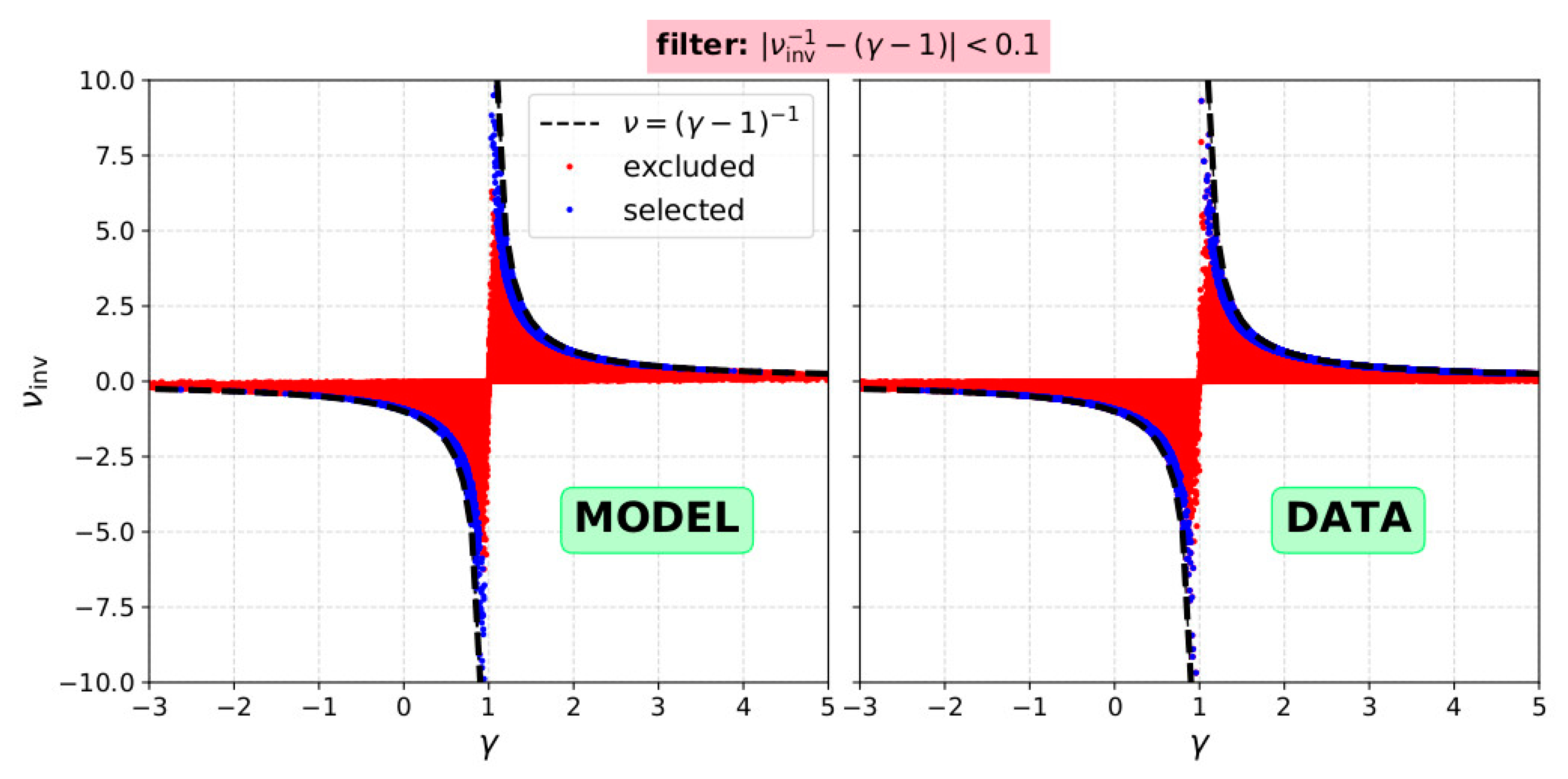
where α is a threshold value to be determined according to the desired accuracy of the results. In Figure 12 we plot the calculated ν as a function of the calculated γ for ~250,000 samples (comparable to the amount of analyzed intervals in 2002) with input γ = 1.9 and = = 8%. The input uncertainty in the parameters considers the highest levels in density uncertainty measured in 2002 (see Figure 8). We demonstrate which data-points will be excluded as we apply a filter according to Equation (11) for a threshold value α = 0.1. In the right panel of Figure 12, we show in the same format, the indices as calculated form Wind data during 2002. In both plots, the dashed line indicates the ν ≡ (γ − 1)−1. The distribution of the data points in the model and the distribution of the actual data are virtually the same. We emphasize on the fact that as expected, for ν > 0, all the data-points reside on the left of the dashed line, and for ν < 0, all the data-points reside on the right of the dashed line. This reflects the fact that the uncertainties in n shift γ towards 1, while uncertainties in T shift νinv towards 0.
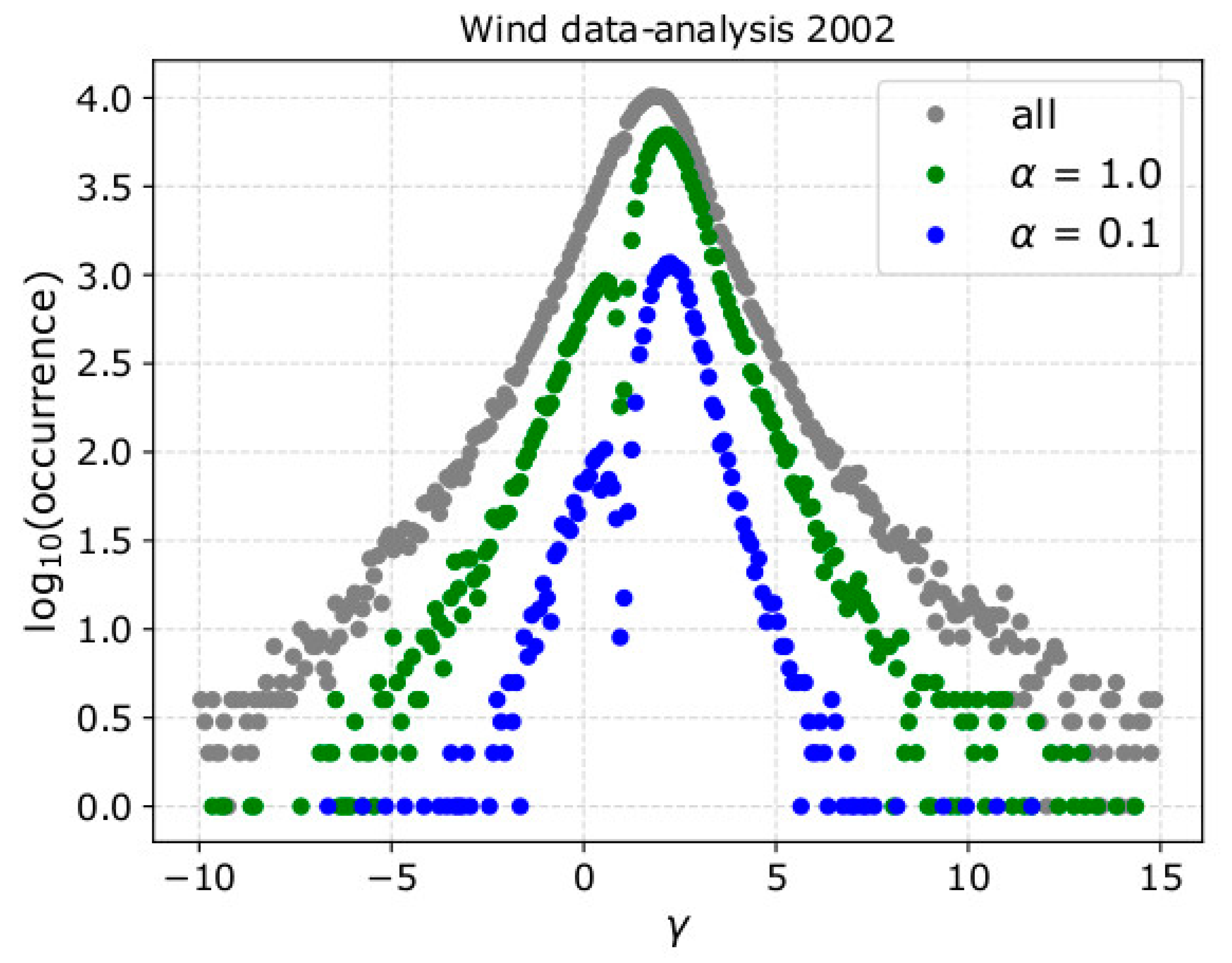
In Figure 13, we show the histogram of γ as derived by the data-analysis of the Wind observations over 2002, before (grey) and after the filter application with (green) α = 1, and (blue) α = 0.1. As expected, the filter selects a percentage of the available data-points. The filtered γ is recorded over a shorter range of values. The amount of filtered data-points decreases with decreasing α, which sets the accuracy requirements. There is a sharp dip in the histogram of the filtered values for γ = 1, which corresponds to isothermal plasma. For these intervals, the linear fitting cannot determine a value of the polytropic index ν, which is approaching ∞, thus, are excluded from the analysis. Finally, we note that here we apply the proposed filter in subintervals of fixed length (~8 min) in order to automatically validate the identity in Equation (8) with fixed accuracy. The plasma within the rejected subintervals is possibly measured with high uncertainty, and the accuracy requirement set by the filter is not met. Moreover, the plasma in those subintervals may not correspond in uniform plasma with a single polytropic index. More sophisticated methods can investigate the polytropic relation in different timescales and by applying more complicated polytropic models [3,4].
7. Summary and Conclusions
In this paper, we examined the misestimation of the space plasma polytropic index using spacecraft measurements and a linear fit to the measured lnT as a function of lnn. We quantify the expected error as a function of the plasma density and temperature measurement uncertainties, considering several characteristic polytropic behaviors. We further analyzed Wind observations in order to derive the polytropic index of the solar wind protons over 2002 and examined its behavior as a function of the measurement uncertainties.
We concluded that:
- Density measurement uncertainties shift the estimated polytropic index towards 1. For density uncertainties comparable with the range of density variation during the analyzed intervals, the linear fit cannot resolve any real expansion or compression of the plasma and returns artificial isothermal relation;
- Temperature measurement uncertainties introduce statistical error in the calculation of the polytropic index;
- The correlation coefficient drops drastically as the plasma measurement uncertainties increase, therefore, it can be used as a potential criterion to filter erroneous data. Nevertheless, such a criterion will also exclude real, nearly isothermal cases;
- When using standard least square fitting, we can filter erroneous data by calculating the special polytropic index ν and exclude intervals for which ν differs significantly from its definition value . We demonstrated our suggested approach using the solar wind proton measurements by Wind in 2002.
Therefore, future analyses on the polytropic index determination must be cautious of the possible misinterpretations due to measurement uncertainties and apply appropriate filters to the data, as suggested here. Finally, we highlight the importance of the accurate determination of γ since it is a crucial parameter in understanding the physical mechanisms in plasmas and it is related to the kappa index that labels and governs the velocity distribution functions of the plasma particles [14,15,16]. Future studies can address the polytropic behavior of different solar wind structures, in different time scales, and by adjusting several data-selection criteria.
Author Contributions
Conceptualization, G.N. and G.L.; methodology, G.N. and G.L.; software, G.N.; validation, G.N., G.L. and R.T.W.; formal analysis, G.N.; investigation, G.N., G.L. and R.T.W.; resources, G.N., G.L. and R.T.W.; data curation, G.N.; writing—original draft preparation, G.N.; writing—review and editing, G.N., G.L. and R.T.W.; visualization, G.N.; project administration, R.T.W.; funding acquisition, R.T.W.
Acknowledgments
G.N. and R.T.W. are supported by the STFC Consolidated Grant to UCL/MSSL, ST/S000240/1. G.L. is supported by a Nasa’s projects NNX17AB74G and 80NSSC18K0520.
Conflicts of Interest
The authors declare no conflict of interest.
References
- Parker, E.N. Interplanetary Dynamical Processes; Wiley-Interscience: Hoboken, NJ, USA, 1963. [Google Scholar]
- Chandrasekhar, S. An Introduction to the Study of Stellar Structure; Dover Publications: New York, NY, USA, 1967. [Google Scholar]
- Livadiotis, G. Superposition of polytropic in the inner heliosheath. Astrophys. J. Suppl. Ser. 2016, 223, 1–13. [Google Scholar] [CrossRef]
- Nicolaou, G.; Livadiotis, G. Modeling the plasma flow in the inner heliosheath with a spatially varying compression ratio. Astrophys. J. 2017, 838, 7. [Google Scholar] [CrossRef]
- Totten, T.L.; Freeman, J.W.; Arya, S. An empirical determination of the polytropic index for the free-streaming solar wind using Helios 1 data. J. Geophys. Res. 1995, 100, 13–17. [Google Scholar] [CrossRef]
- Osherovich, V.A.; Fainberg, J.; Stone, R.G. Multi-tube model for interplanetary magnetic clouds. Geophys. Res. Lett. 1999, 26, 401–404. [Google Scholar] [CrossRef]
- Gosling, J.T. On the determination of electron polytrope indices within coronal mass ejections in the solar wind. J. Geophys. Res. 1999, 104, 19851–19857. [Google Scholar] [CrossRef] [Green Version]
- Spreiter, J.R.; Stahara, S.S. Gasdynamic and magnetohydrodynamic modeling of the magnetosheath: A tutorial. Adv. Space Res. 1994, 14, 5–19. [Google Scholar] [CrossRef]
- Parker, E.N. The stellar-wind regions. Astrophys. J. 1961, 134, 20–26. [Google Scholar] [CrossRef]
- Livadiotis, G. Shock strength in space and astrophysical plasmas. Astrophys. J. 2015, 809, 111. [Google Scholar] [CrossRef]
- Scherer, K.; Fichtner, H.; Fahr, H.J.; Röken, C.; Kleimann, J. Generalized multi-polytropic Rankine-Hugoniot relations and the entropy conditions. Astrophys. J. 2016, 833, 38–48. [Google Scholar] [CrossRef]
- Akiyama, K.; Alberdi, A.; Alef, W.; Asada, K.; Azulay, R.; Baczko, A.K.; Ball, B.; Baloković, M.; Barrett, J. First M87 Event Horizon Telescope Results. V. Physical Origin of the Asymmetric Ring. Astrophys. J. Lett. 2019, 875, L5. [Google Scholar]
- Bruno, R.; Carbone, V. The solar wind as a turbulence laboratory. Living Rev. Sol. Phys. 2013, 4, 1–187. [Google Scholar] [CrossRef]
- Livadiotis, G. Using kappa distributions to identify the potential energy. J. Geophys. Res. 2018, 123, 1050–1060. [Google Scholar] [CrossRef]
- Livadiotis, G. On the polytropic behavior in space and astrophysical plasma. Astrophys. J. 2019, 874, 10–18. [Google Scholar] [CrossRef]
- Nicolaou, G.; Livadiotis, G. Long term correlations of polytropic indices with kappa distributions in solar wind plasma near 1 au. Astrophys. J. 2019, 884, 52. [Google Scholar] [CrossRef]
- Newbury, J.A.; Russel, C.T.; Lindsay, G.M. Solar wind polytropic index in the vicinity of stream interactions. Geophys. Res. Lett. 1997, 24, 1431–1434. [Google Scholar] [CrossRef]
- Kartalev, M.; Dryer, M.; Grigorov, K.; Stoimenova, E. Solar wind polytropic index estimates based on single spacecraft plasma and interplanetary field measurements. J. Geophys. Res. 2006, 111, A10107. [Google Scholar] [CrossRef]
- Osherovich, V.A.; Farrugia, L.F.; Burlaga, L.F.; Lepping, R.P.; Fainberg, J.; Stone, R.G. Polytropic relation in interplanetary clouds. J. Geophys. Res. 1993, 98, 15331–15342. [Google Scholar] [CrossRef]
- Pang, X.; Cao, J.; Liu, W.; Ma, Y.; Lu, H.; Yang, J.; Li, L.; Liu, X.; Wang, J.; Wang, T.; et al. Polytropic index of central plasma sheet ions based on MHD Bernoulli integral. J. Geophys. Res. 2015, 120, 4736–4747. [Google Scholar] [CrossRef]
- Park, J.-S.; Shue, J.-H.; Nariyuki, Y.; Kartalev, M. Dependence of thermodynamic processes on upstream interplanetary magnetic field conditions for magnetosheath ions. J. Geophys. Res. 2019, 124, 1866–1882. [Google Scholar] [CrossRef]
- Roussev, I.I.; Gombosi, T.I.; Sokolov, I.V.; Velli, M.; Manchester, W.; DeZeeuw, D.L.; Liewer, P.; Tόth, G.; Luhmann, J. A three-dimensional model of the solar wind incorporating solar magnetogram observations. Astrophys. J. 2003, 595, 57–61. [Google Scholar] [CrossRef]
- Meister, C.-V.; Maurer, C.; Hoffmann, D.H.H. Effective polytropic indices of anisotropic magnetosheath plasmas with magnetoacoustic waves. Contrib. Plasma Phys. 2011, 51, 639–649. [Google Scholar] [CrossRef]
- Nicolaou, G.; Livadiotis, G.; Moussas, X. Long-term variability of the polytropic index of solar wind protons at 1 AU. Sol. Phys. 2014, 289, 1371–1378. [Google Scholar] [CrossRef]
- Livadiotis, G.; Desai, M.I. Plasma-field coupling at small length scales in solar wind near 1 au. Astrophys. J. 2016, 829, 88. [Google Scholar] [CrossRef]
- Livadiotis, G. Long-term independence of solar wind polytropic index on plasma flow speed. Entropy 2018, 20, 799. [Google Scholar] [CrossRef]
- Schwenn, R. Large-Scale Structure of the Interplanetary Medium, in Physics of the Inner Heliosphere; Springer: Berlin/Heidelberg, Germany; New York, NY, USA, 1990; Volume 1. [Google Scholar]
- Dialynas, K.; Roussos, E.; Regoli, L.; Paranicas, C.P.; Krimigis, S.M.; Kane, M.; Mitchell, D.G.; Hamilton, D.C.; Krupp, N.; Carbary, J.F. Energetic ion moments and polytropic index in Saturn’s magnetosphere using Cassini/MIMI measurements: A simple model based on κ-distribution functions. J. Geophys. Res. 2018, 123, 8066–8086. [Google Scholar] [CrossRef]
- Arridge, C.S.; McAndrews, H.J.; Jackman, C.M.; Forsyth, C.; Walsh, A.P.; Sittler, E.C.; Gilbertab, L.K.; Lewisab, G.R.; Russellf, C.T.; Coates, A.J.; et al. Plasma electrons in Saturn’s magnetotail: Structure, distribution and energisation. Planet. Space Sci. 2009, 57, 2032–2047. [Google Scholar] [CrossRef]
- Nicolaou, G.; McComas, D.J.; Bagenal, F.; Elliott, H.A. Properties of plasma ions in the distant Jovian magnetosheath using Solar Wind Around Pluto data on New Horizons. J. Geophys. Res. 2014, 119, 3463–3479. [Google Scholar] [CrossRef]
- Livadiotis, G.; McComas, D.J.; Schwadron, N.A.; Funsten, H.O.; Fuselier, S.A. Pressure of the proton plasma in the inner heliosheath. Astrophys. J. 2013, 762, 134. [Google Scholar] [CrossRef]
- Livadiotis, G.; McComas, D.J. Non-equilibrium thermodynamic processes: Space plasmas and the inner heliosheath. Astrophys. J. 2012, 749, 11. [Google Scholar] [CrossRef]
- Livadiotis, G.; McComas, D.J. Fitting method based on correlation maximization: Applications in Astrophysics. J. Geophys. Res 2013, 118, 2863–2875. [Google Scholar] [CrossRef]
- Nicolaou, G.; Verscharen, D.; Wicks, R.T.; Owen, C.J. The Impact of Turbulent Solar Wind Fluctuations on Solar Orbiter Plasma Proton Measurements. Astrophys. J. 2019, in press. [Google Scholar]
- Kasper, J.C.; Lazarus, A.J.; Steinberg, J.T.; Ogilvie, K.W.; Szabo, A. Physics-based tests to identify the accuracy of solar wind ion measurements: A case study with the Wind Faraday Cups. J. Geophys. Res. 2006, 111, A03105. [Google Scholar] [CrossRef]
- Veselovsky, I.S.; Dmitriev, A.V.; Suvorova, A.V. Algebra and statistics of the solar wind. Cosmic Res. 2010, 48, 113. [Google Scholar] [CrossRef]
- Venzmer, M.S.; Bothmer, V. Solar-wind predictions for the Parker Solar Probe orbit: Near-Sun extrapolations derived from an empirical solar-wind model based on Helios and OMNI observations. Astron. Astrophys. 2018, 611, A36. [Google Scholar] [CrossRef]
- Ogilvie, K.W.; Chornay, D.J.; Fritzenreiter, R.J.; Hunsaker, F.; Keller, J.; Miller, G.; Scudder, J.D.; Sittler, E.C.; Torbert, R.B.; Bodet, D.; et al. SWE, a comprehensive plasma instrument for the WIND spacecraft. Space Sci. Rev. 1995, 71, 55–77. [Google Scholar] [CrossRef]
- Kasper, J. Solar Wind Plasma: Kinetic Properties and Micro-Instabilities. Ph.D. Thesis, Massachusetts Institute of Technology, Cambridge, MA, USA, 2003. [Google Scholar]
- Lepping, R.P.; Acũna, M.H.; Burlaga, L.F.; Farrel, W.M.; Slavin, J.A.; Schatten, K.H.; Mariani, F.; Ness, N.F.; Neubauer, F.M.; Whang, Y.C.; et al. The WIND magnetic field investigation. Space Sci. Rev. 1995, 71, 207–229. [Google Scholar] [CrossRef]
- Livadiotis, G. Linear Regression with Optimal Rotation. Stats 2019, 2, 416–425. [Google Scholar] [CrossRef] [Green Version]
Figure 1.
Model of plasma temperature T as a function of the modeled plasma density n for (left) adiabatic plasma with γ = 5/3, (middle) isothermal plasma with γ = 1 and (right) for isobaric plasma with γ = 0. In each panel, we plot (grey dashed). For all the examples here, the plasma density ranges between nmin = 4 cm−3 and nmax = 5 cm−3 and T0 = 5 eV.

Figure 2.
Modeled samples of lnT as a function of lnn, for adiabatic plasma and (left) = = 1%, (middle) = 3%, = 1% and (right) = 3%, = 5%. In each plot, the black data-points correspond to the modeled plasma parameters while the red dots correspond to the measurement samples. We model 1000 measurement samples, considering a log-normal distribution around the plasma parameters (black dots) and standard deviation as indicated by the error bar.

Figure 3.
Histogram of the derived γ over 1000 samples, considering adiabatic plasma, and uncertainties = = 5%. Although the modeled plasma has γ = 5/3, the distribution of the derived values is slightly asymmetric with the most frequent value 1.45 and mean γm ~1.56. The standard deviation of the distribution is σγ ~0.33. The plasma uncertainty in the plasma parameters introduces a systematical (different mean and mode) and statistical (σγ > 0) error in the calculation of γ.

Figure 4.
The average γm as a function of (left) density and (right) temperature measurement uncertainty. The average γm and its standard error δγ are calculated over 1000 samples of n-T measurements. Lines with different colors represent different input γ values. For the specific examples, we set nmin = 3.675 cm−3, Δn = nmax − nmin = 0.35 cm−3, and T0 = 3.275 eV, which correspond to typical values of solar wind protons as observed by Wind in 2002.

Figure 5.
The derived polytropic index averages (over 1000 samples) as a function of (left) density and (right) temperature measurement uncertainty, for several Δn ranges. For all the examples shown here, we consider an adiabatic plasma (input γ = 5/3).
Figure 5.
The derived polytropic index averages (over 1000 samples) as a function of (left) density and (right) temperature measurement uncertainty, for several Δn ranges. For all the examples shown here, we consider an adiabatic plasma (input γ = 5/3).

Figure 6.
Wind high-resolution measurements of (from top to bottom) density, bulk speed, thermal speed, and magnetic field strength, during 2002.
Figure 6.
Wind high-resolution measurements of (from top to bottom) density, bulk speed, thermal speed, and magnetic field strength, during 2002.

Figure 7.
Histogram of the average solar wind protons parameters within the selected subintervals in 2002, which we analyze to derive the polytropic index, (a) the average density n and (b) average temperature T, (c) density range Δn, (d) temperature range ΔT and (e) the derived polytropic index γ. In each panel, we note the most frequent value (mode) of each parameter, which we use as input to our model to predict the misestimation of γ as a function of the measurement uncertainties.

Figure 8.
Occurrence of (upper left) the average , (lower) the average and (upper right) the 2D histogram of and of the Wind observations in 2002. The white line indicates the mode of in each bin.
Figure 8.
Occurrence of (upper left) the average , (lower) the average and (upper right) the 2D histogram of and of the Wind observations in 2002. The white line indicates the mode of in each bin.

Figure 9.
Normalized histograms of (left) γ as a function of , for < 15% and (right) γ as a function of , for < 1%. The white line is the mean value of the histogram in each column. We display only the range of uncertainties for which we have more than 100 data points. On each panel, we show the predictions of our model (red) for plasma parameters corresponding to the mode values of each parameter for the analyzed intervals (see also Figure 7).

Figure 10.
The 2D histogram of (left) mean calculated polytropic index γm and (right) the average Pearson correlation coefficient of lnT and lnn as a function of and for modeled plasma with γ = 1.9, nmin = 3.675 cm−3, Δn = nmax − nmin = 0.35 cm−3, and T0 = 3.275 eV. The average polytropic indices and correlation coefficients are calculated for 1000 modeled measurement samples per each combination of − .

Figure 11.
(Left) average νinv,m as a function of for = 0 and (right) as a function of for = 0 and for several γ. The average νinv,m is calculated over 1000 samples for each uncertainty setting in our model. For the specific examples we consider T0 = 3.275 eV and ~ 10%.
Figure 11.
(Left) average νinv,m as a function of for = 0 and (right) as a function of for = 0 and for several γ. The average νinv,m is calculated over 1000 samples for each uncertainty setting in our model. For the specific examples we consider T0 = 3.275 eV and ~ 10%.

Figure 12.
(Left) the calculated ν as a function of the calculated γ for 250,000 samples with input γ = 1.9, = = 8%, and (right) the same plot for the analyzed intervals from Wind measurements during 2002. In both plots, the blue data-points satisfy the criterion | 1/νinv – (γ-1)| < 0.1, while the red-data points do not, as they lie further from the expected ν ≡ (γ − 1)−1 (dashed).

Figure 13.
Histograms of γ as derived by the analysis of Wind observation over 2002, before (grey) and after the filter application with (green) α = 1, and (blue) α = 0.1. The filtered γ values are recorded within a shorter range, and the corresponding histogram has a sharp dip at γ = 1 for which the linear fitting cannot derive an accurate ν index.

© 2019 by the authors. Licensee MDPI, Basel, Switzerland. This article is an open access article distributed under the terms and conditions of the Creative Commons Attribution (CC BY) license (http://creativecommons.org/licenses/by/4.0/).
Share and Cite
MDPI and ACS Style
Nicolaou, G.; Livadiotis, G.; Wicks, R.T. On the Calculation of the Effective Polytropic Index in Space Plasmas. Entropy 2019, 21, 997. https://0-doi-org.brum.beds.ac.uk/10.3390/e21100997
AMA Style
Nicolaou G, Livadiotis G, Wicks RT. On the Calculation of the Effective Polytropic Index in Space Plasmas. Entropy. 2019; 21(10):997. https://0-doi-org.brum.beds.ac.uk/10.3390/e21100997
Chicago/Turabian StyleNicolaou, Georgios, George Livadiotis, and Robert T. Wicks. 2019. "On the Calculation of the Effective Polytropic Index in Space Plasmas" Entropy 21, no. 10: 997. https://0-doi-org.brum.beds.ac.uk/10.3390/e21100997
Note that from the first issue of 2016, this journal uses article numbers instead of page numbers. See further details here.