Agricultural Water Resources Management Using Maximum Entropy and Entropy-Weight-Based TOPSIS Methods


1
School of Water Conservancy & Civil Engineering, Northeast Agricultural University, Harbin 150030, China
2
Key Laboratory of Effective Utilization of Agricultural Water Resources of Ministry of Agriculture, Northeast Agricultural University, Harbin 150030, China
3
Department of Biological and Agricultural Engineering & Zachry Department of Civil Engineering, Texas A & M University, 321 Scoates Hall, 2117 TAMU, College Station, TX 77843-2117, USA
4
School of Water Conservancy, North China University of Water Resources and Electric Power, Zhengzhou 450046, China
*
Author to whom correspondence should be addressed.
Entropy 2019, 21(4), 364; https://0-doi-org.brum.beds.ac.uk/10.3390/e21040364
Submission received: 1 March 2019
/
Revised: 24 March 2019
/
Accepted: 3 April 2019
/
Published: 4 April 2019
(This article belongs to the Special Issue Entropy Applications in Environmental and Water Engineering II)
Abstract
:Allocation and management of agricultural water resources is an emerging concern due to diminishing water supplies and increasing water demands. To achieve economic, social, and environmental goals in a specific irrigation district, decisions should be made subject to the changing water supply and water demand—the two critical random parameters in agricultural water resources management. This paper presents the foundations of a systematic framework for agricultural water resources management, including determination of distribution functions, joint probability of water supply and water demand, optimal allocation of agricultural water resources, and evaluation of various schemes according to agricultural water resources carrying capacity. The maximum entropy method is used to estimate parameters of probability distributions of water supply and demand, which is the basic for the other parts of the framework. The entropy-weight-based TOPSIS method is applied to evaluate agricultural water resources allocation schemes, because it avoids the subjectivity of weight determination and reflects the dynamic changing trend of agricultural water resources carrying capacity. A case study using an irrigation district in Northeast China is used to demonstrate the feasibility and applicability of the framework. It is found that the framework works effectively to balance multiple objectives and provides alternative schemes, considering the combinatorial variety of water supply and water demand, which are conducive to agricultural water resources planning.
1. Introduction
The conflict between limited water supplies and increased water demands underscores the necessity of efficient and sustainable water resources management. In many counties, irrigated agriculture is the biggest water consumer, occupying more than 70% of available water resources in the world [1,2]. The concept of sustainable agriculture calls for decision-makers to manage water resources not only to focus on economic benefits but also to consider environmental and social effects [3]. Thus, sustainable optimization methods for agricultural irrigation water allocation, which can determine how much water should be allocated to different crops or different regions in obtaining certain goals associated with economic, social, and environmental aspects, is desired and beneficial for agricultural water management.
Water supply and water demand are two main drivers to determine agricultural water resources allocation strategies. In an irrigated agriculture system, water supply is usually derived from upstream runoff (or ground water) and water demand depends highly on crop evapotranspiration. Both runoff and crop evapotranspiration are affected directly by natural conditions and human activities, leading to the randomness of the two parameters [4,5]. Water supply and water demand are closely associated with wet and dry conditions, and their variations have resulted in the sustainable management of agricultural water resources tending to be increasingly vulnerable, particularly in extreme conditions. This emphasizes the importance to investigate the joint probabilities of alternating wet and dry conditions of water supply and water demand, thus guiding the management of agricultural water resources.
Copula functions are useful for deriving joint distributions of two or multiple random variables and are widely used in the field of hydrology and water resources [6,7,8]. For example, Zhang et al. [9] constructed a multivariate copula-based joint probability distribution of water supply and demand with student t-copula function based on the data series of precipitation, reference crop evapotranspiration, and irrigation water in the Luhun irrigation district of China. Golian et al. [10] used the copula method to study the joint response of key hydrologic variables, including total precipitation depths and the corresponding simulated peak discharges for different antecedent soil moisture conditions. The formulation of copula function was based on the marginal distributions, and parameter estimation provided a vital role in determining the corresponding functional forms. Many methods have been used to estimate parameters of hydrologic frequency distributions, such as the moments method, maximum likelihood method, probability weighted moments, weight function method, curve-fitting method, maximum entropy principle, Mellin transformation, and minimum interaction entropy method [11,12]. Among them, the maximum entropy principle is widely used for its simple and quick calculation [13].
Further, the sustainable management of agricultural water resources usually involves multiple conflicting objectives, including economic, social, and environmental aspects. That end, multi-objective programming has proven to be an effective way to balance contradictory goals [14,15,16]. How to evaluate the performance of system objectives and the corresponding water resources allocation strategies under different combination scenarios of water supply and demand is conducive to making judicious decisions.
Many methods can be adopted to evaluate system performance. The technique for order preference by similarity to an ideal solution (TOPSIS) is a frequently-used and efficient method for multi-objective decision [17]. TOPSIS is a ranking method approximating the ideal solution and it assesses relative merits for the existing strategies. The determination of weights is needed when using TOPSIS. Entropy-weight-based TOPSIS method is popular, because it only requires the characteristic of monotone increasing/decreasing of different utility functions, and can avoid the subjectivity of weight selection [18]. However, very limited research has been reported on managing agricultural water resources in a comprehensive framework which can achieve trade-off solutions to inform and assist decision-makers by following the steps of uncertainty identification, modeling, optimization, and evaluation.
The objective of this study therefore is to develop a framework that integrates the following components: (1) Determining probability distribution functions of water supply and water demand with parameter estimation using the maximum entropy principle; (2) establishing a joint distribution function of water supply and water demand using a copula function and obtaining their joint occurrence probabilities; (3) modeling agricultural water resources allocation using a multi-objective programming technique; and (4) evaluating system performance under different scenarios based on agricultural water resources carrying capacity using entropy-weight-based TOPSIS method. The framework is then tested in a real case study in an irrigation district in Northeast China.
2. Methods
This section introduces the methods involving the four components of the proposed framework for agricultural water resources management. Specifically, the aim of the first part is to determine the probability distribution functions of runoff and ETc, using the maximum entropy principle to estimate parameters, which is regarded as the marginal distribution function of the joint distribution function of runoff and ETc based on an appropriate copula function (the second part). The output of the second part is the joint occurrence probabilities of runoff and ETc. The joint occurrence probabilities are obtained considering the combination and dry, normal, and wet conditions of runoff and ETc based on their joint distribution function, and they are treated as different scenarios for agricultural water allocation and agricultural water resource capacity evaluation. Then, the agricultural water allocation schemes can be obtained under different scenarios (the third part), which will be inputs for the determination of indices for agricultural water resource capacity evaluation. Finally, the evaluation results are obtained under different scenarios (the fourth part). Figure 1 shows the connection of each component and, thereafter, each method involved is described. The dashed line shows the concrete connection of different parts.
2.1. Maximum Entropy Principle
Entropy is considered as a measure of information that may be extracted from a system or analogously the uncertainty that the system comprises random events [19], and the uncertainty of a random variable can be described by the probability distribution function. If denotes a discrete random variable of a system, then the probability when the system in the state is expressed as . Thus, the entropy of the system with the abbreviation of H can be expressed as:
If the random variable is continuous, then H can be expressed as:
where is the probability density function of and R is the range of variability of x.
Since the maximum entropy principle was introduced in the study of hydrological frequency [20], parameter estimation of hydrological frequency distributions using maximum entropy principle has received much attention. The maximum entropy principle can make the entropy of the known sample data achieve the maximum under given constraints. It can be expressed as:
where is the origin moment which is determined using the sample data.
The maximum entropy principle which is used to estimate parameters of hydrological distributions has been found to be accurate. The steps for parameter estimation using the maximum entropy principle can be summarized as:
(1) Calculate the constraints based on the known probability density function, i.e.,:
(2) Deduce the analytical expression of the probability density function using the maximum entropy distribution that is expressed in terms of Lagrange multipliers. Let be the Lagrange multipliers. Then the Lagrange function can be expressed as:
The variational method was used for deriving . Let the value of be equal to 0. Then we have:
Due to the arbitrariness of , the formula in the parentheses of Equation (7) has to be equal to zero. Let replace , then we have:
i.e.,:
Equation (9) is the analytical expression of the probability density function based on the maximum entropy.
(3) Deduce the relationship between linear parameters and Lagrange multipliers.
(4) Deduce the relationship between Lagrange multipliers and constraints based on the partial derivative relations between Lagrange multipliers.
(5) Remove Lagrange multipliers and establish the relationship between linear parameters and constraints, i.e., the equation set for parameter estimation, and solve it.
This study conducted the parameter estimation of runoff and crop evapotranspiration (ETc) in Jinxi irrigation district in Northeast China. The Pearson III distribution, which is commonly used in China, was selected as the hydrological frequency line. Based on the above steps, the parameter estimation equations for Person III distribution can be expressed as:
where , , and are the scale parameter, shape parameter, and location parameter, respectively; is the mean value; is the variance; and is the psi function. For parameter estimation equations for other types of hydrological frequency functions, one can refer to [13].
2.2. Copula Function
Copula is a multi-dimensional joint distribution function based on marginal distributions and the correlation structure. Assume X and Y are continuous random variables, with the marginal distributions as and , respectively. Then, the joint distribution function can be expressed as using a copula function which can be expressed as:
where is the copula function and is the undermined parameter.
There are many types of copula functions, such as Clayton copula, Gumbel copula, Frank copula, t-copula, Gaussian copula, and Ali-Mikhail-Haq copula [21]. Each type of copula function has its own function structure and parameter estimation method. The merits of different types of copula functions should be judged to select proper functions, and the squared Euclidean distance can be used for the goodness-of-fittest which can be expressed as follows:
Assume is a sample of the two-dimensional sample of , and the empirical distribution functions of and are and , respectively. , , and . Then the empirical copula function can be defined as:
where representing the indicative function, and when , , otherwise, . The smaller the value of , the better the fitting effect.
2.3. Optimization Model for Agricultural Water Resources Allocation
This section builds a multi-objective programming model for agricultural water resources allocation, considering economic, social, and environmental aspects. The economic objective is quantified by the system net benefit, the social objective is quantified by the shortage of water resources, and the environmental objective is quantified by the pollutants that fall into the river. In irrigated agricultural systems, water and land can be converted to each other. In order to better reflect the environmental objective, the decision variable of the optimization model was selected as a land resource allocation amount, then the water resources allocation amount can be obtained by multiplying the optimized land resource amount with the corresponding irrigation quota. The objectives of the model can be expressed as follows:
Economic objective
Social objective
Environmental objective
The above objectives are subjected to the following constraints:
- (1)
- Water availability constraint
- (2)
- Water demand constraint
- (3)
- Land availability constraint
- (4)
- Food security constraintwhere (RMB, RMB is the Chinese monetary unit), (m3) and (kg) represent economic objective, and social objective and environmental objective, respectively; i is the index of subareas; is the irrigation area for subarea i and it is the decision variable (ha); is the yield per unit area for subarea i (kg/ha); P is the market price (RMB/kg); is the planting cost (RMB/ha); IQi is the irrigation quota for subarea i (m3/ha); is the price of irrigation water (RMB/m3); is the actual evapotranspiration for subarea i (m3/ha); , , , and are the coefficient of chemical oxygen demand, ammonia nitrogen, total nitrogen, and total phosphorus, respectively, that flow into the river; , , , are the emission per unit area of chemical oxygen demand, ammonia nitrogen, total nitrogen, and total phosphorus, respectively (kg/ha); and are the surface water availability and groundwater availability, respectively; and are the utilization efficiency of surface water and groundwater, respectively; is the minimum water demand (m3); Ai,min and are the minimum and maximum irrigation areas, respectively, (ha); is the population for subarea i; is the food demand per capita (kg/capita).
The above multi-objective programming model can be solved by the minimum deviation method. This method is an improved method of the ideal point method, with the advantage of no consideration of relative importance of various objectives, thus the weight determination can be avoided [22]. Assume a multi-objective programming model is expressed as:
where contains objectives which they are expressed as , among which, represent the minimum objective functions and represent the maximum objective functions. Based on the minimum deviation method, the multi-objective programming can be transformed into a single-objective programming model that can be expressed as:
where , are the maximum and minimum values of . In order to obtain the optimal solution of , the values of and should not be equal.
2.4. Entropy-Weight-Based TOPSIS Method
The entropy-weight-based TOPSIS method was used to evaluate various agricultural water resources allocation schemes under different scenarios by analyzing agricultural water resources carrying capacity. The method avoids the subjectivity of weight determination with no excessive requirement of data sample. This is beneficial to analyze the difference between current situation and perfect state of agricultural water resources carrying capacity, and objectively and thoroughly reflect the dynamic change trend of agricultural water resources carrying capacity [23]. In this study, the relative approach degree that is determined by the entropy-weight-based TOPSIS method was used to evaluate the level of agricultural water resources carrying capacity.
Assume there are n evaluation objects, m evaluation indices, then the evaluation matrix X can be formulated as:
where is the index for the subarea and evaluation index; and m and n denote the year and the number of evaluation indices, respectively.
In order to make different indices comparable, standardization of each index should be conducted. For positive indices, the equation of standardization can be expressed as:
For negative indices, the equation of standardization can be expressed as:
Now the normalized matrix can be expressed as
Then, the weights of each index should be determined and entropy weight method was adopted in this study. It is a comparatively objective method compared with common methods for determining weights, such as analytic hierarchy process and Delphi method. The entropy weight method can determine the weights by calculating the entropy value of indices based on the dispersion degree of data. Thus, first, the information entropy of index, <is calculated using the following formula:
where and . ln is the Napierian logarithm. Then, the coefficient of difference for the evaluation index can be expressed as:
Thus, the weighs Wj can be calculated by:
Based on the weights, the weight-normalized matrix T can be obtained by multiplying with and it is expressed as follows:
The positive ideal solution which is constituted by the maximum value of each column of matrix T, can be obtained as:
Similarly, the negative ideal solution which is constituted by the minimum value of each column of matrix T, can be obtained as:
Then, calculate the Euclidean distances from evaluation object to the positive ideal solution and negative ideal solution using the following equations:
Finally, the relative approach degree of evaluation indices and ideal solutions can be expressed as:
The agricultural water resources carrying capacity can be evaluated based on the value of . The larger the value of , the better the situation of carrying capacity.
3. Application
3.1. Study Area and Data Acquisition
The developed framework was applied to a real case study in Jinxi irrigation district, Fujin City in Northeast China. The longitude is from 131°30′ to 132°37′, and the latitude is from 46°48′ to 47°14′. The climate of the Jinxi irrigation district belongs to the warm temperate zone with obvious seasonality. Jinxi irrigation district is an important base for food production, and is the key area for high quality rice, soybean, and maize in China. Agriculture is the largest water consumer, accounting for more than 95% of the total water use. Among which, irrigation water use occupies approximately 90%. Both surface water and groundwater are used for water supply to the district for food production. The surface water originates from Songhua River. There are four subareas in Jinxi irrigation district, including Songhuajiang, Jinshan, Huama, and Toulin subareas. The current cultivated land of the irrigation district is about 1.01 × 10⁵ ha. According to the Project Planning Report of Jinxi Irrigation District, rice occupies the majority of the cultivated land because of its high quality. Therefore, rice was considered as the study crop, and the aim of the optimization model was to allocate limited surface water and groundwater resources to rice in different subareas.
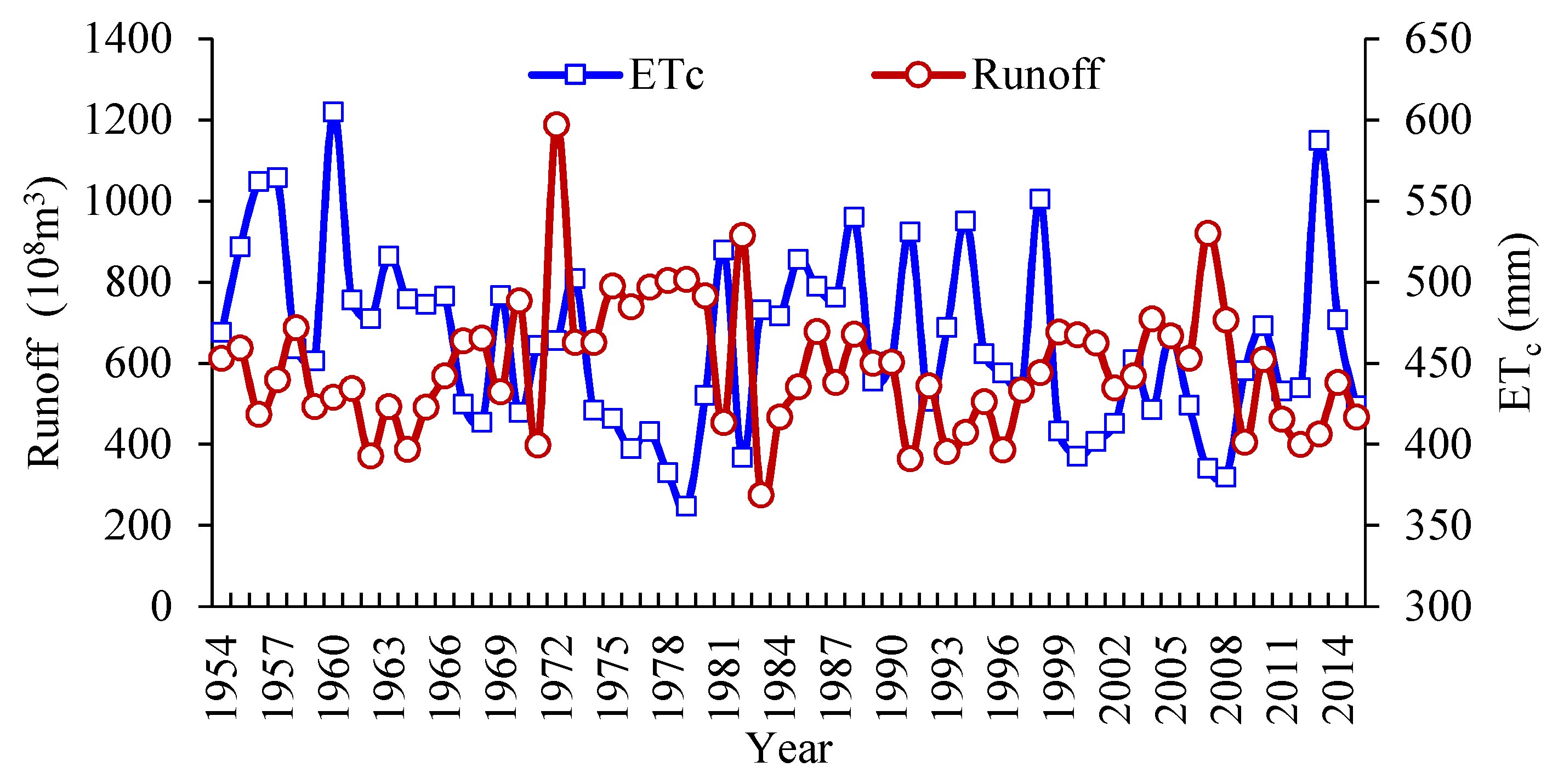
In order to determine the joint probability of water supply and water demand, data related water supply and demand were required. Surface water supply originated from the runoff of Songhua River, therefore, the runoff data of Songhua River at Jiamusi hydrometric station from 1954 to 2015 were collected. In this study, water demand was the numeric equivalent to the value of crop actual evapotranspiration (ETc). The actual evapotranspiration was calculated by multiplying the crop coefficient with reference evapotranspiration (ET0). Daily ET0 was estimated by the Penmen–Monteith formula [24] based on the meteorological data including wind speed, the highest temperature, the average temperature, the lowest temperature, relative humidity, and sunshine duration from national meteorological network. Monthly value of ET0 was obtained by the accumulation of the daily values. The crop coefficient of rice was: 0.38 for May, 0.78 for June, 1.335 for July, 1.06 for August, and 0.45 for September. Social-economic data involved in the optimization model were from the Feasibility Report of Jinxi Irrigation District, Yearbook of Fujin City and related references. Specifically, data related to different subareas are listed in Table 1. The emission per unit area of chemical oxygen demand, ammonia nitrogen, total nitrogen, and total phosphorus were 150 kg/ha, 11.85 kg/ha, 171.75 kg/ha, and 65.25 kg/ha, respectively, and the coefficient of chemical oxygen demand, ammonia nitrogen, total nitrogen, and total phosphorus that flow into the river were 0.06, 0.05, 0.04, and 0.01, respectively. The market price of rice was 3.16 RMB/kg, the planting cost of rice was 9589 RMB/ha, the price of irrigation water was 0.15 RMB/m3.
3.2. Parameter Estimation
Based on the runoff data of Jiamusi hydrometric station and the method for calculating crop ETc, the changes of runoff and ETc from 1954 to 2015 are depicted in Figure 2. In this study, the Pearson III distribution function was used to describe the hydrological distribution of runoff and ETc. Based on the maximum entropy principle for Pearson III distribution, the program was coded in MATLAB (MathWork, Natick, MA, USA) and the related parameters were estimated. The scale parameter, shape parameter and location parameter for annual runoff were 12.08, 3.47, and 14.97, respectively. Thus, the distribution of runoff was expressed as:
The scale parameter, shape parameter and location parameter for ETc were 15.27, 6.94, and 342.66, respectively. Thus, the distribution of ETc was expressed as:
These two distributions were considered as the marginal distributions of the joint distribution function of runoff and ETc.
3.3. Joint Probability of Water Supply and Water Demand
From Figure 2, the variability between runoff and ETc was obvious, leading to the necessity to obtain the joint probability of wet and dry conditions of these two random variables, thus guiding agricultural water resources allocation. Assume both runoff and ETc had three hydrological characteristics: wet, normal and dry conditions. In this study, the cumulative probability of wet and dry conditions were , . Specifically, for the wet condition: , for the normal condition: , and for the dry condition: , where X was the runoff volume or the value of ETc, and and were the critical values between wet and normal conditions, and between normal and dry conditions, respectively. Based on the above principle, there were in total nine scenario combination of runoff and ETc, i.e., wet (runoff) vs. wet (ETc), wet (runoff) vs. normal (ETc), wet (runoff) vs. dry (ETc), normal (runoff) vs. wet (ETc), normal (runoff) vs. normal (ETc), normal (runoff) vs. dry (ETc), dry (runoff) vs. wet (ETc), dry (runoff) vs. normal (ETc), and dry (runoff) vs. dry (ETc). Based on the marginal distribution functions of runoff and ETc, this study selected the commonly used Gaussian copula, t-copula, Archimedean copula (including Clayton copula, Frank copula, Gumbel copula, and Ali–Mikhail–Haq copula in this study which are frequently-used in hydrology-related analysis) to establish the joint distribution functions. The specific equations of these copula functions are presented in Appendix A. In this study, the Euclidean distance (), which is a non-probabilistic measure of goodness of approximation with the advantage of simple calculation [25,26], was used to evaluate the performance of each selected copula function. The value of was 0.042, 0.0411, 0.2037, 0.0402, 0.2037, and 0.3232 corresponding to the above copula functions. Results showed that the value of of Frank copula was the smallest, thus, the Frank copula was adopted and the joint distribution function of runoff and ETc could be expressed as [27]:
where U indicated the runoff, V indicated the ETc. In this study, .
Based on the joint distribution function, the contour of were drawn as Figure 3 shows, and the joint probabilities of each scenario was obtained. For example, the joint probability for the scenario of wet (runoff) vs. wet (ETc) was 1.6%, for the scenario of dry (runoff) vs. dry (ETc) was 1.63%, and for the scenario of normal (runoff) vs. normal (ETc) was 28.15%. The synchronous joint probability of runoff and ETc (31.38%) was appreciably lower than the asynchronous joint probability of runoff and ETc (68.62%). The runoff values corresponding to wet, normal, and dry conditions were 754.845 × 10⁸ m3, 604.136 × 10⁸ m3, and 474.903 × 10⁸ m3, respectively. The ETc values corresponding to wet, normal and dry conditions were 472.27 mm, 443.54 mm and 419.41 mm, respectively. The proportion of water supply for Jinxi irrigation district of the runoff volume from Jiamusi hydrometric station were 0.66% for wet condition, 0.7% for normal condition and 0.74% for dry condition. Therefore, the values of water supply and water demand under each scenario were obtained.
3.4. Agricultural Water Resource Allocation Schemes
According to the minimum deviation method, the optimization model was solved. The irrigation area was allocated to different subareas, then the water allocation amount can be obtained, based on the irrigation quota of different subareas, as shown in Figure 4. From the figure, it was obvious that if the wet and dry conditions of runoff were considered only, the water allocation amounts followed the law: wet > normal > dry conditions, indicating that a larger water supply would lead to a larger water allocation. If the wet and dry conditions of water demand were considered only, the water allocation amounts followed the law: dry > normal > wet conditions, indicating that a larger water demand would lead to a larger water allocation, because the value of water demand in the wet condition was the smallest, while it was the highestin the dry condition. Hence, two extreme conditions happened in the WD and DW scenarios between which DW indicated the most water shortage condition and should draw attention of policymakers, with the corresponding water allocation amount being 1.96 × 10⁸ m3. Based on the joint probabilities of different scenarios, the average water allocation level was obtained, i.e., 2.13 × 10⁸ m3. Such a result could provide a guidance in water resource planning of Jinxi irrigation district considering the combination of different scenarios. For different subareas, the change in the water allocation amount in Huama subarea was obvious because of its larger irrigation area. Based on the optimal results, the value of economic objective ranged from 8.32 × 10⁸ RMB to 12 × 108 RMB, with the average value under the nine scenarios being 9.55 × 10⁸ RMB. The value of social objective ranged from 3.29 × 10⁷ m3 to 7.13 × 10⁷ m3, with the average value under the nine scenarios being 5.05 × 10⁷ m3. The value of environmental objective ranged from 1.67 × 10⁶ kg to 2.39 × 10⁶ kg, with the average value under the nine scenarios being 1.91 × 10⁶ kg. These were the results of a comprehensive coordination of the three objectives.
3.5. Agricultural Water Resources Carrying Capacity
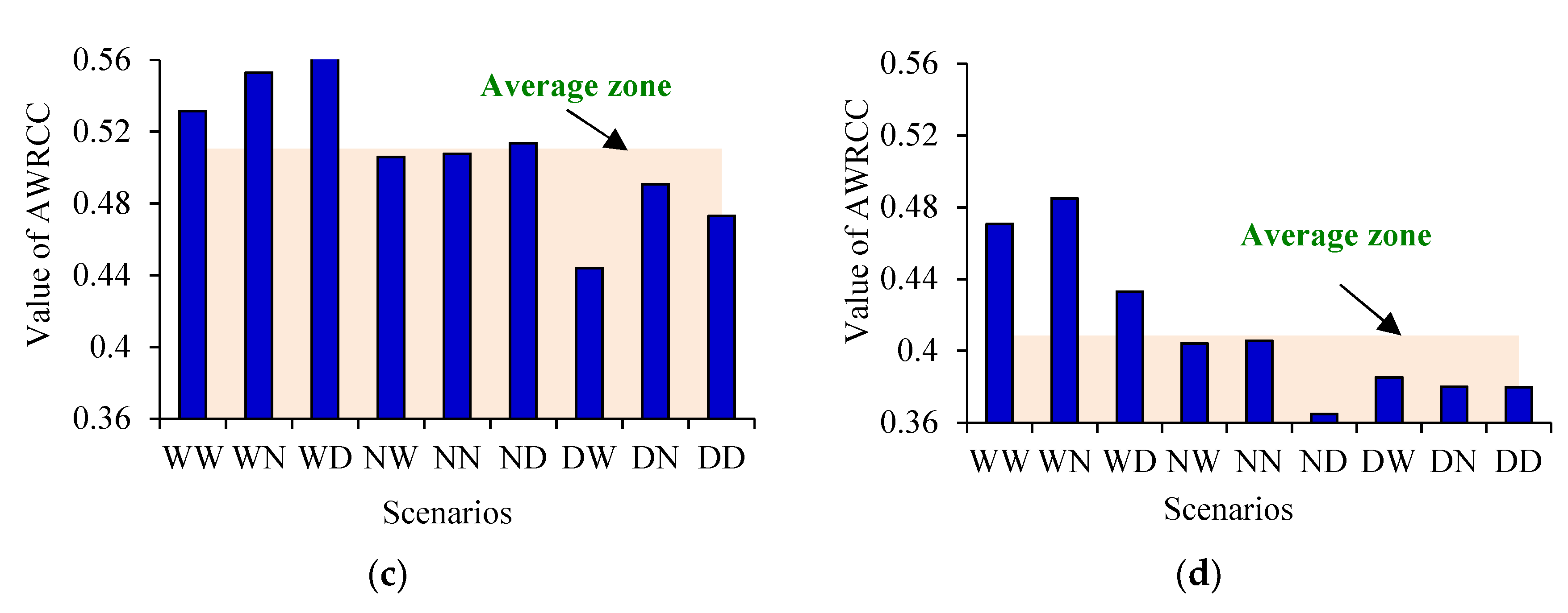
Based on the results of optimization model, the agricultural water resource carrying capacity was evaluated using the entropy-weight-based TOPSIS method. As the optimization model considered three objectives, involving economic, social, and environmental factors, the index system for evaluating agricultural water resources carrying capacity contained three dimensions, i.e., economic, social, and environmental dimensions, and each dimension contained three parameters. Detailed information of the index system can be found in Table 2. Acquisition of the values of these indices was based on the results of the optimization model and actual conditions. Using the entropy-weight method, the weight of each index was calculated as shown in Table 1. Based on the entropy-weight-based TOPSIS method, the agricultural water resources carrying capacity values for the four subareas were obtained as shown in Figure 5 This study divided the value of agricultural water resources carrying capacity into five grades: [0, 0.2) belonged to I grade, [0.2, 0.4) belonged to II grade, [0.4, 0.6) belonged to III grade, [0.6, 0.8) belonged to IV grade, and [0.8, 1.0) belonged to V grade. The larger the value the higher the grade, indicating the better the agricultural water resources carrying capacity. From Figure 5, the agricultural water resources carrying capacity in Toulin subarea was the worst with the average value of the nine scenarios being 0.41, and in Songhuajiang subarea it was the best with the average value of the nine scenarios being 0.52. However, the fluctuations of agricultural water resources carrying capacity for Huama subarea and Toulin subarea were obvious under different scenarios. This indicated that the agricultural water resources carrying capacity in these two subareas was sensitive to the changes of water supply and water demand. In general, the resources carrying capacity in the wet condition in terms of runoff was higher than that in the dry condition, indicating that the resources carrying capacity was more sensitive to water supply. Therefore, improving water use efficiency under the limited water supply was significant.
3.6. Discussion
Compared with traditional irrigation water allocation modes which were obtained based on “Water Resources Verification Report of Jinxi Irrigation District”, “Water Resources Argumentation Report of Jinxi Irrigation District”, and “Engineering Feasibility Study Report of Jinxi Irrigation District”, one of the main contributions of this study was to consider the changes of water supply and water demand as well as their interrelationships. For this, we established the joint distribution function of water supply and water demand, based on which, different scenarios with the combination of wet and dry conditions of water supply and water demand were generated. This would provide decision makers more reasonable references for irrigation water allocation. Additionally, this could help decision-makers for irrigation water allocation to response promptly to different changes in natural conditions, andimprove the adaption ability to climate change. Another major contribution of this study was that multiple targets were considered when optimally allocating limited water resources, including economic, social and environmental aspects. This avoided the disadvantage of traditional irrigation water allocation patterns of the study area that focused on economic benefit. (In the related reports as mentioned above, the current irrigation water allocation plans for crops were based on the benefit-cost analysis, without analyzing the associated social and environmental impacts). Compared with actual conditions of the study area, taking the normal-normal scenario of water supply and water demand which was the scenario that was the most likely to happen (with the joint probability was 28.15%) as an example, the optimal results could save 0.57 × 10⁸ m3 water resources. From the angle of environmental protection, the optimal results could reduce pollutants emission of 5.14 × 10⁵ kg. Such results were conducive to improve the efficiency and sustainability of irrigation water allocation. Moreover, the agricultural water resource carrying capacity was evaluated based on the optimal results to help decision makers evaluate the irrigation strategies under different scenarios and, thus, provide guidance when planning the irrigation water of the irrigation district. The major limitation of this study was that the dynamics of the framework was ignored, for example, the changes of water supply and demand during the crop growth period and the changes in crop growth factors were not considered, which might affect the applicability of the proposed framework. Future work would make it a priority to improve the proposed framework.
4. Conclusions
This study developed a framework for agricultural water resources management, including the determination of the distribution function of water supply and water demand based on parameter estimation, joint probability of water supply and water demand, optimization model for agricultural water resources allocation, and evaluation of agricultural water resources carrying capacity. The relationship between the adjacent components is input-output. Specifically, because of the characteristic of high accuracy and quick calculation, the maximum entropy methodis used to estimate the parameters of the probability distributions of water supply and water demand, so that the joint probabilities of these two random variables can be obtained based on the copula function. Thus, nine scenarios with the combination of wet and dry conditions of water supply and water demand are generations, and agricultural water resources is optimally allocated under these scenarios, considering the comprehensive benefit of economic, social, and environmental dimensions. The results can provide decision makers more alternatives of water allocation schemes considering the changes of natural conditions, which is conducive to agricultural water planning. Lastly, agricultural water resources carrying capacity is evaluated based on the optimal results using entropy-weight-based TOPSIS methods, which can avoid the subjectivity of weight determination, and objectively and thoroughly reflect the trend of dynamic change of agricultural water resources carrying capacity.
The developed framework is applied to a real case study in an irrigation district in northeast China. Results demonstrated the feasibility and applicability of using the maximum entropy method and entropy-weight-based TOPSIS method to agricultural water resources management, and the results can provide a certain guidance for local agricultural water management. The developed framework and the associated method can also be applied to regional resources management problem or to other regions. This study aims to construct such a framework for agricultural water resources management, however, concrete details for some components are simplified, for example, the objective functions and constraints of optimization model are simple with only basic elements associated with economic, social, and environmental aspects being considered, and the dynamics of the framework are overlooked. These deserves further study to improve the framework.
Author Contributions
Conceptualization: M.L.; data curation: H.S.; formal analysis: H.S.; funding acquisition: M.L. and Y.Z.; methodology: M.L., H.S., and Y.Z.; resources: Y.Z.; software: M.M.; writing—original draft: M.L.; writing—review and editing: V.P.S.
Funding
This research was funded by the Natural Science Foundation of Heilongjiang Province of China (E2018004, E2016005), the National Natural Science Foundation of China (51809040, 41701022), and Humanity and Social Science general project of Ministry of Education of China (18YJAZH147).
Conflicts of Interest
The authors declare no conflict of interest.
Appendix A

Table A1.
Equations of the copula functions in this study.
| Function Name | Interpretation | |
|---|---|---|
| Gaussian copula | is the inverse function of standard normal distribution function; is the correlation coefficients between variables. | |
| t-copula | is the inverse function t distribution function with the degree of freedom is k; is the correlation coefficients between variables. | |
| Clayton copula | and . is the Kendall coefficient of rank correlation, and the same below. | |
| Frank copula | and | |
| Gumbel copula | and | |
| Ali–Mikhail–Haq copula | and |
References
- Dai, Z.Y.; Li, Y.P. A multistage irrigation water allocation model for agricultural land-use planning under uncertainty. Agric. Water Manag. 2013, 129, 69–79. [Google Scholar] [CrossRef]
- Li, M.; Fu, Q.; Singh, V.P.; Liu, D. An interval multi-objective programming model for irrigation water allocation under uncertainty. Agric. Water Manag. 2018, 196, 24–36. [Google Scholar] [CrossRef]
- Li, M.; Fu, Q.; Singh, V.P.; Ma, M.W.; Liu, X. An intuitionistic fuzzy multi-objective non-linear programming model for sustainable irrigation water allocation under the combination of wet and dry conditions. J. Hydrol. 2017, 555, 80–94. [Google Scholar] [CrossRef]
- Feng, Y.; Cui, N.B.; Gong, D.Z.; Zhang, Q.W.; Zhao, L. Evaluation of random forests and generalized regression neural networks for daily reference evapotranspiration modelling. Agric. Water Manag. 2017, 193, 163–173. [Google Scholar] [CrossRef]
- Yu, Y.H.; Zhang, H.B.; Singh, V.P. Forward prediction of runoff data in data-scarce basins with an improved ensemble empirical model decomposition (EEMD) model. Water 2018, 10, 388. [Google Scholar] [CrossRef]
- Zhang, L.; Singh, V.P. Bivariate Flood Frequency Analysis Using the Copula Method. J. Hydrol. Eng. 2006, 11, 150–164. [Google Scholar] [CrossRef]
- Hao, Z.; Singh, V.P. Modeling multisite streamflow dependence with maximum entropy copula. Water Resour. Res. 2013, 49, 7139–7143. [Google Scholar] [CrossRef] [Green Version]
- Salvadori, G.; Durante, F.; De Michele, C.; Bernardi, M.; Petrella, L. A multivariate copula-based framework for dealing with hazard scenarios and failure probabilities. Water Resour. Res. 2016, 52, 3701–3721. [Google Scholar] [CrossRef]
- Zhang, J.P.; Lin, X.M.; Guo, B.T. Multivariate copula-based joint probability distribution of water supply and demand in irrigation district. Water Resour. Manag. 2016, 30, 2361–2375. [Google Scholar] [CrossRef]
- Golian, S.; Farokhnia, A.; Saghafian, B. Copula-based interpretation of continuous rainfall–runoff simulations of a watershed in northern Iran. Can. J. Earth Sci. 2012, 49, 681–691. [Google Scholar] [CrossRef]
- Chen, L.; Singh, V.P. Entropy-based derivation of generalized distributions for hydrometeorological frequency analysis. J. Hydrol. 2018, 557, 699–712. [Google Scholar] [CrossRef]
- Cui, H.; Singh, V.P. Application of minimum relative entropy theory for streamflow forecasting. Stoch. Environ. Res. Risk Assess. 2017, 31, 587–608. [Google Scholar] [CrossRef]
- Singh, V.P. Entropy-Based Parameter Estimation in Hydrology; Kluwer Academic Publishers: Boston, MA, USA; London, UK, 1998. [Google Scholar]
- Li, M.; Fu, Q.; Guo, P.; Singh, V.P.; Zhang, C.L.; Yang, G.Q. Stochastic multi-objective decision making for sustainable irrigation in a changing environment. J. Clean. Prod. 2019, 223, 928–945. [Google Scholar] [CrossRef]
- Ren, C.F.; Li, Z.H.; Zhang, H.B. Integrated multi-objective stochastic fuzzy programming and AHP method for agricultural water and land optimization allocation under multiple uncertainties. J. Clean. Prod. 2019, 210, 12–24. [Google Scholar] [CrossRef]
- Li, M.; Fu, Q.; Singh, V.P.; Ji, Y.; Liu, D.; Zhang, C.L.; Li, T.X. An optimal modelling approach for managing agricultural water-energy-food nexus under uncertainty. Sci. Total. Environ. 2019, 651, 1416–1434. [Google Scholar] [CrossRef]
- Roy, T.; Dutta, R.K. Integrated fuzzy AHP and fuzzy TOPSIS methods for multi-objective optimization of electro discharge machining process. Soft Comput. 2018, 1–11. [Google Scholar] [CrossRef]
- Wang, Z.-X.; Li, D.-D.; Zheng, H.-H. The External Performance Appraisal of China Energy Regulation: An Empirical Study Using a TOPSIS Method Based on Entropy Weight and Mahalanobis Distance. Int. J. Environ. Res. Public Health 2018, 15, 236. [Google Scholar] [CrossRef] [PubMed]
- Wang, S.F.; Singh, V.P. Spatio-Temporal Variability of Soil Water Content under Different Crop Covers in Irrigation Districts of Northwest China. Entropy 2017, 19, 410. [Google Scholar] [CrossRef]
- Sonuga, J.O. Principle of maximum entropy in hydrologic frequency analysis. J. Hydrol. 1972, 17, 177–191. [Google Scholar] [CrossRef]
- Zhang, L.; Singh, V.P. Bivariate Rainfall and Runoff Analysis Using Entropy and Copula Theories. Entropy 2012, 14, 1784–1812. [Google Scholar] [CrossRef] [Green Version]
- Li, M.; Guo, P. A multi-objective optimal allocation model for irrigation water resources under multiple uncertainties. Appl. Math. Model. 2014, 38, 4897–4911. [Google Scholar] [CrossRef]
- Chung, E.; Abdulai, P.J.; Park, H.; Kim, Y.; Ahn, S.R.; Kim, S.J. Multi-criteria assessment of spatial robust water resource vulnerability using the TOPSIS method coupled with objective and subjective weights in the Han River Basin. Sustainability 2017, 9, 29. [Google Scholar] [CrossRef]
- Allen, R.G.; Pereira, L.S.; Raes, D.; Smith, M. Crop Evapotranspiration: Guideline for Computing Crop Water Requirement; FAO Irrigation and Drainage paper 56; FAO: Rome, Italy, 1998. [Google Scholar]
- Dong, S.; Wang, N.N.; Lu, H.M.; Tang, L.J. Bivariate distributions of group height and length for ocean waves using Copula methods. Coast. Eng. 2015, 96, 49–61. [Google Scholar] [CrossRef]
- Yu, J.; Feng, Q.; Li, Y.; Cao, J.D. Stochastic Optimal Dispatch of Virtual Power Plant considering Correlation of Distributed Generations. Math. Probl. Eng. 2015, 2015, 1–8. [Google Scholar] [CrossRef]
- Zhang, L.; Singh, V.P. Bivariate rainfall frequency distributions using Archimedean copulas. J. Hydrol. 2007, 332, 93–109. [Google Scholar] [CrossRef]
Figure 1.
Framework for agricultural water resources management.

Figure 2.
Changes of runoff and ETc.

Figure 3.
Joint probability of runoff (U) and ETc (V).

Figure 4.
Water allocation for different subareas under different scenarios. (Note: (1) W—wet, N—normal, D—dry; (2) the first letter indicates the conditions of runoff and the second letter indicates the conditions of ETc; (3) the number inside the box means the total water allocation amount of different scenarios; and (4) the red dashed line is the average value of different scenarios).

Figure 5.
Agricultural water resource carrying capacity for different subareas. (a) Songhuajiang; (b) Jinshan; (c) Huama; and (d) Toulin. (Note: AWRCC means agricultural water resource carrying capacity).
Figure 5.
Agricultural water resource carrying capacity for different subareas. (a) Songhuajiang; (b) Jinshan; (c) Huama; and (d) Toulin. (Note: AWRCC means agricultural water resource carrying capacity).


Table 1.
Data related to different subareas.
| Parameter | Unit | Subarea | |||
|---|---|---|---|---|---|
| Songhuajiang | Jinshan | Huama | Toulin | ||
| Yield per unit area | kg/ha | 8465.67 | 8511.17 | 8511.17 | 7887.33 |
| Irrigation quota | m3/ha | 3660.33 | 3686.48 | 3686.48 | 3327.95 |
| Population | 104 people | 0.77 | 4.31 | 1.12 | 1.62 |
| Maximum irrigation area | 104 ha | 0.53 | 1.85 | 3.34 | 2.28 |
| Minimum irrigation area | 104 ha | 0.51 | 1.225 | 1.85 | 1.43 |
Table 2.
Index system and weights.
| Dimension | Index | Calculation Formula | Unit | Index Attribute | Weights |
|---|---|---|---|---|---|
| Economic dimension (A) | Water production efficiency (A1) | Yield/(Crop evapotranspiration) | kg/ha | + | 0.1013 |
| Production value per unit water (A2) | (Yield per unit water) × Market price | RMB/m3 | + | 0.1095 | |
| Grain output (A3) | Yield × (Market price) | RMB | + | 0.1018 | |
| Social dimension (B) | Food per capita (B1) | Yield/Population | kg/capita | + | 0.1443 |
| Water per capita (B2) | Water resource amount/Population | m3/capita | + | 0.0923 | |
| Agricultural water shortage (B3) | (Crop evapotranspiration-Irrigation amount) × Irrigation area | m3 | − | 0.1393 | |
| Environmental dimension (C) | Agricultural non-point pollution discharge (C1) | (Emission of agricultural non-point pollution per unit area) × Planting area | kg | − | 0.0996 |
| Agricultural greenhouse gases emission (C2) | (Emission of agricultural greenhouse gases per unit area) × Planting area | kg | − | 0.0997 | |
| Coefficient of groundwater exploitation (C3) | (Groundwater exploitation amount)/(Total groundwater amount) | % | − | 0.1122 |
Note: “+” indicates the index belongs to the attribute of “the larger, the better”, while “−” indicates the index belongs to the attribute of “the smaller, the better”.
© 2019 by the authors. Licensee MDPI, Basel, Switzerland. This article is an open access article distributed under the terms and conditions of the Creative Commons Attribution (CC BY) license (http://creativecommons.org/licenses/by/4.0/).
Share and Cite
MDPI and ACS Style
Li, M.; Sun, H.; Singh, V.P.; Zhou, Y.; Ma, M. Agricultural Water Resources Management Using Maximum Entropy and Entropy-Weight-Based TOPSIS Methods. Entropy 2019, 21, 364. https://0-doi-org.brum.beds.ac.uk/10.3390/e21040364
AMA Style
Li M, Sun H, Singh VP, Zhou Y, Ma M. Agricultural Water Resources Management Using Maximum Entropy and Entropy-Weight-Based TOPSIS Methods. Entropy. 2019; 21(4):364. https://0-doi-org.brum.beds.ac.uk/10.3390/e21040364
Chicago/Turabian StyleLi, Mo, Hao Sun, Vijay P. Singh, Yan Zhou, and Mingwei Ma. 2019. "Agricultural Water Resources Management Using Maximum Entropy and Entropy-Weight-Based TOPSIS Methods" Entropy 21, no. 4: 364. https://0-doi-org.brum.beds.ac.uk/10.3390/e21040364
Note that from the first issue of 2016, this journal uses article numbers instead of page numbers. See further details here.