Ordinal Pattern Based Entropies and the Kolmogorov–Sinai Entropy: An Update

Abstract

Different authors have shown strong relationships between ordinal pattern based entropies and the Kolmogorov–Sinai entropy, including equality of the latter one and the permutation entropy, the whole picture is however far from being complete. This paper is updating the picture by summarizing some results and discussing some mainly combinatorial aspects behind the dependence of Kolmogorov–Sinai entropy from ordinal pattern distributions on a theoretical level. The paper is more than a review paper. A new statement concerning the conditional permutation entropy will be given as well as a new proof for the fact that the permutation entropy is an upper bound for the Kolmogorov–Sinai entropy. As a main result, general conditions for the permutation entropy being a lower bound for the Kolmogorov–Sinai entropy will be stated. Additionally, a previously introduced method to analyze the relationship between permutation and Kolmogorov–Sinai entropies as well as its limitations will be investigated.

1. Introduction

The Kolmogorov–Sinai entropy is a central measure for quantifying the complexity of a measure-preserving dynamical system. Although it is easy from the conceptional viewpoint, its determination and its estimation from given data can be challenging. Since Bandt, Keller, and Pompe showed the coincidence of Kolmogorov–Sinai entropy and permutation entropy for interval maps (see [1]), there have been different attempts to approach the Kolmogorov–Sinai entropy by ordinal pattern based entropies (see e.g., [2,3,4,5,6] and references therein), leading to a nice subject of study. In this paper, we want to discuss the relationship of the Kolmogorov–Sinai entropy to the latter kind of entropies. We respond to the state of the art and give some generalizations and new results, mainly emphasizing combinatorial aspects.

For this, let $(\Omega ,\mathcal{A},\mu ,T)$ be a measure-preserving dynamical system, which we think to be fixed in the whole paper. Here, $(\Omega ,\mathcal{A},\mu )$ is a probability space equipped with a $\mathcal{A}$-$\mathcal{A}$- measurable map $T:\Omega \to \Omega$ satisfying $\mu \left(T^{-1}\left(A\right)\right)=\mu \left(A\right)$ for all $A\in \mathcal{A}$. Certain properties of the system will be specified at the places where they are of interest. It is suggested for the following to interpret $\Omega$ as the set of states of a system, $\mu$ as their distribution, and T as a description of the dynamics underlying the system and saying that the system is in state $T\left(\omega \right)$ at time $t+1$ if it is in state $\omega \in \Omega$ at time t.

In the following, we give the definitions of the central entropies considered in this paper.

1.1. The Kolmogorov–Sinai Entropy

The base of quantifying dynamical complexity is to consider the development of partitions and their entropies under the given dynamics. Recall that the coarsest partitions refining given partitions ${\mathcal{P}}_1,{\mathcal{P}}_2,\dots ,{\mathcal{P}}_k$ and $\mathcal{P},\mathcal{Q}$ of $\Omega$ are defined by

$$\underset{s=1}{\overset{k}{\bigvee }}{\mathcal{P}}_s:=\left\{\bigcap _{s=1}^k{P}_s\ne \varnothing \mid P_s\in {\mathcal{P}}_s \mathrm{for} s=1,2,\dots ,k\right\}$$

and

$$\mathcal{P}\vee \mathcal{Q}:=\{P\cap Q\ne \varnothing \mid P\in \mathcal{P},Q\in \mathcal{Q}\},$$

respectively. The entropy of a finite or countably infinite partition $\mathcal{Q}\subset \mathcal{A}$ of $\Omega$ is given by

$$H\left(\mathcal{Q}\right):=-\sum _{Q\in \mathcal{Q}}\mu \left(Q\right)log\mu \left(Q\right).$$

For a finite or countably infinite partition $\mathcal{P}:={\left\{P_i\right\}}_{i\in I}\subset \mathcal{A}$ of $\Omega$ and some $k\in \mathbb{N}$, consider the partition

$${\mathcal{P}}^{\left(k\right)}:=\underset{t=0}{\overset{k-1}{\bigvee }}{T}^{-t}\left(\mathcal{P}\right)=\{P\left(\mathit{i}\right)\ne \varnothing \mid \mathit{i}\in I^k\},$$

where

$$P\left(\mathit{i}\right):=\bigcap _{t=0}^{k-1}{T}^{-t}\left(P_{i_t}\right)$$

for each multiindex $\mathit{i}=(i_0,i_1,\dots ,i_{k-1})\in I^k$. The entropy rate of T with regard to a finite or countably infinite partition $\mathcal{P}\subset \mathcal{A}$ with $H\left(\mathcal{P}\right)<\infty$ is defined by

$$h\left(\mathcal{P}\right):=\underset{n\to \infty }{lim}\frac{1}{n}H\left({\mathcal{P}}^{\left(n\right)}\right).$$

The Kolmogorov–Sinai entropy is then defined as

$$\mathrm{KS}:=\underset{\mathcal{P}}{sup}h\left(\mathcal{P}\right),$$

where the supremum is taken over all finite or over all countably finite partitions $\mathcal{P}\subset \mathcal{A}$ with $H\left(\mathcal{P}\right)<\infty$.

1.2. Ordinal Pattern Based Entropy Measures

As the determination and estimation of the Kolmogorov–Sinai entropy based on the given definition are often not easy, there are many different alternative approaches to it, among them the permutation entropy approach by Bandt and Pompe [7]. The latter is built up on the concept of ordinal patterns, which we describe in a general manner now.

For this, let $\mathit{X}=(X_1,X_2,\dots ,X_d):\Omega \to {\mathbb{R}}^d$ be a random vector for $d\in \mathbb{N}$. Here, each of the random variables $X_i$ can be interpreted as an observable measuring some quantity in the following sense: If the system is in state $\omega$ at time 0, then the arschvalue of the quantity mesured at time t provides $X_i\left(T^t\left(\omega \right)\right)$. This general approach includes the one-dimensional case that states and measurements coincide, and this is that $\Omega \subseteq \mathbb{R}$ and $\mathit{X}=id$ is the identical map on $\Omega$. This case, originally considered in [7] and subsequent papers, is discussed in Section 3. We refer to it as the simple one-dimensional case.

Let

$${\Pi }_n:=\{(r_0,r_1,\dots r_{n-1})\in {\{0,1,\dots n-1\}}^n\mid r_i\ne r_j\mathrm{for}i\ne j\}$$

be the set of all permutations of length n. We say that a vector $(x_0,x_1,\dots ,x_{n-1})\in {\mathbb{R}}^n$ has ordinal pattern $\pi =(r_0,r_1,\dots r_{n-1})\in {\Pi }_n$ if

$$x_{r_{i-1}}<x_{r_i}\mathrm{or}{x}_{r_{i-1}}=x_{r_i}\mathrm{and}{r}_i<r_{i-1}$$

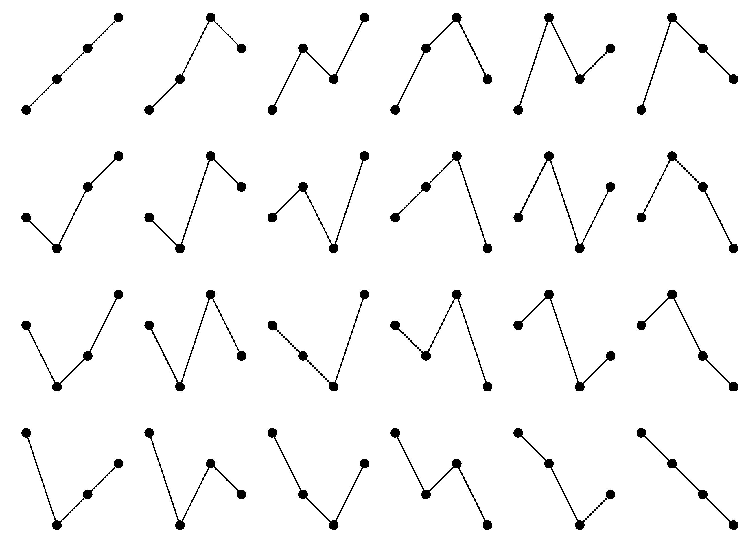
holds true for all $i\in \{1,2\dots ,n-1\}$. The $n!$ possible ordinal patterns (compare Figure 1) provide a classification of the vectors. We denote the set of points with ordinal pattern ${\pi }_1,{\pi }_2,\dots ,{\pi }_d\in {\Pi }_n$ with regard to $X_1,X_2,\dots ,X_d$, respectively, by

$$\begin{array}{c}{P}_{{\pi }_1,{\pi }_2,\dots ,{\pi }_d}^{\mathbf{X}}\hfill \\ =\left\{\omega \in \Omega \mid \left(X_i\left(\omega \right),X_i\left(T\left(\omega \right)\right),\dots ,X_i\left(T^{n-1}\left(\omega \right)\right)\right)\mathrm{has}\mathrm{ordinal}\mathrm{pattern}{\pi }_i\mathrm{for}i=1,2,\dots ,d\right\}\hfill \end{array}$$

and by

$$O{P}^{\mathit{X}}\left(n\right):=\left\{P_{{\pi }_1,{\pi }_2,\dots ,{\pi }_d}^{\mathbf{X}}:\ne \varnothing \mid {\pi }_1,{\pi }_2,\dots ,{\pi }_d\in {\Pi }_n\right\}$$

the partition of $\Omega$ into those sets.

We are especially interested in three ordinal pattern based entropy measures. These are the lower and upper permutation entropies defined as

$${\underline{\mathrm{PE}}}^{\mathbf{X}}=\underset{n\to \infty }{lim\; inf}\frac{1}{n}H\left(O{P}^{\mathit{X}}\left(n\right)\right)$$

and

$${\overline{\mathrm{PE}}}^{\mathbf{X}}=\underset{n\to \infty }{lim\; sup}\frac{1}{n}H\left(O{P}^{\mathit{X}}\left(n\right)\right),$$

respectively, and the conditional entropy of ordinal patterns defined by

$${\mathrm{CE}}^{\mathbf{X}}=\underset{n\to \infty }{lim\; inf}\left[H\left({\left(O{P}^{\mathit{X}}\left(n\right)\right)}^{\left(2\right)}\right)-H\left(O{P}^{\mathit{X}}\left(n\right)\right)\right].$$

We speak of the permutation entropy if the upper and lower permutation entropies coincide.

1.3. Outline of This Paper

In Section 2, we will focus on the relationship between permutation and Kolmogorov–Sinai entropies in the general setting. With Theorems 1 and 3, we will restate two known statements. A new proof of Theorem 1 will be given in Appendix A.2. Theorem 3 is stated for completeness. Theorem 2 establishes a new relationship between the conditional permutation entropy and the Kolmogorov–Sinai entropy.

In Section 3, the relationship between permutation and Kolmogorov–Sinai entropies in the one-dimensional case is investigated. Conditions are introduced, under which the permutation entropy is equal to the Kolmogorov–Sinai entropy. The given conditions allow for a generalization of previous results. We will explain why (countably) piecewise monotone functions satisfy these conditions and consider two examples.

In Section 4, we will investigate a method to analyze the relationship between permutation and Kolmogorov–Sinai entropies that was first introduced in [5]. We will use this method to relate two different kinds of conditional permutation entropies in the general setting. Theorem 5 shows that this method cannot be used directly to prove equality between permutation and Kolmogorov–Sinai entropies.

The results of the paper are summarized in Section 5. The proofs for all new results can be found in the Appendix A.

2. Relating Entropies

2.1. Partitions via Ordinal Patterns

Given some $d,n\in \mathbb{N}$ and some random vector $\mathit{X}=(X_1,X_2,\dots ,X_d)$, the partition described above can be defined in an alternative way, which is a bit more abstract but better fitting for the approach used in the proof of Theorem 4:

We can determine to which set $P_{\pi }\in O{P}^{X_i}\left(n\right)$ a point $\omega \in \Omega$ belongs to if we know whether $X_i\left(T^s\left(\omega \right)\right)<X_i\left(T^t\left(\omega \right)\right)$ holds true for all $s,t\in \{0,1,\dots ,n-1\}$ with $s<t$. Therefore, we can write

$$O{P}^{X_i}\left(n\right)=\underset{s=0}{\overset{n-1}{\bigvee }}\underset{t=s+1}{\overset{n-1}{\bigvee }}\left\{\left\{\omega \in \Omega \mid X_i\left(T^s\left(\omega \right)\right)<X_i\left(T^t\left(\omega \right)\right)\right\},\left\{\omega \in \Omega \mid X_i\left(T^s\left(\omega \right)\right)\ge X_i\left(T^t\left(\omega \right)\right)\right\}\right\}.$$

Throughout this paper, we will use the set

$$R:=\{(x,y)\in {\mathbb{R}}^2\mid x<y\}$$

to describe the order relation between two points. This notation allows us to write

$$O{P}^{\mathit{X}}\left(n\right)=\underset{i=1}{\overset{d}{\bigvee }}\underset{s=0}{\overset{n-1}{\bigvee }}\underset{t=s+1}{\overset{n-1}{\bigvee }}{(T^s,T^t)}^{-1}\left({(X_i\times X_i)}^{-1}\left(\{R,{\mathbb{R}}^2\backslash R\}\right)\right).$$

2.2. Ordinal Characterization of the Kolmogorov–Sinai Entropy

To be able to reconstruct all information of the given system via quantities based on the random vector $\mathit{X}=(X_1,X_2,\dots ,X_d)\to {\mathbb{R}}^d$, we need to assume that the latter itself does not reduce information. From the mathematical viewpoint, this means that the $\sigma$-algebra generated by $\mathit{X}$ is equivalent to the originally given $\sigma$-algebra $\mathcal{A}$, i.e., that

$$\sigma \left(\left\{X_i\circ T^t\mid t\in {\mathbb{N}}_0,i\in \{1,2,\dots ,d\}\right\}\right)\stackrel{\mu }{=}\mathcal{A}$$

(1)

holds true, which is roughly speaking that orbits are separated by the given random vector. For definitions and some more details concerning $\sigma$-algebras and partitions, see Appendix A.1.

The following statement saying that, under (1), ordinal patterns entailing the complete information of the given system have been shown in [3] in a s slightly weaker form than given here.

Theorem 1.

Let $\mathit{X}:\Omega \to {\mathbb{R}}^d$ be a random vector satisfying (1). Then,

$${\underline{\mathrm{PE}}}^{\mathbf{X}}\ge \underset{k\to \infty }{lim}h\left(O{P}^{\mathit{X}}\left(k\right)\right)=\mathrm{KS}$$

(2)

holds true.

Note that the inequality in (2) is a relatively simple fact: Since the partition $O{P}^{\mathit{X}}\left(n\right)$ is finer than the partition ${\left(O{P}^{\mathit{X}}\left(k\right)\right)}^{(n-k)}$ for all $n\ge k$, we have

$$H\left(O{P}^{\mathit{X}}\left(n\right)\right)\ge H\left({\left(O{P}^{\mathit{X}}\left(k\right)\right)}^{(n-k)}\right).$$

Dividing both sides by n and taking n and subsequently k to infinity proves this inequality.

Proofs of the inequality ${\underline{\mathrm{PE}}}^{\mathbf{X}}\ge \mathrm{KS}$ are also implicitly given in [1,8]. One-dimensional systems with direct observation as considered there are discussed in Section 3 in detail.

We will give a proof of the equality in (2) in Appendix A.2 being alternative to that in [3].

2.3. Conditional Entropies

In the case that (1) holds and that $\mathrm{KS}$ and ${\underline{\mathrm{PE}}}^{\mathbf{X}}$ coincide, in Appendix A.3, we will prove different representations of the Kolmogorov–Sinai entropy by ordinal pattern based conditional entropies as they are given in the following theorem.

Theorem 2.

Let $\mathit{X}:\Omega \to {\mathbb{R}}^d$ be a random vector satisfying (1). If $\mathrm{KS}\ge {\overline{\mathrm{PE}}}^{\mathbf{X}}$ is true, then

$$\begin{array}{cc}\mathrm{KS}\hfill & =\underset{n\to \infty }{lim\; inf}H\left(O{P}^{\mathit{X}}\left(n\right)\mid T^{-1}\left({\left(O{P}^{\mathit{X}}\left(n\right)\right)}^{\left(k\right)}\right)\right)\hfill \\ \hfill & =\underset{n\to \infty }{lim\; inf}H\left({\left(O{P}^{\mathit{X}}\left(n+1\right)\right)}^{\left(k\right)}\mid {\left(O{P}^{\mathit{X}}\left(n\right)\right)}^{\left(k\right)}\right)\hfill \\ \hfill & ={\underline{\mathrm{PE}}}^{\mathbf{X}}={\overline{\mathrm{PE}}}^{\mathbf{X}}\hfill \end{array}$$

holds true for all $k\in \mathbb{N}$, in particular, in the case $k=1$, one has $\mathrm{KS}={\mathrm{CE}}^{\mathbf{X}}={\underline{\mathrm{PE}}}^{\mathbf{X}}={\overline{\mathrm{PE}}}^{\mathbf{X}}$.

2.4. Amigó’S Approach

Amigó et al. [2,8] describe an alternative ordinal way to the Kolmogorov–Sinai entropy, which is based on a refining sequence of finite partitions. We present it in a slightly more general manner as originally given and in the language of finite-valued random variables. Note that the basic result behind Amigo’s approach in [2,8] is that the Kolmogorov–Sinai entropy of a finite alphabet source and its permutation entropy given some order on the alphabet coincide (see also [9] for an alternative algebraic proof of the statement).

Theorem 3.

Given a sequence ${\left(X_k\right)}_{k\in \mathbb{N}}$ of $\mathbb{R}$-valued random variables satisfying

(i) 

$\#\left(X_k(\Omega )\right)<\infty$ for all $k\in \mathbb{N}$,

(ii) 

$\sigma \left(X_k\right)\subseteq \sigma \left(X_{k+1}\right)$ for all $k\in \mathbb{N}$,

(iii) 

$\sigma \left(\{X_k\mid k\in \mathbb{N}\}\right)\stackrel{\mu }{=}\mathcal{A}$,

then it holds

$$\underset{k\to \infty }{lim}{\underline{\mathrm{PE}}}^{X_k}=\mathrm{KS}.$$

3. The Simple One-Dimensional Case

In the following, we consider the case that $\Omega$ is a subset of $\mathbb{R}$ with $\mathcal{A}$ coinciding with the Borel $\sigma$-algebra $\mathcal{B}$ on $\Omega$, and with $\mathit{X}=id$ being the identical map on $\Omega$. The $\mathit{X}$ is superfluous here, which is why we leave out each superscript $\mathit{X}$. For example, we write $OP\left(n\right)$ instead of $O{P}^{id}\left(n\right)$.

3.1. (Countably) Piecewise Monotone Maps

We discuss some generalization of the results of Bandt, Keller, and Pompe that Kolmogorov–Sinai entropy and permutation entropy coincide for interval maps (see [1]) on the basis of a statement given in the paper [10]. The discussion sheds some light on structural aspects of the proofs given in that paper with some potential for further generalizations.

Definition 1.

Let Ω be a subset of $\mathbb{R}$ and $\mathcal{B}$ be the Borel σ-algebra on Ω and μ be a probability measure on $(\Omega ,\mathcal{B})$. Then, we call a partition $\mathcal{M}={\left\{M_i\right\}}_{i\in I}$ of Ω ordered (with regard to μ), if $\mathcal{M}\subset \mathcal{B}$ and

$${\mu }^2\left((M_{i_1}\times M_{i_2})\cap R\right)\in \left\{0,{\mu }^2(M_{i_1}\times M_{i_2})\right\}$$

(3)

holds true for all $i_1,i_2\in I$ with $i_1\ne i_2$. Here, ${\mu }^2$ denotes the product measure of μ with itself.

We call a map $T:\Omega \to \Omega$ (countably) piecewise monotone (with regard to μ) if there exists a finite (or countably infinite) ordered partition $\mathcal{M}={\left\{M_i\right\}}_{i\in I}$ of Ω with $H\left(\mathcal{M}\right)<\infty$ such that

$${\mu }^2\left((M_i\times M_i)\cap R\cap {(T\times T)}^{-1}\left(R\right)\right)\in \left\{0,{\mu }^2\left((M_i\times M_i)\cap R\right)\right\}$$

(4)

holds true for all $i\in I$.

Given a probability space $(\Omega ,\mathcal{A},\mu )$, for two families of sets $\mathcal{P},\mathcal{Q}\subseteq \mathcal{A}$, we write

$$\mathcal{P}\prec \mathcal{Q}$$

if, for all $Q\in \mathcal{Q}$, there exists a $P\in \mathcal{P}$ with $\mu (Q\backslash P)=0$. If $\mathcal{P}={\left\{P_i\right\}}_{i\in I}$ and $\mathcal{Q}={\left\{Q_j\right\}}_{j\in J}$ are partitions of $\Omega$ in $\mathcal{A}$, $\mathcal{P}\prec \mathcal{Q}$ is equivalent to the fact that for every $i\in I$ there exists a set $J_i\subseteq J$ such that $P_i$ and ${\bigcup }_{j\in J_i}{Q}_j$ are equal up to some set with measure 0.

Moreover, given a partition $\mathcal{M}={\left\{M_i\right\}}_{i\in I}$ of a set $\Omega$, let

$${\mathcal{M}}^{\left(m\right)}\otimes {\mathcal{M}}^{\left(m\right)}:=\{M_{i_1}\times M_{i_2}\mid M_{i_1},M_{i_2}\in {\mathcal{M}}^{\left(m\right)}\}.$$

In Appendix A.4, we will show the following statement:

Theorem 4.

Let Ω be a subset of $\mathbb{R}$ and $\mathcal{A}=\mathcal{B}$ be the Borel σ-algebra on Ω, and assume that the following conditions are satisfied:

Condition 1:There exists a finite or countably infinite ordered partition $\mathcal{M}={\left\{M_i\right\}}_{i\in I}\subset \mathcal{B}$ with $H\left(\mathcal{M}\right)<\infty$ and some $m\in \mathbb{N}$ with

$${\mathcal{M}}^{\left(m\right)}\otimes {\mathcal{M}}^{\left(m\right)}\vee \{R,{\Omega }^2\backslash R\}\prec {\mathcal{M}}^{\left(m\right)}\otimes {\mathcal{M}}^{\left(m\right)}\vee \underset{u=1}{\overset{m}{\bigvee }}{(T\times T)}^{-u}\left(\{R,{\Omega }^2\backslash R\}\right).$$

(5)

Condition 2:For all $ϵ>0$, there exists a finite or countably infinite ordered partition $\mathcal{Q}$ with $H\left(\mathcal{Q}\right)<\infty$ and

$$\sum _{Q\in \mathcal{Q}}\underset{n\to \infty }{lim\; sup}\frac{1}{n}\sum _{l=1}^n\mu (Q\cap T^{-l}\left(Q\right))<ϵ.$$

(6)

Then,

$$\overline{\mathrm{PE}}\le \mathrm{KS}$$

holds true.

Theorem 4 extracts the two central arguments in proving the main statement of [10] in the form of Conditions 1 and 2. This statement is given in a slightly stronger form in Corollary 1. In the proof of [10], the m in Condition 1 is equal to 1. We will discuss in Section 3.2 a situation where Condition 1 with $m=2$ is of interest.

Corollary 1.

Let Ω be a compact subset of $\mathbb{R}$ and $\mathcal{A}=\mathcal{B}$ be the Borel σ-algebra on Ω. If T is (countably) piecewise monotone, then

$$\overline{\mathrm{PE}}\le \mathrm{KS}$$

holds true.

Since below we directly refer to the main statement in [10], which assumes compactness, and for simplicity, the Theorem is formulated under this assumption, we however will discuss a relaxation of the assumption in Remark A1.

To prove the above corollary, one needs to verify that Conditions 1 and 2 are satisfied for one-dimensional systems if T is piecewise monotone. It is easy to see that Condition 2 holds true for T being aperiodic and ergodic: If T is aperiodic, for any $ϵ>0$, one can choose a finite ordered partition $\mathcal{Q}$ such that $\mu \left(Q\right)<ϵ$ holds true for all $Q\in \mathcal{Q}$. The ergodicity then implies

$$\begin{array}{cc}\hfill & \sum _{Q\in \mathcal{Q}}\underset{n\to \infty }{lim\; sup}\frac{1}{n}\sum _{l=1}^n\mu (Q\cap T^{-l}\left(Q\right))=\sum _{Q\in \mathcal{Q}}\mu {\left(Q\right)}^2<\sum _{Q\in \mathcal{Q}}\mu \left(Q\right)·ϵ=ϵ.\hfill \end{array}$$

One can also show that Condition 2 is true for non-ergodic aperiodic compact systems (see Remark A1 and [10]).

If T is (countably) piecewise monotone, there exists a finite (or countable infinite) ordered partition $\mathcal{M}={\left\{M_i\right\}}_{i\in I}$ with $H\left(\mathcal{M}\right)<\infty$ satisfying (4), which is equivalent to

$${\mu }^2\left(M_i\times M_i\cap R\cap {(T\times T)}^{-1}\left(R\right)\right)\in \left\{0,{\mu }^2\left(M_i\times M_i\cap {(T\times T)}^{-1}\left(R\right)\right)\right\}$$

for all $i\in I$. Therefore,

$$\{M_i\times M_i\}\vee \{R,{\Omega }^2\backslash R\}\vee {(T\times T)}^{-1}\left(\{R,{\Omega }^2\backslash R\}\right)\stackrel{\left(4\right)}{\prec }\{M_i\times M_i\}\vee {(T\times T)}^{-1}\left(\{R,{\Omega }^2\backslash R\}\right)$$

(7)

is true for all $i\in I$. Because $\mathcal{M}$ is an ordered partition, we have

$$\{M_{i_1}\times M_{i_2}\}\vee \{R,{\Omega }^2\backslash R\}\stackrel{\left(3\right)}{\prec }\{M_{i_1}\times M_{i_2}\}$$

(8)

for all $i_1\ne i_2\in I$. This implies

$$\begin{array}{cc}\hfill & \mathcal{M}\otimes \mathcal{M}\vee \{R,{\Omega }^2\backslash R\}\hfill \\ =\hfill & \left(\underset{\begin{array}{c}\hfill (i_1,i_2)\in I^2:\hfill \\ \hfill i_1\ne i_2\hfill \end{array}}{\bigvee }\{M_{i_1}\times M_{i_2}\}\vee \{R,{\Omega }^2\backslash R\}\right)\vee \left(\underset{i\in I}{\bigvee }\{M_i\times M_i\}\vee \{R,{\Omega }^2\backslash R\}\right)\hfill \\ \stackrel{\left(8\right)}{\prec }\hfill & \underset{\begin{array}{c}\hfill (i_1,i_2)\in I^2:\hfill \\ \hfill i_1\ne i_2\hfill \end{array}}{\bigvee }\{M_{i_1}\times M_{i_2}\}\vee \left(\underset{i\in I}{\bigvee }\{M_i\times M_i\}\vee \{R,{\Omega }^2\backslash R\}\right)\hfill \\ \prec \hfill & \underset{\begin{array}{c}\hfill (i_1,i_2)\in I^2:\hfill \\ \hfill i_1\ne i_2\hfill \end{array}}{\bigvee }\{M_{i_1}\times M_{i_2}\}\vee \left(\underset{i\in I}{\bigvee }\{M_i\times M_i\}\vee \{R,{\Omega }^2\backslash R\}\vee {(T\times T)}^{-1}\left(\{R,{\Omega }^2\backslash R\}\right)\right)\hfill \\ \stackrel{\left(7\right)}{\prec }\hfill & \underset{\begin{array}{c}\hfill (i_1,i_2)\in I^2:\hfill \\ \hfill i_1\ne i_2\hfill \end{array}}{\bigvee }\{M_{i_1}\times M_{i_2}\}\vee \left(\underset{i\in I}{\bigvee }\{M_i\times M_i\}{(T\times T)}^{-1}\left(\{R,{\Omega }^2\backslash R\}\right)\right)\hfill \\ \prec \hfill & \underset{(i_1,i_2)\in I^2}{\bigvee }\{M_{i_1}\times M_{i_2}\}{(T\times T)}^{-1}\left(\{R,{\Omega }^2\backslash R\}\right)\hfill \\ =\hfill & \mathcal{M}\otimes \mathcal{M}\vee {(T\times T)}^{-1}\left(\{R,\Omega \backslash R\}\right).\hfill \end{array}$$

Hence, Condition 1 holds true if T is (countably) piecewise monotone. To show that Corollary 1 holds true if the dynamical system is not aperiodic, one splits the system into a periodic part and an aperiodic part in the following way:

Let

$$\Theta :=\bigcup _{t=1}^{\infty }\{\omega \in \Omega \mid T^t\left(\omega \right)=\omega \}$$

be the set of periodic points. Assume that $\mu (\Theta )\notin \{0,1\}$ is true. Then,

$$\begin{array}{cc}\overline{\mathrm{PE}}\le \hfill & \underset{n\to \infty }{lim\; sup}\frac{1}{n}H(OP\left(n\right)\vee \{\Theta ,\Omega \backslash \Theta \})\hfill \\ \hfill =& \underset{n\to \infty }{lim\; sup}\frac{1}{n}\left[H(OP\left(n\right)\vee \{\Theta ,\Omega \backslash \Theta \})-H(\Theta ,\Omega \backslash \Theta )\right]\hfill \end{array}$$

$$\begin{array}{cc}\hfill =& \mu (\Theta )·\underset{n\to \infty }{lim\; sup}\frac{1}{n}-\sum _{P_{\pi }\in OP\left(n\right)}\frac{\mu (P_{\pi }\cap \Theta )}{\mu (\Theta )}log\left(\frac{\mu (P_{\pi }\cap \Theta )}{\mu (\Theta )}\right)\hfill \end{array}$$

(9)

$$\begin{array}{cc}\hfill & +\mu (\Omega \backslash \Theta )·\underset{n\to \infty }{lim\; sup}\frac{1}{n}-\sum _{P_{\pi }\in OP\left(n\right)}\frac{\mu (P_{\pi }\backslash \Theta )}{\mu (\Omega \backslash \Theta )}log\left(\frac{\mu (P_{\pi }\backslash \Theta )}{\mu (\Omega \backslash \Theta )}\right)\hfill \end{array}$$

(10)

holds true, where (9) is the periodic part of the upper permutation entropy and (10) the aperiodic part. One can use the aperiodic version of Corollary 1 to show that the Kolmogorov–Sinai entropy is an upper bound for (10). The proof of Corollary 1 for non-aperiodic dynamical systems is complete with Lemma A5 in Appendix A.4, which shows that (9) is equal to 0.

3.2. Examples

In order to illustrate the discussion in Section 3.1, we consider two examples. The first one reflects the situation in Corollary 1, and the second one discusses the case $m=2$ in Condition 1 in Theorem 4.

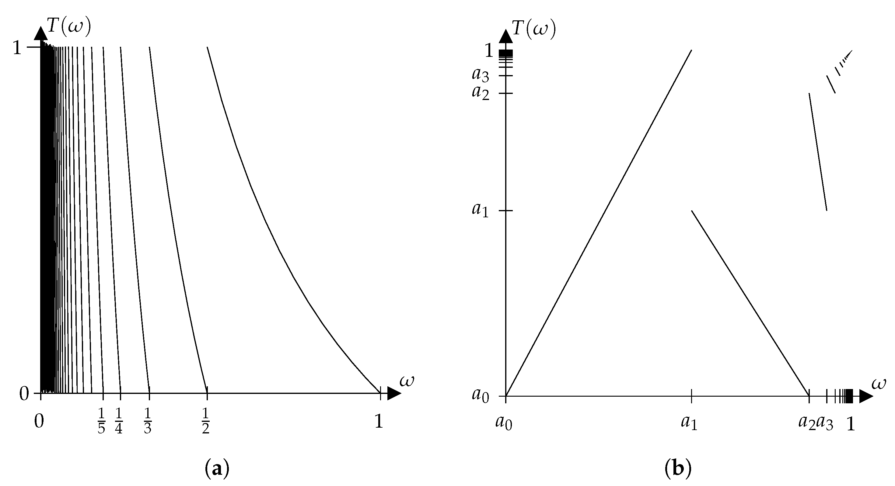
Example 1

(Gaussian map). The map $T:[0,1]\to [0,1]$ with

$$T\left(\omega \right)=\left\{\begin{array}{cc}1/\omega \mathrm{mod}1,\hfill & \mathrm{if}\omega >0,\hfill \\ 0,\hfill & \mathrm{if}\omega =0\hfill \end{array}\right.$$

is called a Gaussian map (see Figure 2a). This map is measure-preserving with regard to the measure μ, which is defined by $\mu \left(A\right)=\frac{1}{log2}{\int }_A\frac{1}{1+x}dx$ for all $A\in \mathcal{B}$ [11]. The partition $\mathcal{M}=\left\{\right[\frac{1}{n+1},\frac{1}{n}[\mid n\in \mathbb{N}\}\cup \left\{\left\{0\right\}\right\}$ of $[0,1]$ is a countably infinite partition into monotony intervals of T satisfying $H\left(\mathcal{M}\right)<\infty$. This map is countably piecewise monotone and ergodic. Thus, its Kolmogorov–Sinai entropy is equal to its permutation entropy.

Example 2.

Consider $\Omega =[0,1[$ and the Borel σ-algebra $\mathcal{B}$ on Ω. Set

$$\begin{array}{cc}\hfill S& :=\sum _{i=0}^{\infty }\frac{1}{(i+1){(log(i+1))}^2},\hfill \\ \hfill m_i& :=\frac{1}{S}·\frac{1}{(i+1){(log(i+1))}^2}\mathrm{for}i\in \mathbb{N},\hfill \\ \hfill a_0& :=0,\hfill \\ \hfill a_1& :=m_1,\hfill \\ \hfill a_i& :=1-\frac{m_{i+1}}{m_1}\mathrm{for}i\ge 2,\hfill \\ \hfill M_i& :=[a_{i-1},a_i]\mathrm{for}i\in \mathbb{N}.\hfill \end{array}$$

The map $T:\Omega \to \Omega$ is defined as piecewise linear on each set $M_i$ (see Figure 2b) by

$$T\left(\omega \right)=\left\{\begin{array}{cc}\frac{\omega }{m_1},\hfill & if\omega \in M_1,\hfill \\ a_{i-1}·\frac{a_i-\omega }{a_i-a_{i-1}}+a_{i-2}·\frac{\omega -a_{i-1}}{a_i-a_{i-1}},\hfill & if\omega \in M_{i}withi\in \mathbb{N}\backslash \left\{1\right\}.\hfill \end{array}\right.$$

Let λ be the one-dimensional Lebesgue measure. Define a measure μ on $(\Omega ,\mathcal{B})$ by

$$\mu \left(A\right):=\sum _{j=1}^{\infty }\frac{m_j·\lambda (A\cap M_j)}{\lambda \left(M_j\right)}$$

for all $A\in \mathcal{B}$.

One can verify that T is measure-preserving and ergodic with regard to μ. The partition $\mathcal{M}:={\left\{M_i\right\}}_{i\in \mathbb{N}}$ does satisfy (5) for $m=1$, but $H\left(\mathcal{M}\right)=\infty$ holds true. Therefore, Condition 1 does not hold true for $m=1$. However, one can show that Condition 1 holds true for $m=2$ and the partition ${\mathcal{M}}^{\prime }:=\{M_1,{\bigcup }_{m=2}^{\infty }{M}_i\}$, which implies that the Kolmogorov–Sinai entropy is equal to the permutation entropy of this map due to Theorem 4.

4. A Supplementary Aspect

To determine under what conditions the Kolmogorov–Sinai entropy and the upper or lower permutation entropies coincide remains an open problem in the general case, and in the simple one-dimensional case of maps not being (countably) piecewise monotone the relation of Kolmogorov–Sinai and upper and lower permutation entropies is not completely understood. There is not even known an example where the entropies differ. Finally, we shortly want to discuss a further approach for discussing the relationship of Kolmogorov–Sinai entropy and upper and lower permutation entropies.

In [12], it was shown that under (1) the Kolmogorov–Sinai entropy is equal to the permutation entropy if roughly speaking the information contents of ‘words’ of k ’successive’ ordinal patterns of large length n is not too far from the information contents of ordinal patterns of length $n+k-1$. We want to explain this for the simple one-dimensional case and $k=2$.

The ordinal pattern of some $(x_0,x_1,\dots ,x_n)$ contains all information on the order relation between the points $x_0,x_1,\dots ,x_n$. When considering the ‘overlapping’ ordinal patterns of $(x_0,x_1,\dots ,x_{n-1})$ and $(x_1,x_2,\dots ,x_n)$, one has the same information with one exception: The order relation between $x_0$ and $x_n$ is not known a priori. Looking at the related partitions, the missing information is quantified by the conditional entropy $H\left(OP\left(n+1\right)\right|OP\left(n\right)\vee T^{-1}\left(OP\left(n\right)\right))$. There is one situation reducing this missing information, namely that one of the $x_i;i=1,2,\dots ,n-1$ lies between $x_0$ and $x_n$. Then, the order relation between $x_0$ and $x_n$ is known by knowing the ordinal patterns of $(x_0,x_1,\dots ,x_{n-1})$ and $(x_1,x_2,\dots ,x_n)$. Therefore, the following set is of some special interest:

$$\begin{array}{cc}\hfill V_n:=& \left\{\omega \in \Omega \mid \omega \le T^n\left(\omega \right)\mathrm{and}{T}^s\left(\omega \right)\notin (\omega ,T^n\left(\omega \right))\mathrm{for}\mathrm{all}s\in \{1,2,\dots ,n-1\}\right\}\hfill \\ \hfill \cup & \left\{\omega \in \Omega \mid T^n\left(\omega \right)\le \omega \mathrm{and}{T}^s\left(\omega \right)\notin (T^n\left(\omega \right),\omega )\mathrm{for}\mathrm{all}s\in \{1,2,\dots ,n-1\}\right\}.\hfill \end{array}$$

(11)

The following is shown in Appendix A.5:

Lemma 1.

Let Ω be a subset of $\mathbb{R}$ and $\mathcal{A}=\mathcal{B}$ be the Borel σ-algebra on Ω. Then,

$$H\left(OP\left(n+1\right)|OP\left(n\right)\vee T^{-1}\left(OP\left(n\right)\right)\right)\le log\left(2\right)·\mu \left(V_n\right)$$

(12)

holds true for all $n\in \mathbb{N}$.

This indicates that analyzing the measure of $V_n$ as defined in (11) can be a useful approach to gain inside into the relationship between different kinds of entropies based on ordinal patterns. In particular, the behavior of $\mu \left(V_n\right)$ for $n\to \infty$ is of interest.

Lemma 2.

Let Ω be a subset of $\mathbb{R}$ and $\mathcal{A}=\mathcal{B}$ be the Borel σ-algebra on Ω. If T is ergodic, then

$$\underset{n\to \infty }{lim\; inf}\mu \left(V_n\right)=0$$

holds true, and, if (stronger) T is mixing, then

$$\underset{n\to \infty }{lim}\mu \left(V_n\right)=0$$

holds true.

The statement under the assumption of mixing has been shown in [5], and the proof in the ergodic case is given in Appendix A.5.

One can show that in the simple one-dimensional case the Kolmogorov–Sinai entropy is equal to the permutation entropy if

$$\sum _{n=1}^{\infty }H\left(OP\left(n+1\right)|OP\left(n\right)\vee T^{-1}\left(OP\left(n\right)\right)\right)<\infty$$

(13)

holds true. Using (12), this is the case when ${\sum }_{n=1}^{\infty }\mu \left(V_n\right)$ is finite, providing a fast decay of the $\mu \left(V_n\right)$. However, we have ${\sum }_{n=1}^{\infty }\mu \left(V_n\right)=\infty$ as stated in Theorem 5, which will be proved in Appendix A.6.

Theorem 5.

Let Ω be a subset of $\mathbb{R}$, $\mathcal{A}=\mathcal{B}$ be the Borel σ-algebra on Ω and T be aperiodic and ergodic. Then,

$$\sum _{n=1}^{\infty }\mu \left(V_n\right)=\infty$$

holds true.

Although formula ${\sum }_{n=1}^{\infty }\mu \left(V_n\right)<\infty$ is false, we cannot answer the question of whether or when (13) is valid. Possibly, an answer to this question, and a better understanding of the kind of decay of the $\mu \left(V_n\right)$, could be helpful in further investigating the relationship of Kolmogorov–Sinai entropy and upper and lower permutation entropies, at least in the simple one-dimensional ergodic case.

5. Conclusions

With Theorem 1, we have slightly generalized a statement given in [3] by removing a technical assumption and using more basic combinatorial arguments. The remaining assumption (1) on the random vector $\mathbf{X}$ cannot be weakened in general.

In Section 2.3, we have shown that the equality of the permutation entropy and the Kolmogorov–Sinai entropy implies the equality of conditional permutation entropy and Kolmogorov–Sinai entropies as well. We considered two different kinds of conditional permutation entropy, which have turned out to be equal in the cases considered in Section 2.3; it is however not clear whether these two kinds of conditional permutation entropy are equal in the general.

In Section 4, we have established some condition under which these two kinds of conditional entropy are equal, independently from of the equality between permutation and Kolmogorov–Sinai entropies. This condition is based on a concept introduced in [5] that was originally introduced as a tool for better understanding the relationship between permutation and Kolmogorov–Sinai entropies in a general setting. However, with Theorem 5, we have shown that this tool cannot directly be used to show the equality between permutation and Kolmogorov–Sinai entropies. It is an interesting question of whether and how a clever adaption and improvement of it can allow for new insights in the relationship between permutation and Kolmogorov–Sinai entropies.

In Section 3, we considered the simpler one-dimensional case. With Theorem 4, we have given two conditions under which the permutation entropy is a lower bound for the Kolmogorov–Sinai entropy. This theorem generalizes previous statements in [1] and slightly generalizes a statement in [10]. One of the conditions (Condition 2) holds true for a large class of dynamical systems, while, for the other one (Condition 1) to hold true, it is necessary that the system is in some sense ’order preserving’. It is still an unsolved and interesting question, whether Condition 1 can be weakened, especially since, to the best of our knowledge, there does not exist a counterexample to the equality of permutation entropy and Kolmogorov–Sinai entropies. Finding a generalization of Theorem 4 to a multidimensional setting is a further interesting question one could ask.

References

- Bandt, C.; Keller, G.; Pompe, B. Entropy of interval maps via permutations. Nonlinearity 2002, 15, 1595. [Google Scholar] [CrossRef]
- Amigó, J.M. The equality of Kolmogorov–Sinai entropy and metric permutation entropy generalized. Physica D 2012, 241, 789–793. [Google Scholar] [CrossRef]
- Antoniouk, A.; Keller, K.; Maksymenko, S. Kolmogorov–Sinai entropy via separation properties of order-generated σ-algebras. Discret. Cont. Dyn.-A 2014, 34, 1793. [Google Scholar]
- Fouda, E.; Koepf, W.; Jacquir, S. The ordinal Kolmogorov–Sinai entropy: A generalized approximation. Commun. Nonlinear Sci. 2017, 46, 103–115. [Google Scholar] [CrossRef]
- Unakafova, V.; Unakafov, A.; Keller, K. An approach to comparing Kolmogorov–Sinai and permutation entropy. Eur. Phys. J. Spec. Top. 2013, 222, 353–361. [Google Scholar] [CrossRef] [Green Version]
- Watt, S.; Politi, A. Permutation entropy revisited. Chaos Soliton Fract. 2019, 120, 95–99. [Google Scholar] [CrossRef] [Green Version]
- Bandt, C.; Pompe, B. Permutation Entropy: A Natural Complexity Measure for Time Series. Phys. Rev. Lett. 2002, 88, 174102. [Google Scholar] [CrossRef] [PubMed]
- Amigó, J.M.; Kennel, M.B.; Kocarev, L. The permutation entropy rate equals the metric entropy rate for ergodic information sources and ergodic dynamical systems. Physica D 2005, 210, 77–95. [Google Scholar] [CrossRef] [Green Version]
- Haruna, T.; Nakajima, K. Permutation complexity via duality between values and orderings. Physica D 2011, 240, 1370–1377. [Google Scholar] [CrossRef] [Green Version]
- Gutjahr, T.; Keller, K. Equality of Kolmogorov–Sinai and permutation entropy for one-dimensional maps consisting of countably many monotone parts. Discret. Cont. Dyn.-A 2019, 39, 4207. [Google Scholar] [CrossRef] [Green Version]
- Einsiedler, M.; Ward, T. Ergodic Theory: With a View Towards Number Theory; Graduate Texts in Mathematics; Springer: London, UK, 2010. [Google Scholar]
- Keller, K.; Unakafov, A.M.; Unakafova, V.A. On the relation of KS entropy and permutation entropy. Physica D 2012, 241, 1477–1481. [Google Scholar] [CrossRef] [Green Version]
- Walters, P. An Introduction to Ergodic Theory; Graduate Texts in Mathematics; Springer: New York, NY, USA, 2000. [Google Scholar]
- Rokhlin, V.A. On the fundamental ideas of measure theory. Am. Math. Soc. Transl. 1952, 71, 55. [Google Scholar]
- Heinemann, S.; Schmitt, O. Rokhlin’s Lemma for Non-invertible Maps. Dyn. Syst. Appl. 2001, 2, 201–213. [Google Scholar]
- Halmos, P.R. Extension of Measures. In Measure Theory; Springer: New York, NY, USA, 1950; pp. 49–72. [Google Scholar]
Figure 1.
Abstract visualization of all 24 possible ordinal patterns of length 4.
Figure 2.
(a) Graph of the Gaussian map. (b) Graph of the map given in Example 2.
© 2020 by the authors. Licensee MDPI, Basel, Switzerland. This article is an open access article distributed under the terms and conditions of the Creative Commons Attribution (CC BY) license (http://creativecommons.org/licenses/by/4.0/).
Share and Cite
MDPI and ACS Style
Gutjahr, T.; Keller, K. Ordinal Pattern Based Entropies and the Kolmogorov–Sinai Entropy: An Update. Entropy 2020, 22, 63. https://0-doi-org.brum.beds.ac.uk/10.3390/e22010063
AMA Style
Gutjahr T, Keller K. Ordinal Pattern Based Entropies and the Kolmogorov–Sinai Entropy: An Update. Entropy. 2020; 22(1):63. https://0-doi-org.brum.beds.ac.uk/10.3390/e22010063
Chicago/Turabian StyleGutjahr, Tim, and Karsten Keller. 2020. "Ordinal Pattern Based Entropies and the Kolmogorov–Sinai Entropy: An Update" Entropy 22, no. 1: 63. https://0-doi-org.brum.beds.ac.uk/10.3390/e22010063
Note that from the first issue of 2016, this journal uses article numbers instead of page numbers. See further details here.