Monitoring Volatility Change for Time Series Based on Support Vector Regression


Department of Statistics, Seoul National University, Seoul 08826, Korea
*
Author to whom correspondence should be addressed.
Entropy 2020, 22(11), 1312; https://0-doi-org.brum.beds.ac.uk/10.3390/e22111312
Submission received: 21 October 2020
/
Revised: 13 November 2020
/
Accepted: 13 November 2020
/
Published: 17 November 2020
(This article belongs to the Special Issue Theory and Applications of Information Theoretic Machine Learning)
Abstract
:This paper considers monitoring an anomaly from sequentially observed time series with heteroscedastic conditional volatilities based on the cumulative sum (CUSUM) method combined with support vector regression (SVR). The proposed online monitoring process is designed to detect a significant change in volatility of financial time series. The tuning parameters are optimally chosen using particle swarm optimization (PSO). We conduct Monte Carlo simulation experiments to illustrate the validity of the proposed method. A real data analysis with the S&P 500 index, Korea Composite Stock Price Index (KOSPI), and the stock price of Microsoft Corporation is presented to demonstrate the versatility of our model.
1. Introduction
In this paper, we study the cumulative sum (CUSUM) monitoring procedure to sequentially detect a significant change in time series with conditional volatilities. Since [1,2], the CUSUM method has been an acclaimed tool to detect an anomaly among observations in statistical process control (SPC). In SPC, a control chart is a primary component that graphically describes the behavior of sequentially observed time series. For examples of SPC, see [3] for control charts, [4] for the analysis of complex environmental time series, and [5] for backcasting-forecasting time series. In particular, the CUSUM chart is one of the most frequently adopted methods among various fields of SPC. For an overview of SPC, we refer to [6]. In general, the performance of control charts is measured with average run length (ARL). However, instead of the conventional control charts, some authors, such as [7], alternatively took the approach of controlling type I errors in probability instead of controlling ARL to deal with the monitoring process in autoregressive time series. This design of the sequential monitoring method has merit in its ability to attain a lower false alarm rate, as seen in [8], who took a similar approach to dealing with generalized autoregressive conditional heteroscedastic (GARCH) time series. For more references as to the monitoring process in time series, see [9]. Here, inspired by the previous studies, we aim to hybridize the CUSUM monitoring scheme with support vector regression (SVR) for GARCH-type time series.
Support vector machine (SVM) is one of the most popular nonparametric learning methods used predominantly for classification and regression [10]. In particular, compared with traditional model-based methods, the support vector regression (SVR) is more advantageous to approximating the nonlinearity of the underlying dynamic structure of datasets. Refer to [11,12,13,14,15], and the papers cited therein. Moreover, SVR is structured to exploit the quadratic programming optimization problem, and to implement the structural risk minimization principle [16]. This facilitates SVR to be an estimation scheme that optimally minimizes the empirical risk while being relatively parsimonious [17]. This further enables the SVR to perform adequately for variously sized datasets, including the case where its size is relatively small. Refs. [18,19] recently used the SVR with a hybridization of the CUSUM method to detect a change point in SVR-autoregressive and moving average (ARMA) and SVR-GARCH models. Therein, the residual-based CUSUM test has been adopted by referring to the previous studies of [20,21,22]. See [23] for a general overview of the change point detection problem using CUSUM methods. In the same spirit, here we also take the approach of the CUSUM of squares test, rather than the score vector-based CUSUM test used in [7,8], as the former largely outperforms the latter in terms of stability and power, as seen in the empirical study of [21]; above all, the latter is only available for the model-based CUSUM test. As pointed out in the precedent works of [18,19], the role of the accurately computed residuals is substantially important, and thereby, so is the precise prediction of the used SVR method. As the optimal choice of tuning parameters matters to a significant degree as well, we consider adopting particle swarm optimization (PSO) [24] for the purpose of tuning parameter optimization. For a theoretical background, we refer to [25,26,27]. See also the survey papers of [28,29,30]. These are population-based algorithms and have been widely used to obtain optimal tuning parameters in SVR. Therefore, we evaluate the performance of the proposed SVR-GARCH-based CUSUM monitoring method equipped with the PSO through Monte Carlo experiments.
The rest of this paper is organized as follows. Section 2 introduces the CUSUM monitoring and explains its fundamental principle and application to GARCH-type time series. Section 3 describes SVR and PSO in general, then elaborates on the monitoring process for SVR-GARCH models in more detail. Section 4 presents Monte Carlo simulations conducted to evaluate the performance of the proposed method. Section 5 performs a real data analysis using the S&P 500 index, KOSPI, and the stock returns of Microsoft Corporation datasets. Finally, Section 6 provides concluding remarks.
2. CUSUM Monitoring Procedure
In this section, we introduce our monitoring process starting from the independent and identically distributed (iid) sample case. Let us consider the problem of monitoring an anomaly in the variance from a stream of observations of mean zero up to time n. Under the null hypothesis of no anomalies, we assume that are iid with unit variance over time . Namely, we test
For this task, we first define
for each , where , which is assumed to be known. Ref. [7] considered the monitoring process based on:
and later [8] additionally considered the monitoring process based on:
In this study, however, we consider another monitoring process based on
with
We employ the test statistic because it combines the strength of and , which detect well the decrease and increase of variance, respectively. Note that if has a positive shift, say, from 1 to with , at some point , for would tend to have larger values due to the shift, which, however, is not true for , indicating that would be able to detect the shift well while would not do so; by contrast, if has a negative shift, would be able to detect the shift well while would not do so. Additionally, is preferable over in (3) as the latter tends to detect well a change that occurs in the middle of time series.
Using Donsker’s invariance principle [31] and the fact that in distribution for any standard Brownian motion , as described in [7], we have that as ,
where denotes a convergence in distribution, and implies the distribution functions of random variables X and Y being equivalent. Furthermore, by the continuous mapping theorem, in (4) satisfies
Then, the null hypothesis is rejected if is larger than a constant c, which is determined asymptotically as the number satisfying for any significance . In practice, we can obtain the critical value c empirically using Monte Carlo simulations. For example, when . Thus, an anomaly is signaled at k when for some .
This monitoring process can be extended to the GARCH(1,1) model [32]:
with satisfying and . This model is widely used to model financial time series with high volatilities as it captures well the volatility clustering phenomenon. For its properties and characteristics and various GARCH variants, see [19,33], and the papers cited therein. Here, the monitoring process can be constructed based on residuals with with some initial values and when the true parameters are known in advance from past experience. However, when they are unknown, which is a prevalent phenomenon in practice, we instead construct the CUSUM test with residuals with , where are estimators of obtained from a given training sample. Then, we employ the following:
where are the same as in (2) and (5), , with in (1) replaced by , and and are the sample mean and variance of the residuals obtained from the training sample, respectively. We reject the null hypothesis if for the aforementioned critical value . Theoretically, the limiting distribution of is anticipated to be the same as the one in (6) when certain conditions are fulfilled, namely satisfies as (e.g., for some ) and is a (-consistent) Gaussian quasi-maximum likelihood estimator (QMLE) as in [33], the proof of which is rather standard and omitted for brevity. The monitoring process of the nonlinear time series via SVR is provided in Section 3.3 below.
3. Monitoring Procedure via SVR-GARCH Model
3.1. Support Vector Regression
Support vector regression (SVR) is a nonparametric function estimating method, which is a branch of the support vector machine that originated from [34] as a classification tool. Here, SVR is utilized to conduct CUSUM tests, as it effectively incorporates circumstances where the underlying structure of the conditional variance presented in (7) is unknown, and possibly nonlinear. Its details will be elaborated in Section 3.3 below.
In SVR, we seek to find a function of the form:
where x denotes a vector of explanatory variables, w and b are regression parameters to be estimated, and is an implicit kernel operator that satisfies for some pre-defined kernel function K.
To obtain the estimates of the regression parameters, we then formulate the problem where we can exploit its structure to employ a quadratic programming method [17]:
where denote slack variables, denotes a penalty term, and is a tuning parameter that determines the level of tolerance regarding the error. Note that C and are user-defined tuning parameters of the model.
By the duality of the Karush–Khun–Tucker condition, we obtain the following optimization problem with respect to the Lagrange multipliers and as dual variables [16]:
Consequently, the solutions of the optimization problem (10) constructs the estimate of f as follows:
where can be obtained with various approaches. See [17] or [35] for references.
The tuning parameters of our SVR-GARCH model consist of , and , as we utilize the Gaussian kernel function
Moreover, as the tuning parameters are user-defined, it must either be selected prior to employing the SVR, or be optimized. Here, we utilize the PSO to select the set of tuning parameters. The procedure of the PSO algorithm is elucidated in more detail in the next section.
3.2. Particle Swarm Optimization
PSO is one of the widely acclaimed meta-heuristic methodologies and is extensively adopted when optimizing tuning parameters in various machine learning techniques. Initially proposed by [24], its ability of optimization in nonlinear and nonconvex problems is inspired by the movement of organisms in bird flocks or animal herds. Here, we refer to [30] to describe the procedure.
Given a suitable objective function, a standard PSO algorithm aims to optimize a d-dimensional parameter x in the following search space:
for some , . A particle j at time t, denoted by a d-dimensional vector in with
is considered as a candidate of the set of optimal solutions. Moreover, a swarm at time t is defined as . Each particle j has its own d-dimensional velocity vector at time t, denoted by for , where
is a velocity space with and being the lower and upper bound of each velocity element, respectively [36]. Furthermore, the best optimal solution is defined as:
where denotes the trajectory of the particle j until time t.
Then, the global best optimal solution of the trajectory of all particles until time t is defined as . In each generation at time , where is a prescribed maximum generation time, the j-th particle in swarm is updated as follows:
where are acceleration factors in and are random variables generated from a uniform distribution . In addition, is an inertia term at time t, which is calculated as follows:
where and are predefined lower and upper bounds of the inertia values, respectively. Ref. [30] recently proved that the optimal solution obtained from the PSO algorithm converges to the global optimum with probability 1 under regularity conditions.
The process of the aforementioned PSO algorithm is condensed in Algorithm 1 below.
| Algorithm 1 Standard PSO algorithm |
| 1: procedure PSO() |
| 2: |
| 3: |
| 4: while do |
| 5: ; |
| 6: |
| 7: for do |
| 8: update ; |
| 9: ; |
| 10: update |
| 11: end for |
| 12: update |
| 13: end while |
| 14: end procedure |
3.3. Monitoring Nonlinear Time Series via SVR
We extend the monitoring process introduced in Section 2 to embrace nonlinear GARCH models with the following form:
where g is an unknown, possibly nonlinear, function to be estimated, is the conditional volatility, and are iid errors with zero mean and unit variance. To obtain the residuals that formulate the test statistic (8) of the monitoring process, we estimate g by with a training sample . For the estimation procedure, we utilize the SVR and then adopt the notion of the retrospective test described in [19].
For estimating via SVR, we first divide the training sample into two distinct samples, say and , then regard the latter as the validation set. Subsequently, we replace with its proxy , as is unknown in practice. The authors of [14] employed the moving average method with a window size as below:
for , where are some sensible initial values. Although its validity is advocated when in [19], we alternatively consider the exponentially-weighted moving average (EWMA) estimator
where is a tuning parameter, which we set to 0.94 in our study, and is some initial value. This alteration improves both the stability and the performance of the model, as portrayed in Section 4.
Moreover, to further enhance the stability of the estimation process of , we log-transform the response variable of (11), then take the exponential to obtain . To elaborate, we recursively obtain through as follows:
Given and a space of tuning parameters , we then employ the PSO algorithm to obtain an optimal set of tuning parameters by evaluating the mean absolute error (MAE):
where and are obtained with a validation time series. Ultimately, the finalized is obtained by utilizing all the training samples and .
The test set of length n emerges sequentially in practice, denoted by . Then, utilizing , we yield the residuals
where is obtained recursively through (12). Afterwards, upon observing , the monitoring procedure is conducted by computing the CUSUM test statistic as in (8), and we declare it out of control when it exceeds the prescribed critical value under the nominal level .
Remark 1.
In our proposed monitoring procedure, we use the theoretically obtained critical value c, as illustrated by its notable performance in Section 4. However, if m is not large enough relative to n, there is a chance that the monitoring procedure might be undermined by the parameter estimation. In this case, one may be able to obtain c empirically through a wild bootstrap approach with the following steps [21]:
- 1.
- Estimate with from training sample ;
- 2.
- Estimate recursively with and some initial values and ;
- 3.
- Generate iid standard normal random variables , , , and construct a bootstrap sample ;
- 4.
- Based on , , estimate with , and calculate the bootstrapped residuals with obtained recursively by ;
- 5.
- Based on these residuals, construct the monitoring process , , , similarly to in (8) with analogously defined to ;
- 6.
- Finally, the critical value c is determined as the upper quantile of for .
The critical value c can be obtained via a bootstrap method similar to that for the GARCH(1,1) model in (7). In this case, we use . Based on the obtained bootstrap sample , applying the SVR method again, we can get the conditional volatility estimates , where are proxies obtained from ’s. Then, the bootstrapped residuals are obtained as . The critical value is obtained from these similarly to Steps (5) and (6) addressed above. Instead of , alternatively one might be able to consider using to obtain the residuals .
4. Simulation Experiments
We assess the proposed SVR-GARCH monitoring process to measure the performance when the time series is simulated from linear or nonlinear variants of GARCH models, such as GARCH, asymmetric GARCH (AGARCH), GJR-GARCH, and Box–Cox transformed threshold GARCH (BCTT-GARCH), specified as follows:
where the orders are fixed as 1 and the errors are iid. are random variables.
In implementation, we generate a time series of length m from each of the above models and fit the SVR-GARCH model to it as presented in Section 3. In this procedure, we utilize the first time series as a training set, and the rest as a validation set, where denotes the largest integer not exceeding x. Subsequently, to create the circumstance, where the dataset for monitoring (testing sample) is observed sequentially, we initially design the underlying parametric model with a change located at point . With this model, we generate a single observation of time series, obtain the residuals with the trained SVR-GARCH model, and then compute the test statistic. We terminate this monitoring process either if the test statistics are larger than the critical value c, or the accumulated number of observations reaches the prescribed length of n. To obtain the sizes and powers empirically, we iterate the procedure 1000 times at the significance level of . The empirical sizes and powers are calculated as the ratio of the rejections of the null hypothesis out of the 1000 repetitions.
Upon the construction of the null hypothesis, we consider the following settings:
- GARCH(1,1):
- AGARCH(1,1):
- GJR-GARCH(1,1):
- BCTT-GARCH(1,1): .
We inspect the cases of and , where is used, i.e., for , respectively, and count the number of false alarms and anomaly detections when the underlying model experiences a change at diverse locations, namely at the observation of the monitoring time series for . For each set of experiments, we employ the PSO search algorithm for optimizing tuning parameters.
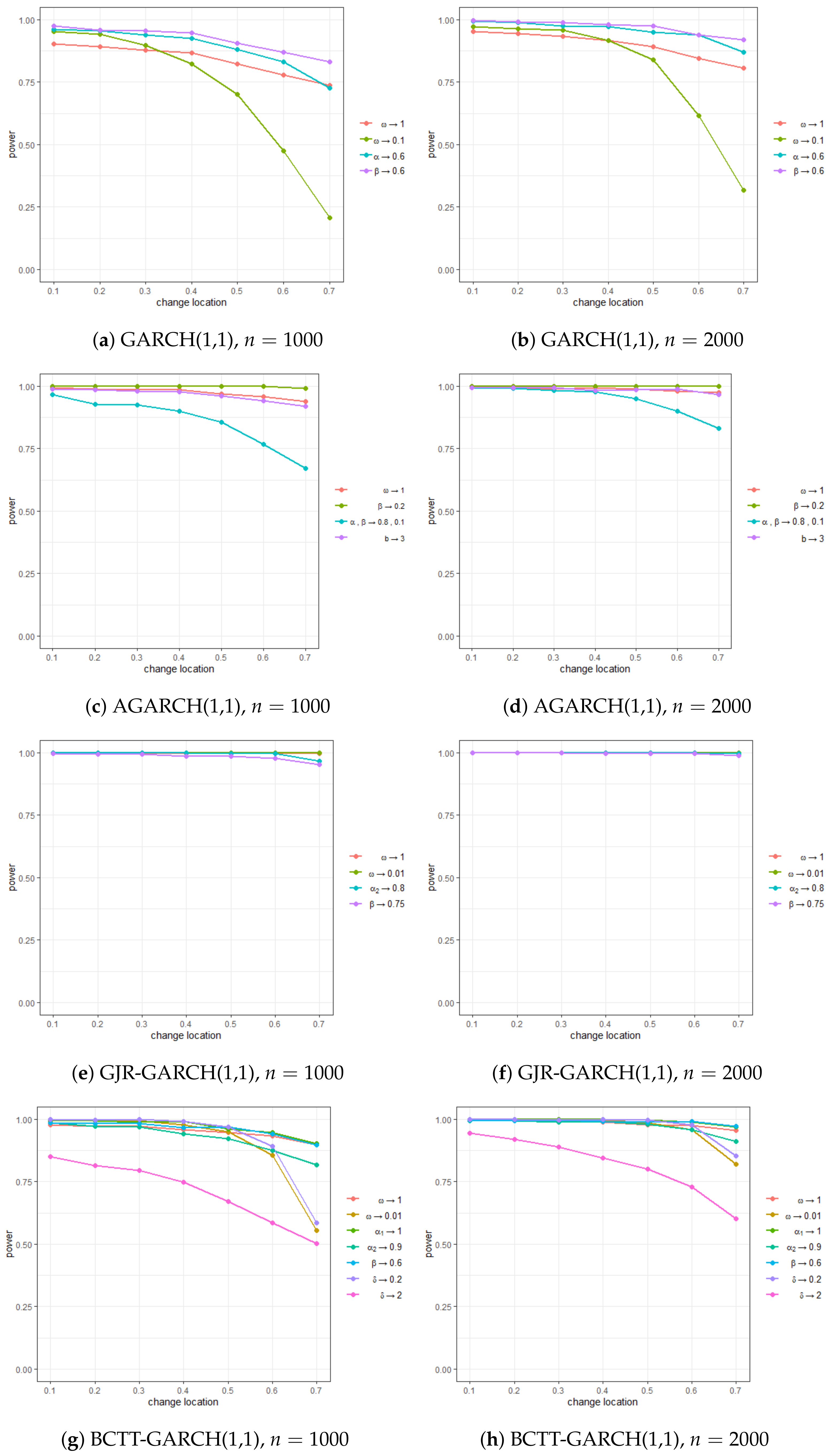
Table 1 and Figure 1 encapsulate the empirical sizes and powers for the above four cases. In a nutshell, all four models’ empirical sizes show a tendency to stabilize around . Additionally, their empirical powers approached 1 in a vast majority of the experiments, exhibiting a remarkable ability to detect changes across the experiments. In particular, as anticipated, the power became more significant as the decreases. Nevertheless, even if the location of the change was towards the end of the observation (i.e., a larger ), its detection ability was still not heavily deteriorated. This entails that the performance of our monitoring process is not much affected by the location of change.
The result for the AGARCH model, presented in Figure 1c,d, is particularly more prominent. Despite the model being systematically unstable because of being close to 1, empirical sizes and powers appeared to be highly reliable even at a relatively small sample size of . This robustly confirms the validity of our proposed method. Overall, our findings show that the proposed monitoring process is highly applicable to datasets with high volatilities, such as the daily returns of financial time series.
5. Real Data Analysis
In this section, we demonstrate the real-world applicability of our proposed SVR-GARCH monitoring scheme with three financial time series: the S&P500 Composite Index (2 January 1991∼31 December 2003), the Korea Composite Stock Price Index (KOSPI) (2 July 2012∼29 September 2020), and the stock price of Microsoft Corporation (1 July 2009∼30 September 2020), obtainable from the websites Yahoo Finance and Investing.com. Moreover, the log returns, defined as , are utilized throughout the analysis, and are denoted by “S&P500”, “KOSPI”, and “Microsoft”.
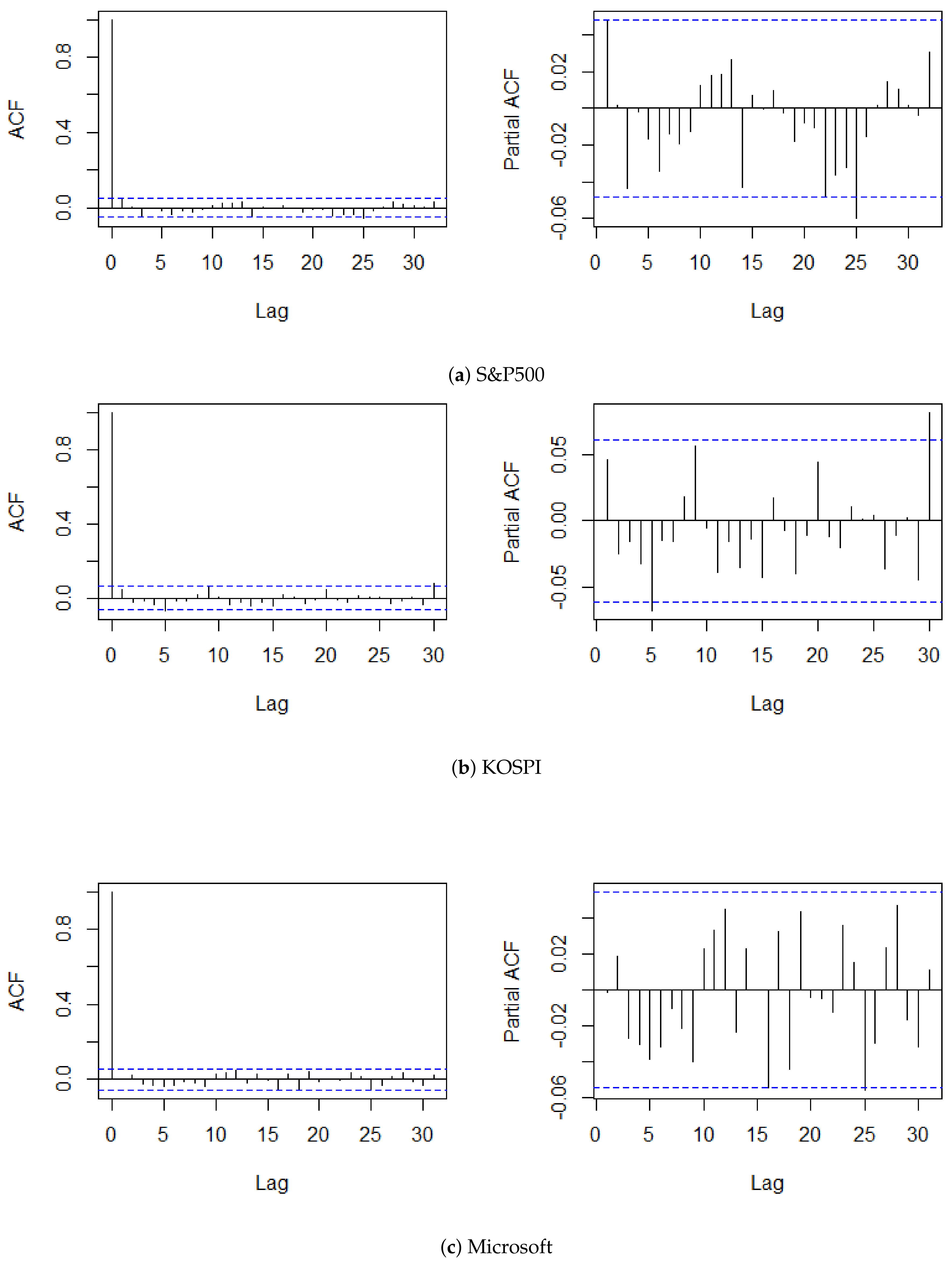
The procedure of this analysis is categorized into four steps. We first divided the time series of log returns into two chunks, and assigned the former as the training set of size m. To reflect the situation of monitoring, setting the maximum number of observations to , we regarded the latter time series being observed sequentially. We then overviewed the general behavior of the given time series with its summary statistics, autocorrelation functions (ACFs), and partial ACFs (PACFs). Table 2 and Figure 2 reveal the basic characteristics of the datasets and plots of the ACFs and PACFs up to lag 25, respectively. The characteristics of KOSPI is similar to those of the standard normal distribution, in terms of skewness and excess kurtosis. By contrast, the excess kurtosis of S&P500 and Microsoft drifted from that of a standard normal distribution, and was moderately skewed, compared to KOSPI. Moreover, the ACFs and PACFs of all three time series did not suggest significant autocorrelations, which entails the stationarity of the datasets. Additionally, fitting the SVR-GARCH model of Lee et al. (2020b) to examine an existence of change within the training time series, we applyed their retrospective CUSUM test to the training set. Then, the result exhibited that it did not exceed the critical value of 1.3397, which consolidated the absence of change within the training set at the significance level of .
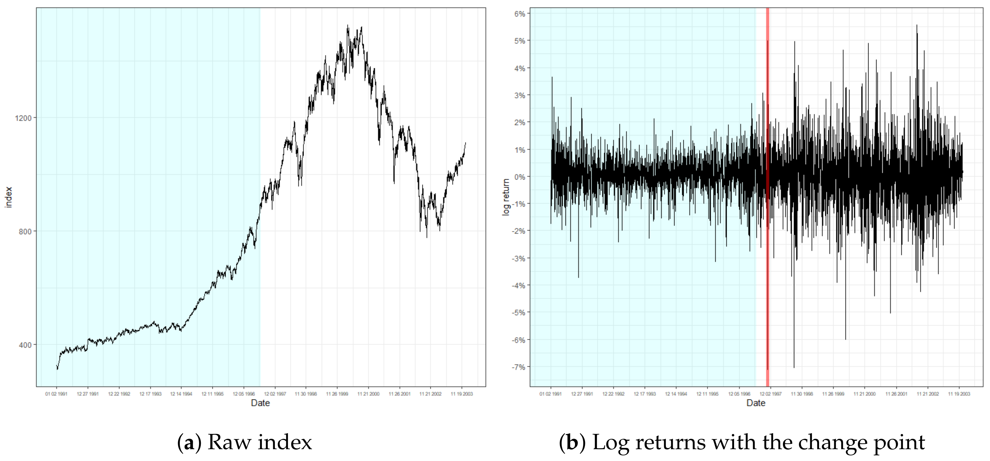
Figure 3, Figure 4 and Figure 5 present the result of the monitoring procedure and the identified location of change in conditional volatility. The change of volatility for S&P500 appeared to occur on 28 October 1997. Notably, our model promptly responded to the event that occurred on the day prior, where log returns fluctuated by more than 7%. Additionally, we can observe the increase of volatility posterior to the detected location. Indeed, the detected location is around the period of the Asian financial crisis of 1997, and specifically on the exact date when the South Korean won plummeted massively to its new low. This instantaneous response after an abrupt change of volatility strengthens the validity of our monitoring process.
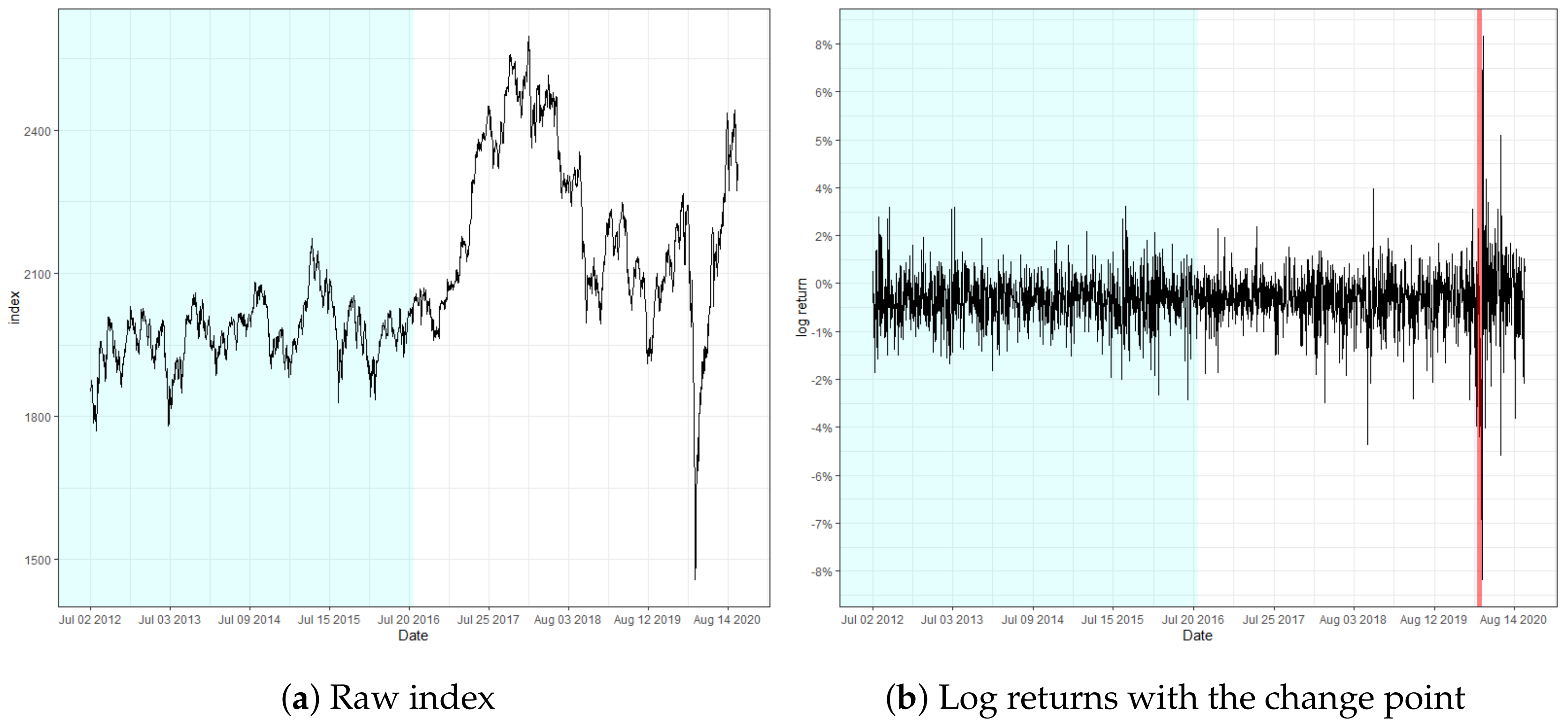
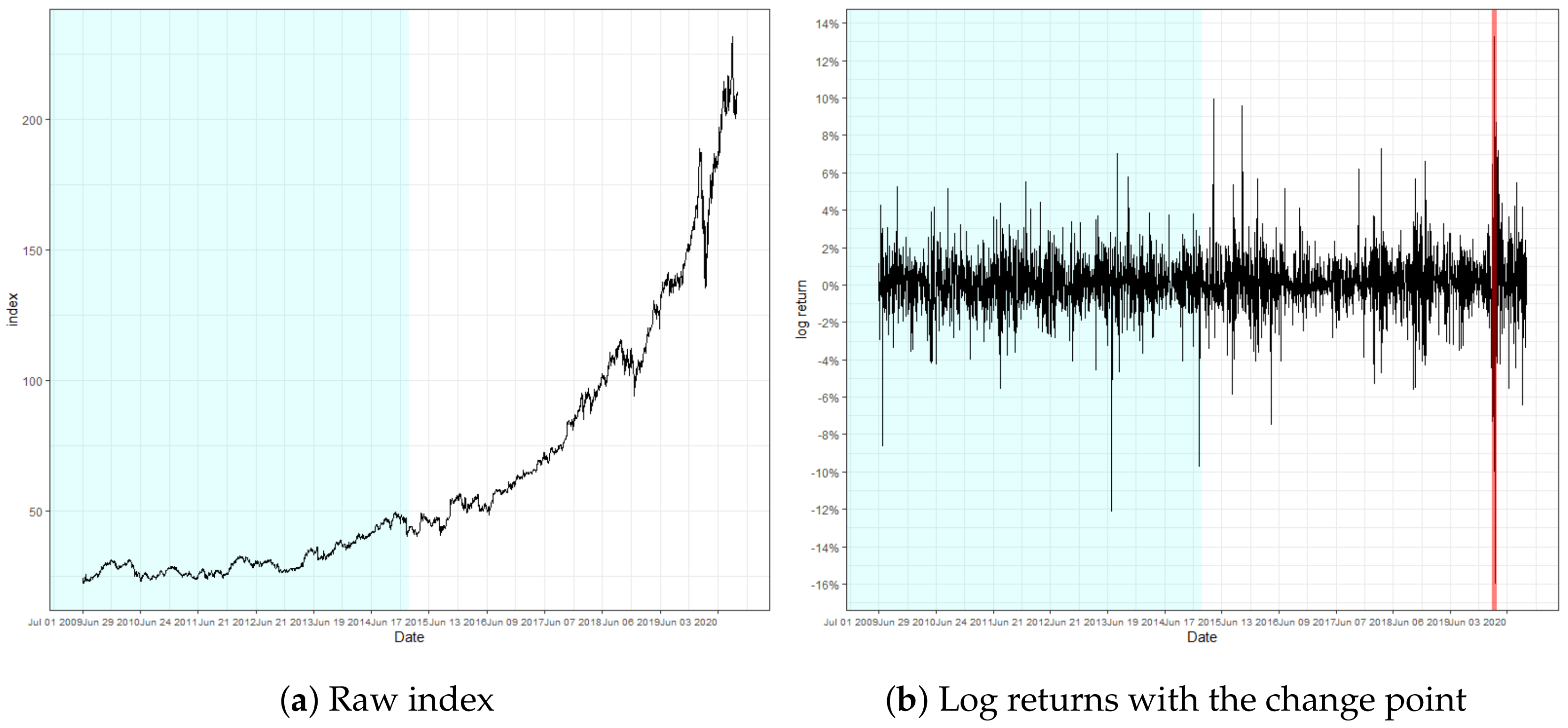
The locations of change regarding KOSPI and Microsoft were observed on 11 March and 13 March 2020, respectively. Notice that the detected location of change is close to the predetermined n. These findings particularly implicate that the detection ability of our monitoring process is not impaired, even if the volatility change is located near the end. In addition, the change point in KOSPI predates the major spread of the global pandemic outbreak by a few days, where the log-returns are observed to fluctuate abruptly, exceeding 8%. In fact, the recognized locations of change regarding KOSPI and Microsoft are around the period of the stock market crash resulting from the pandemic, which still currently affects the global financial market to a certain extent. This result illuminates the potential of our monitoring scheme to identify a signal change prior to the change in the underlying structure of the model and to serve as a solution to the necessity of prompt detection of structural changes throughout various fields of research.
6. Concluding Remarks
In this study, we considered a novel monitoring process for detecting a significant change of conditional volatilities in time series. For this task, we proposed a procedure based on a CUSUM test with a new test statistic, and utilized the SVR-GARCH model to calculate the residuals so as to construct the monitoring process, wherein the PSO is employed to obtain an optimal set of tuning parameters. Our simulation study demonstrated the adequacy of the proposed monitoring process for various linear and nonlinear GARCH-type time series. A real data analysis of three financial time series, namely S&P500, KOSPI, and Microsoft, was conducted to affirm the practicability of our model in various real-world circumstances. Our proposed model can be adopted in a classical SPC, where one controls ARL directly rather than the Type I error. This could be empirically achieved using the bootstrap method, as stated in Section 3.3. As the necessity for control charts with their usage tailored to various circumstances is still increasing, we leave the issue as our future research project.
Author Contributions
Conceptualization, S.L.; methodology, S.L.; software, C.K.K. and D.K.; validation, S.L. and C.K.K.; formal analysis, C.K.K. and D.K.; investigation, S.Y. and C.K.K.; resources, S.Y.; data curation, C.K.K.; writing—original draft preparation, S.L. and C.K.K.; writing—review and editing, S.L. and C.K.K.; visualization, C.K.K.; supervision, S.L.; project administration, S.L.; funding acquisition, S.L. All authors have read and agreed to the published version of the manuscript.
Funding
This research was supported by the Basic Science Research Program through the National Research Foundation of Korea funded by the Ministry of Science, ICT and future Planning (grant 2018R1A2A2A05019433).
Acknowledgments
We thank the three anonymous referees for their careful reading and valuable comments that improved the quality of the paper.
Conflicts of Interest
The authors declare no conflict of interest. The funding sponsors had no role in the design of the study; in the collection, analyses, or interpretation of data; in the writing of the manuscript, and in the decision to publish the results.
Abbreviations
The following abbreviations are used in this manuscript:
| CUSUM | cumulative sum |
| SPC | statistical process control |
| ARL | average run length |
| ARMA | autoregressive and moving average |
| ARCH | autoregressive conditionally heteroskedasticity |
| GARCH | generalized autoregressive conditionally heteroskedasticity |
| SVR | support vector regression |
| SVM | support vector machine |
| PSO | particle swarm optimization |
| iid | independent and identically distributed |
| MAE | mean absolute error |
| EWMA | exponentially weighted moving average |
| AGARCH | asymmetric GARCH |
| GJR-GARCH | Glosten, Jagannathan and Runkle-GARCH |
| BCTT-GARCH | Box-Cox transformed threshold GARCH |
| ARMA | autoregressive and moving average |
| QMLE | quasi-maximum likelihood estimator |
| KOSPI | Korea Composite Stock Price Index |
| ACF | autocorrelation function |
| PACF | partial ACF |
References
- Page, E.S. Continuous inspection schemes. Biometrika 1954, 41, 100–115. [Google Scholar] [CrossRef]
- Page, E.S. A test for a change in a parameter occurring at an unknown point. Biometrika 1955, 42, 523–527. [Google Scholar] [CrossRef]
- Wu, Z.; Jiao, J.; Yang, M.; Liu, Y.; Wang, Z. An enhanced adaptive CUSUM control chart. IIE Trans. 2009, 41, 642–653. [Google Scholar] [CrossRef]
- Regier, P.; Briceño, H.; Boyer, J.N. Analyzing and comparing complex environmental time series using a cumulative sums approach. MethodsX 2019, 6, 779–787. [Google Scholar] [CrossRef]
- Contreras-Reyes, J.E.; Idrovo-Aguirre, B.J. Backcasting and forecasting time series using detrended cross-correlation analysis. Phys. A Stat. Mech. Appl. 2020, 560, 125109. [Google Scholar] [CrossRef]
- Montgomery, D.C. Statistical Quality Control; Wiley Global Education: Hoboken, NJ, USA, 2012. [Google Scholar]
- Gombay, E.; Serban, D. Monitoring parameter change in AR (p) time series models. J. Multivar. Anal. 2009, 100, 715–725. [Google Scholar] [CrossRef]
- Huh, J.; Oh, H.; Lee, S. Monitoring parameter change for time series models with conditional heteroscedasticity. Econ. Lett. 2017, 152, 66–70. [Google Scholar] [CrossRef]
- Na, O.; Lee, Y.; Lee, S. Monitoring parameter change in time series models. Stat. Methods Appl. 2011, 20, 171–199. [Google Scholar] [CrossRef]
- Vapnik, V. Statistical Learning Theory; John Wiley and Sons: New York, NY, USA, 1998. [Google Scholar]
- Fernandez-Rodriguez, F.; Gonzalez-Martel, C.; Sosvilla-Rivero, S. On the profitability of technical trading rules based on artificial neural networks: Evidence from the Madrid stock market. Econ. Lett. 2000, 69, 89–94. [Google Scholar] [CrossRef]
- Cao, L.; Tay, F. Financial forecasting using support vector machines. Neural Comput. Appl. 2001, 10, 184–192. [Google Scholar] [CrossRef]
- Pérez-Cruz, F.; Afonso-Rodriguez, J.; Giner, J. Estimating GARCH models using SVM. Quant. Financ. 2003, 3, 163–172. [Google Scholar] [CrossRef]
- Chen, S.; Härdle, W.K.; Jeong, K. Forecasting volatility with support vector machine-based GARCH model. J. Forecast. 2010, 29, 406–433. [Google Scholar] [CrossRef]
- Bezerra, P.; Albuquerque, P. Volatility forecasting via SVR–GARCH with mixture of Gaussian kernels. Comput. Manag. Sci. 2017, 14, 179–196. [Google Scholar] [CrossRef]
- Vapnik, V.N. The Nature Of Statistical Learning Theory; Springer: New York, NY, USA, 2000. [Google Scholar]
- Smola, A.; Schölkopf, B. A tutorial on support vector regression. Stat. Comput. 2004, 14, 199–222. [Google Scholar] [CrossRef] [Green Version]
- Lee, S.; Lee, S.; Moon, M. Hybrid change point detection for time series via support vector regression and CUSUM method. Appl. Soft Comput. 2020, 89, 106101. [Google Scholar] [CrossRef]
- Lee, S.; Kim, C.; Lee, S. Hybrid CUSUM change point test for time series with time-varying volatilities based on support vector regression. Entropy 2020, 22, 578. [Google Scholar] [CrossRef]
- Lee, S.; Tokutsu, Y.; Maekawa, K. The cusum test for parameter change in regression models with ARCH errors. J. Jpn. Stat. Soc. 2004, 34, 173–188. [Google Scholar] [CrossRef] [Green Version]
- Oh, H.; Lee, S. Modified residual CUSUM test for location-scale time series models with heteroscedasticity. Ann. Inst. Stat. Math. 2019, 71, 1059–1091. [Google Scholar] [CrossRef]
- Lee, S. Location and scale-based CUSUM test with application to autoregressive models. J. Stat. Comput. Simul. 2020, 90, 2309–2328. [Google Scholar] [CrossRef]
- Lee, S.; Ha, J.; Na, O.; Na, S. The CUSUM test for parameter change in time series models. Scand. J. Stat. 2003, 30, 781–796. [Google Scholar] [CrossRef]
- Kennedy, J.; Eberhart, R. Particle swarm optimization. In Proceedings of the ICNN’95-International Conference on Neural Networks, Perth, Australia, 27 November–1 December 1995; IEEE: Piscataway, NJ, USA, 1995; Volume 4, pp. 1942–1948. [Google Scholar]
- Ozcan, E.; Mohan, C.K. Analysis of a simple particle swarm optimization system. Intell. Eng. Syst. Through Artif. Neural Netw. 1998, 8, 253–258. [Google Scholar]
- Trelea, I.C. The particle swarm optimization algorithm: Convergence analysis and parameter selection. Inf. Process. Lett. 2003, 85, 317–325. [Google Scholar] [CrossRef]
- Yasuda, K.; Ide, A.; Iwasaki, N. Adaptive particle swarm optimization. In SMC’03 Conference Proceedings, Proceedings of the 2003 IEEE International Conference on Systems, Man and Cybernetics, Washington, DC, USA, 8 October 2003; IEEE: Piscataway, NJ, USA, 2003; Volume 2, pp. 1554–1559. [Google Scholar]
- Zhang, Y.; Wang, S.; Ji, G. A comprehensive survey on particle swarm optimization algorithm and its applications. Math. Probl. Eng. 2015, 2015, 1–38. [Google Scholar] [CrossRef] [Green Version]
- Wang, D.; Tan, D.; Liu, L. Particle swarm optimization algorithm: An overview. Soft Comput. 2018, 22, 387–408. [Google Scholar] [CrossRef]
- Qian, W.; Li, M. Convergence analysis of standard particle swarm optimization algorithm and its improvement. Soft Comput. 2018, 22, 4047–4070. [Google Scholar] [CrossRef]
- Billingsley, P. Convergence of Probability Measure; Wiley: New York, NY, USA, 1968. [Google Scholar]
- Bollerslev, T. Generalized autoregressive conditional heteroskedasticity. J. Econom. 1986, 31, 307–327. [Google Scholar] [CrossRef] [Green Version]
- Francq, C.; Zakoian, J.M. GARCH Models: Structure, Statistical Inference and Financial Applications; John Wiley & Sons: New York, NY, USA, 2019. [Google Scholar]
- Cortes, C.; Vapnik, V. Support-vector networks. Mach. Learn. 1995, 20, 273–297. [Google Scholar] [CrossRef]
- Abe, S. Support Vector Machines for Pattern Classification; Springer: New York, NY, USA, 2005; Volume 2. [Google Scholar]
- Marini, F.; Walczak, B. Particle swarm optimization (PSO). A tutorial. Chemom. Intell. Lab. Syst. 2015, 149, 153–165. [Google Scholar] [CrossRef]
Figure 1.
Plots of empirical power of the SVR-GARCH monitoring procedure.

Figure 2.
Plot of ACF and PACF up to lag 25 of log-returns.

Figure 3.
Raw index and its log returns of S&P500.

Figure 4.
Raw index and its log returns of KOSPI.

Figure 5.
Raw index and its log returns of Microsoft.


Table 1.
Empirical size and power of the SVR-GARCH monitoring procedure for the GARCH(1,1), AGARCH(1,1), GJR-GARCH(1,1), and BCTT-GARCH(1,1) models.
Table 1.
Empirical size and power of the SVR-GARCH monitoring procedure for the GARCH(1,1), AGARCH(1,1), GJR-GARCH(1,1), and BCTT-GARCH(1,1) models.
| 4-17 | ||||||||||||||||
|---|---|---|---|---|---|---|---|---|---|---|---|---|---|---|---|---|
| Change location | ||||||||||||||||
| GARCH(1,1) | size | 0.038 | 0.045 | |||||||||||||
| power | 0.903 | 0.893 | 0.879 | 0.867 | 0.824 | 0.778 | 0.737 | 0.953 | 0.945 | 0.934 | 0.916 | 0.893 | 0.845 | 0.805 | ||
| 0.954 | 0.942 | 0.898 | 0.824 | 0.701 | 0.475 | 0.206 | 0.971 | 0.963 | 0.959 | 0.916 | 0.840 | 0.616 | 0.317 | |||
| 0.961 | 0.955 | 0.940 | 0.924 | 0.882 | 0.830 | 0.726 | 0.995 | 0.990 | 0.976 | 0.973 | 0.951 | 0.939 | 0.870 | |||
| 0.974 | 0.958 | 0.955 | 0.946 | 0.907 | 0.871 | 0.832 | 0.996 | 0.992 | 0.988 | 0.981 | 0.975 | 0.940 | 0.920 | |||
| AGARCH(1,1) | size | 0.039 | 0.037 | |||||||||||||
| power | 0.993 | 0.989 | 0.987 | 0.985 | 0.968 | 0.959 | 0.939 | 0.996 | 0.997 | 0.988 | 0.995 | 0.989 | 0.980 | 0.975 | ||
| 1.000 | 1.000 | 1.000 | 1.000 | 1.000 | 1.000 | 0.992 | 1.000 | 1.000 | 1.000 | 1.000 | 1.000 | 1.000 | 1.000 | |||
| 0.967 | 0.927 | 0.924 | 0.900 | 0.856 | 0.767 | 0.672 | 0.995 | 0.992 | 0.983 | 0.978 | 0.950 | 0.899 | 0.832 | |||
| 0.989 | 0.986 | 0.981 | 0.978 | 0.962 | 0.943 | 0.920 | 0.994 | 0.995 | 0.994 | 0.984 | 0.987 | 0.988 | 0.966 | |||
| GJR-GARCH(1,1) | size | 0.042 | 0.033 | |||||||||||||
| power | 1.000 | 0.999 | 1.000 | 0.998 | 0.999 | 0.998 | 0.996 | 1.000 | 1.000 | 1.000 | 1.000 | 0.999 | 1.000 | 0.999 | ||
| 1.000 | 1.000 | 1.000 | 1.000 | 1.000 | 1.000 | 1.000 | 1.000 | 1.000 | 1.000 | 1.000 | 1.000 | 1.000 | 1.000 | |||
| 1.000 | 1.000 | 0.999 | 0.999 | 0.998 | 0.997 | 0.967 | 1.000 | 1.000 | 1.000 | 1.000 | 0.999 | 1.000 | 0.998 | |||
| 0.996 | 0.993 | 0.994 | 0.986 | 0.986 | 0.977 | 0.954 | 1.000 | 1.000 | 1.000 | 0.998 | 0.998 | 0.997 | 0.989 | |||
| BCTT-GARCH(1,1) | size | 0.048 | 0.039 | |||||||||||||
| power | 0.978 | 0.973 | 0.973 | 0.957 | 0.948 | 0.934 | 0.897 | 0.997 | 0.996 | 0.993 | 0.989 | 0.979 | 0.975 | 0.955 | ||
| 0.995 | 0.995 | 0.993 | 0.978 | 0.951 | 0.855 | 0.556 | 0.999 | 0.997 | 0.997 | 0.997 | 0.987 | 0.958 | 0.819 | |||
| 0.997 | 0.995 | 0.988 | 0.992 | 0.962 | 0.947 | 0.903 | 1.000 | 0.999 | 1.000 | 1.000 | 0.996 | 0.989 | 0.968 | |||
| 0.987 | 0.971 | 0.968 | 0.941 | 0.921 | 0.875 | 0.817 | 0.995 | 0.993 | 0.988 | 0.992 | 0.980 | 0.958 | 0.911 | |||
| 0.986 | 0.983 | 0.984 | 0.967 | 0.970 | 0.941 | 0.897 | 0.998 | 0.994 | 0.997 | 0.992 | 0.990 | 0.992 | 0.972 | |||
| 0.999 | 0.998 | 0.999 | 0.992 | 0.969 | 0.891 | 0.585 | 0.999 | 0.999 | 0.998 | 0.999 | 0.996 | 0.978 | 0.854 | |||
| 0.850 | 0.814 | 0.795 | 0.749 | 0.671 | 0.585 | 0.502 | 0.945 | 0.919 | 0.890 | 0.846 | 0.800 | 0.728 | 0.602 | |||
Table 2.
Summary statistics and the results of the preliminary retrospective test of the training set, and the result of the monitoring test regarding S&P500, KOSPI, and Microsoft.
Table 2.
Summary statistics and the results of the preliminary retrospective test of the training set, and the result of the monitoring test regarding S&P500, KOSPI, and Microsoft.
| S&P500 | KOSPI | Microsoft | ||
|---|---|---|---|---|
| Summary statistics (training set) | Observations | 1640 | 1016 | 1417 |
| Mean | 0.0604 | 0.0096 | 0.0428 | |
| Standard deviation | 0.6931 | 0.7728 | 1.4408 | |
| Minimum | −3.7272 | −3.1429 | −12.1033 | |
| Median | 0.0352 | 0.0070 | 0.03145 | |
| Maximum | 3.6642 | 2.9124 | 7.0330 | |
| Skewness | −0.1064 | −0.0264 | −0.6141 | |
| Excess kurtosis | 2.2428 | 1.3848 | 6.8293 | |
| Retrospective test (training set) | Test statistic | 0.8069 | 1.2876 | 0.5897 |
| Monitoring test | Location | 97/10/28 | 20/03/11 | 20/03/13 |
Publisher’s Note: MDPI stays neutral with regard to jurisdictional claims in published maps and institutional affiliations. |
© 2020 by the authors. Licensee MDPI, Basel, Switzerland. This article is an open access article distributed under the terms and conditions of the Creative Commons Attribution (CC BY) license (http://creativecommons.org/licenses/by/4.0/).
Share and Cite
MDPI and ACS Style
Lee, S.; Kim, C.K.; Kim, D. Monitoring Volatility Change for Time Series Based on Support Vector Regression. Entropy 2020, 22, 1312. https://0-doi-org.brum.beds.ac.uk/10.3390/e22111312
AMA Style
Lee S, Kim CK, Kim D. Monitoring Volatility Change for Time Series Based on Support Vector Regression. Entropy. 2020; 22(11):1312. https://0-doi-org.brum.beds.ac.uk/10.3390/e22111312
Chicago/Turabian StyleLee, Sangyeol, Chang Kyeom Kim, and Dongwuk Kim. 2020. "Monitoring Volatility Change for Time Series Based on Support Vector Regression" Entropy 22, no. 11: 1312. https://0-doi-org.brum.beds.ac.uk/10.3390/e22111312
Note that from the first issue of 2016, this journal uses article numbers instead of page numbers. See further details here.