Relative Distribution Entropy Loss Function in CNN Image Retrieval


1
College of Computer Science and Technology, Jilin University, Changchun 130012, China
2
Key Laboratory of Symbolic Computation and Knowledge Engineering of Ministry of Education, Jilin University, Changchun 130012, China
3
School of Mechanical Science and Engineering, Jilin University, Changchun 130025, China
4
College of Software, Jilin University, Changchun 130012, China
5
College of Communication Engineering, Jilin University, Changchun 130012, China
*
Author to whom correspondence should be addressed.
Entropy 2020, 22(3), 321; https://0-doi-org.brum.beds.ac.uk/10.3390/e22030321
Submission received: 31 January 2020
/
Revised: 5 March 2020
/
Accepted: 9 March 2020
/
Published: 11 March 2020
(This article belongs to the Special Issue Information Transfer in Multilayer/Deep Architectures)
Abstract
:Convolutional neural networks (CNN) is the most mainstream solution in the field of image retrieval. Deep metric learning is introduced into the field of image retrieval, focusing on the construction of pair-based loss function. However, most pair-based loss functions of metric learning merely take common vector similarity (such as Euclidean distance) of the final image descriptors into consideration, while neglecting other distribution characters of these descriptors. In this work, we propose relative distribution entropy (RDE) to describe the internal distribution attributes of image descriptors. We combine relative distribution entropy with the Euclidean distance to obtain the relative distribution entropy weighted distance (RDE-distance). Moreover, the RDE-distance is fused with the contrastive loss and triplet loss to build the relative distributed entropy loss functions. The experimental results demonstrate that our method attains the state-of-the-art performance on most image retrieval benchmarks.
1. Introduction
In recent years, the newly proposed image retrieval algorithms based on convolutional neural networks [1,2,3,4,5] (CNN) have greatly improved the accuracy and efficiency. This has been the mainstream direction of academic research of image retrieval. In the beginning, CNN could only be applied to image classification tasks [6,7,8]. However, image classification is different from the image retrieval. Krizhevsky [9] flexibly applied a convolutional neural network to image retrieval. AlexNet [9] is designed for image classification and retrieval. Subsequently, Noh [10] proposed a Local Feature descriptor, called DELF (Deep Local Feature), which is suitable for large-scale image retrieval. A large number of studies have illustrated that the output features of the convolutional layer of the neural network have excellent discrimination and scalability. More recently, image retrieval algorithms based on convolutional neural networks emerged one after another. These methods are mainly summarized into three categories: fine-tuned networks, pre-trained networks, and hybrid networks. Among them, hybrid networks are less efficient in image retrieval tasks, and pre-trained networks are widely used. The fine-tuned network initializes the network architecture through the pre-trained image classification model and then adjusts the parameters according to different retrieval tasks. The fine-tuned network usually optimizes the network parameters by training the network architecture of metric learning. Metric learning aims to learn an embedding space, where the embedded vectors of positive samples are encouraged to be closer, while negative samples are pushed apart from each other [11,12,13]. Recently, a lot of deep metric learning methods have been based on pairs of samples such as contrastive loss [14], triplet loss [15], quadruplet loss [16], lifted structured loss [17], N-pairs loss [18], binomial deviance loss [19], histogram loss [20], angular loss [21], distance weighted margin-based loss [22], and hierarchical triplet loss (HTL) [23]. Most of the above-mentioned loss functions take common vector similarity (such as Euclidean distance) as the final image descriptor into consideration. However, it is not accurate enough to measure the similarity between features only by Euclidean distance, which lacks the difference in the internal spatial distribution [24] of the image pair. As illustrated in Figure 1, each rectangle represents a feature descriptor obtained after the convolution of the neural network. The value of Euclidean distance between descriptors for different images may be the equal or small, but the spatial distribution of every descriptor may be greatly different. In the information processing field, entropy [25] is an effective measurement to reflect the distribution information. Relative entropy [26,27,28] is a measure of the distance between two random distributions, which is equivalent to the difference of information entropy between two distributions. Inspired by this, we introduce the idea of relative entropy into image retrieval.
To solve the key problem mentioned above, we propose relative distribution entropy (RDE) to describe the distribution attributes of image descriptors. We combine the relative distribution entropy with the Euclidean distance [29] to build the relative distribution entropy weighted distance (RDE-distance). We fuse the RDE-distance into the contrastive loss and triplet loss to obtain the relative distributed entropy contrastive loss and the relative distributed entropy triplet loss. We call them the relative distributed entropy loss functions. To be more specific, we make three contributions, as follows:
Firstly, we propose a loss function modified by relative distribution entropy, called the relative distribution entropy loss function. Furthermore, the relative distribution entropy loss function contains the following two aspects: (1) Euclidean distance between the descriptors. (2) The differences in internal distribution state between descriptors. The core idea of the algorithm is illustrated in Figure 2. We combine the Euclidean distance with the relative distribution entropy to obtain the relative distribution entropy weighted distance (RDE-distance), which increases the discrimination between the image pair. We replace the Euclidean distance in the original contrastive loss and triplet loss with the relative distribution entropy weighted distance (RDE-distance) to obtain the relative distribution entropy loss function.
Thirdly, we employ the fine-tuned network [30] to perform our experiments on different datasets to verify the effectiveness of our proposed method.
The organization of this work is as follows. Section 2 introduces the related work. Section 3 mainly introduces our proposed relative distribution entropy loss function. Specific experimental results and analyses will be presented in Section 4. Section 5 is a summary of the contributions and methods of this paper.
2. Related Work
2.1. Deep Metric Learning
Deep metric learning (DML) has become one of the most interesting research areas in machine learning. Metric learning aims to learn an embedding space. In this space, images are converted into embedding vectors. The distance between embedding vectors of positive samples is small, and the distance between embedding vectors of negative samples is large [11,12,13]. Now, deep metric learning has played a vital role in many areas, such as face recognition [32], pedestrian recognition [33], fine-grained retrieval [34], image retrieval [35], target tracking [36], and multimedia retrieval [37]. We will summarize the recent emergence of metric learning methods in the next section. Here, we introduce deep metric learning into image retrieval. Deep metric learning aims to learn a discriminative feature embedding for input image . In other words, is the descriptor of the image. Formally, we define the Euclidean distance between two descriptors as .
2.1.1. Contrastive Loss
The siamese network [14] is a typical pair-based method. Its embedding is obtained through contrastive loss. The purpose of contrastive loss is to reduce the Euclidean distance between positive samples and increase the Euclidean distance between negative samples. The equation of the contrastive loss function is illustrated in (1).
if the sample is a positive sample, and if the sample is a negative sample. is the margin. This keeps negative distances above a certain threshold.
2.1.2. Triplet Loss
However, the above models only focus on the similarity of intra-class of the samples. To solve this problem, the triplet loss function [15] is proposed. Each triplet comprises a positive sample and a negative sample sharing the query. Triplet loss aims to learn an embedding space. In this space, the distance between the query and the negative sample is greater than the distance between the query and the positive sample. The triplet loss function is illustrated in (2).
Here, represents the Euclidean distance between the descriptors of the positive sample and the query. Similarly, represents the Euclidean distance between the descriptors of the negative sample and the query. is the violate margin that requires that the negative distances to be larger than the positive distances.
2.1.3. N-pair Loss
Triplet loss function only compares one negative sample and ignores the negative samples of other classes during the learning stage. As a result, the embedding vector of the query can only be promoted to maintain a large distance between the selected negative samples, but it cannot guarantee to maintain a large distance between the embedding vector and other non-selected negative samples.
N-pair loss [18] has improved the above problems. Unlike triplet loss function, N-pair loss considers the relationship between query samples and other negative samples of different classes within a mini-batch. The equation of the N-pair loss function is illustrated in (3).
Each training tuple of N-pair loss is composed of samples: . is the positive sample. are the negative samples.
2.1.4. Lifted Structured Loss
The existing triplet loss methods cannot take full advantage of mini-batch SGD training. Lifted structured loss calculates loss [17] based on all positive and negative sample pairs in the training set (mini-batch). The lifted structured loss function is illustrated in Equation (4).
where is the set of positive samples in the training set, and is the set of positive samples in the training set. is the violate margin.
Although these loss functions calculate the distance of descriptors between images, they neglect the difference in internal distribution between the image pair. In this work, we propose a new loss function, which is called the relative distribution entropy loss function. We use the relative distribution entropy to reflect the difference in the descriptor distribution, and add this difference to the loss function. In this way, the new loss function can combine the Euclidean distance with the internal relative difference in the distribution state between the descriptors of the image pair.
2.2. Application of Spatial Information in Image Retrieval
The performance of image retrieval has been greatly improved in recent years through the use of deep feature representations. However, most existing methods aim to retrieve images that are visually similar or semantically relevant to the query, without considering the spatial information. Before that, some researchers attempted to add spatial information into image retrieval algorithms to improve retrieval performance. Mehmood [38] proposed adding a local region and a global histogram to the BoW algorithm and combining them as the final descriptor. Krapac [39] used the BoW descriptor to encode the spatial part of the image, which improved the performance of the image classification. Koniusz [40] used spatial coordinate coding to represent and simplify the spatial pyramid to provide more compact image features. Sanchezet [41] added the spatial position information of features into the descriptor, which overcame the change in the proportion of retrieved objects and the change in the local area of the image. Liu [42] introduced the concept of spatial distribution entropy and combined it with the VLAD algorithm. These methods have fully introduced the spatial information into the image retrieval algorithm, and great effects are obtained. However, these methods all aimed at the improvement of traditional image descriptors. In this work, we attempt to add spatial information to the descriptor by optimizing the loss function of a deep convolutional network.
2.3. Pooling and Normalization
The feature map generated by the deep retrieval framework reflects the color, texture, shape, and other characteristics of the image. Since the convolutional neural network needs to be integrated into a multi-dimensional feature descriptor before retrieval, the feature map of the convolutional layer needs to be further processed. It is required that the processed result retains the main features of the image while reducing the parameters and calculations of the next layer. Babenko [43] proposed the mean-pooling method, which sums the pixel values of the feature map to obtain an N-dimensional feature vector. Razavian [44] used max-pooling or mean-pooling on the feature descriptors and the result reduced MAC [44] descriptors in dimension with a series of normalization and PCA [45] whitening operations. Finally, the region feature vectors are summed to obtain a single image representation. In this work, we used the generalized mean-pooling [30]. We used to represent the input to the pooling layer and to represent the pooling layer output. The mentioned pooling can be expressed as follows:
Max pooling (MAC vector):
Average pooling (SPoC vector [43]):
Generalized mean pooling (GeM [30]):
where is the number of feature maps, means the channel of features and is the number of feature values in the -th channel feature map. The descriptor finally consists of a single value per feature map. is the pooling parameter, which can be manually set or learned. The superscript of is the pooling method. represent the max pooling, average pooling and generalized mean pooling, respectively.
The max-pooling and mean-pooling are special cases of generalized mean-pooling. When, it is the mean-pooling. On the contrary, when it is positive infinity, it is the max-pooling. Generalized mean-pooling with parameters can better adapt to the network and improve retrieval performance.
In this work, we use normalization to balance the effect of the range of pixel values as follows:
where represents a vector, represents the norm of the vector, and represents the value of the dimension on the vector.
2.4. Whitening
In large-scale image retrieval applications, high-dimensional global images typically require the use of PCA to reduce the dimensions of features for the next step. Jegou and Chum [45] studied the influence of PCA on the BoW and VLAD descriptor representations, and highlighted the use of multiple visual dictionaries for dimensionality reduction, thereby reducing the information loss of the dimensionality reduction process. In this work, whitening is used as a post-processing step. In this paper, the method of whitening is the linear discriminant projection proposed by Mikolajczyk and Matas [31].
The processing steps are divided into two parts. In the first part, the intra-class image feature vector is whitened. The whitening part is the reciprocal of the square root of the intra-class image pair (matched image pair) covariance matrix .
where and are the descriptors of the image after pooling, represents the image matched pair, and represents the covariance matrix of the matched image pair.
In the second part, the inter-class image feature is rotated. The rotating part is the eigenvector of the covariance matrix between inter-class image pair (the non-matched image pair)
where and are the descriptors of the image after pooling, represents the non-matched image pair, and represents the covariance matrix of the non-matched image pair.
Then, we apply the projection to , where is the mean GeM [30] vector to perform centering.
3. Method Overview
3.1. Calculation of Relative Distribution Entropy
We firstly introduce the concept of relative distribution entropy. Relative distribution entropy can better represent the distribution difference between two descriptors of image samples. The relative distribution entropy is derived from the relative entropy. Relative entropy can be computed as follows:
and are the two probability distributions on the random variable . From this, we can get the equation of relative distribution entropy (RDE).
where represent the images. represents the descriptor of image . It is a normalized vector. is the relative distribution entropy of two images. In this work, we use histograms to describe the distribution of image descriptors. is the number of bins, and is an adjustable parameter. is the probability distribution in the bin. The equation for is the same as for. is the dimension of descriptors.
3.2. Relative Distribution Entropy Loss Function
From the above, we introduce the calculation of relative distributed entropy. Next, we show how to add the relative distribution entropy into the loss function. We add the relative distribution entropy to contrastive loss [14] and triplet loss [15] to build relative distribution entropy loss functions.
Firstly, we introduce the fusion process of contrastive loss and relative distribution entropy. The equation of the contrastive loss function is shown in (14).
where represents the Euclidean distance between the descriptors of the query and the sample . if the sample is a positive sample, and if the sample is a negative sample. is the margin.
Then, we add the relative distribution entropy to to get the :
where is the weighting parameter of the relative distribution entropy. As illustrated in Equation (16), we get the new distance metric. We call it the relative distribution entropy weighted distance (RDE-distance). We substitute into (14) to get the new contrastive loss function, as is shown in Equation (17):
Similarly, we introduce the fusion process of triplet loss and relative distribution entropy. The equation of the contrastive loss function is shown in (18).
is the Euclidean distance between the descriptors of the positive sample and the query. Similarly, is the Euclidean distance between the descriptors of the negative sample and the query.
Then, we add the relative distribution entropy to to get the.
We substitute the new Euclidean distances into Equation (18) and get the new triplet loss.
3.3. Network Architecture for Relative Distribution Entropy Loss Function
3.3.1. CNN Network Architecture
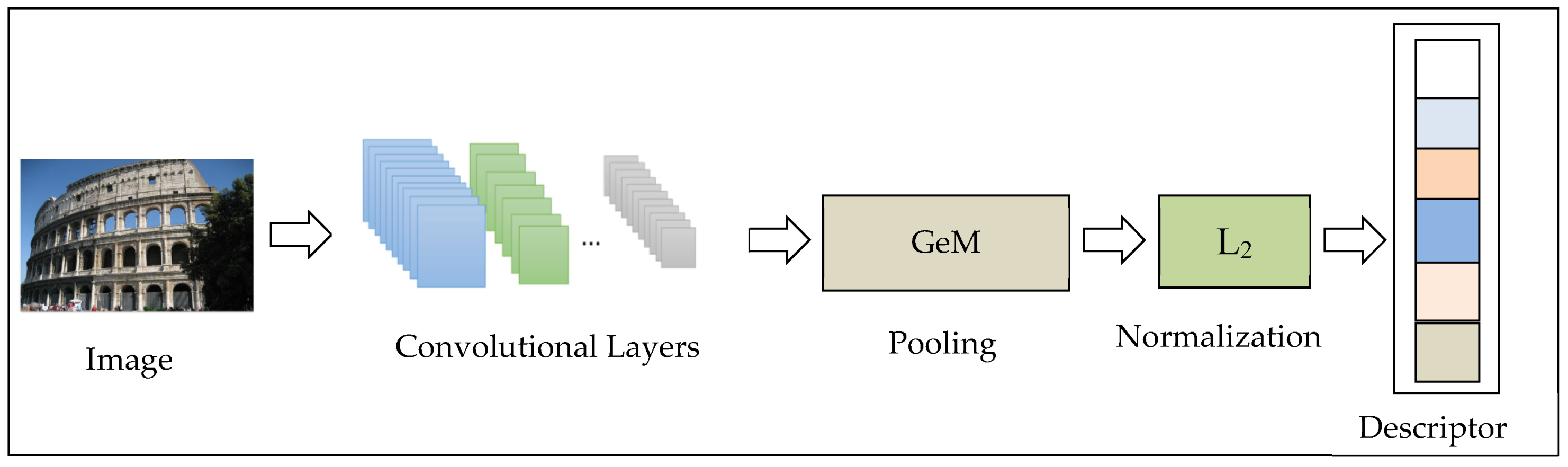
We construct a CNN neural network to obtain the descriptor of the image. We only use the convolutional layers, discarding the fully connected layer. Convolution layers can extract features of images. The feature map obtained by the convolution layer is vectorized by the GeM pooling operation [30]. If the whitening operation is performed, the whitening is processed following the pooling layer. Whitening can reduce the correlation between features, and it can make the features share the same variance (covariance matrix is 1), which can greatly improve the image retrieval performance. Here, we use the whitening [31] method. The last step is the normalization operation. The purpose of normalization is to make the preprocessed data limited to a certain range (such as [0,1] or [−1,1]), thereby eliminating the adverse effects caused by the singular sample data. The network architecture is pre-trained in ImageNet [46] network architecture.
Furthermore, we adopt network architectures such as ResNet [47] and AlexNet [9], and these two networks are also pre-trained on ImageNet [46].
The CNN network architecture is shown in Figure 3.
3.3.2. Architecture of Training
4. Experiments and Evaluation
In this section, we discuss the implementation details of training and testing. Also, we analyze the experimental results and compare them with previous work.
4.1. Training Datasets
In this work, experimental training data are distilled from Retrieval-SFM-120K [48], which contains 7.4 million images. After clustering [49], we get about 20,000 images as the query seed. The structure-from-motion (SfM) algorithm constructs 1474 3D models from the training datasets. We removed the duplications and retained 713 of them, which contained more than 163,000 different images.
There are 91,642 training images in the dataset, and 98 cluster images that are the same or almost the same as the test dataset. Through the minimum hash and spatial verification methods mentioned in the clustering process, about 20,000 images are selected as query images, 18,1697 pairs of positive images and 551 training clusters, including more than 163,000 clusters [50] from the original dataset. The dataset contains all images from the Oxford 5k [51] and Paris 6k [52] datasets.
4.2. Training Configurations
In the experiments, we use the Pytorch deep learning framework to train the deep network model. We use ResNet [47], VGG [53] and AlexNet [9], which are all pre-trained on ImageNet [46].
In the experiment of relative distribution entropy contrastive loss, ResNet [47] and VGG [53] are trained using Adam learning strategy [54], while AlexNet [9] is trained using SGD. Our initial learning rate for Adam is , and the margin for ResNet and VGG are 0.95 and 0.9. We use an initial learning rate equal to for SGD, and the margin for AlexNet is 0.75.
In the experiment of triplet loss, we also use ResNet [47], VGG [53], and AlexNet [9] to initialize the network. They are trained using the Adam learning strategy [54]. Our initial learning rate for Adam is . The margin for ResNet and VGG are 0.5, and the margin for AlexNet is 0.3. The size of the training image is not more than 362 * 362 while maintaining the aspect ratio of the original image.
The experimental environment is an intel(R) i7-8700 processor, GPU with 12GB of memory, NVIDIA(R) 2080Ti graphics card, driver version 419.**. Operating system is Ubuntu 18.04 LTS, PyTorch version v1.0.0, CUDA version 10.0, CUDNN version 7.5. The time spent in each training cycle trained on our method on VGG, ResNet, and AlexNet is 0.48, 0.72, and 0.22 hours, respectively. During the testing phase, testing VGG, ResNet, and AlexNet networks takes 620, 990, and 277 seconds, respectively. There are subtle differences between different test sets. With the same computing power, the training time of our method is almost the same as that of other methods [30].
4.3. Datasets and Evaluation of Image Retrieval
We conduct our testing experiments on the following benchmark datasets frequently. Herein, we give the details of these datasets.
Oxford5k [51] is a widely used landmark dataset consisting of 5062 building images from the Flickr dataset. It contains 11 famous landmarks in the Oxford area, and each landmark building has 55 query images.
Paris6k [52] contains 6392 images and is also one of the widely used datasets in the field of image retrieval. It collects many landmark buildings in Paris, and most of these images are from tourists. Similar to the Oxford 5k dataset, it also has 55 query images.
In addition, we use 100k interference images to fuse with the Oxford5k and Paris6k datasets to obtain Oxford105k [51] and Paris106k [52].
In the experiments, we use mean average precision (mAP) to measure the performance of image retrieval.
4.4. Results and Analysis
4.4.1. The Adjustment Process of Hyperparameter
In this experiment, two hyperparameters and are adjusted to obtain best performance. is the weight of the relative distribution entropy. As mentioned in Section 3.2, when fusing the Euclidean distance with RDE, the weight will affect the ratio of Euclidean distance and relative distribution entropy to the finally generated RDE-distance. As mentioned in Section 3.1, is the total bin amount in the histogram during the calculation of RDE. will affect the degree of differentiation of internal spatial distribution differences between two descriptors. However, a large also increases the computational burden. The ability of RDE-distance to distinguish between two descriptors is determined by two factors and . The values of these two hyperparameters have a great impact on our experimental results. During our experiments, we adjust them to get the best performance. We use AlexNet and VGG networks for tuning and the GeM pooling [30]. The partially representative results are shown in Table 1.
Here, we take some representative results. In the relative distribution entropy contrastive loss, we take the value of within 0.5–1, and the results show that the performance is the best when . Additionally, we take the value of within 10–100. When the value of is large (), the effect of adding relative distribution entropy is not obvious. After a large number of experiments, we can make the following conclusions. When and , our performance achieve the best results on Oxford5k and Pairs6k. The performance achieves 88.00% and 88.12% on VGG. On AlexNet, the performance achieves 68.22% and 80.07%. Therefore, we set to 30 and to 0.9 in ResNet and VGG as our final hyperparameters.
4.4.2. Comparison of MAC, SPoC, and GeM
In this section, we combine the relative distribution entropy contrastive loss function with the current most advanced pooling methods, GeM [30], MAC [44] and SPoc [43], for end-to-end training. In this experiment, we use the AlexNet for training. The experimental results are shown in Table 2.
The conclusions drawn from Table 2 are as follows. The results in the table indicate that the experiment results using GeM pooling [30] on AlexNet are superior to the other two pooling methods. We get the results of 60.79%, 68.22%, 75.29% and 80.07%, which are the maximum values on the different datasets. In the next experiments, we will use the GeM pooling [30] method for training.
4.4.3. Comparison of Relative Distribution Entropy Triplet Loss and Triplet Loss
In this section, we present the experimental results of our method in triplet loss and compare them with the previous method [30]. We perform comparison tests on VGG and ResNet. Using the same pooling method, experimental steps, and network model, we compare the relative distribution entropy triplet loss with the traditional triplet loss. The comparison results are shown in Table 3.
From Table 3, the result indicates that when we experiment on VGG, our proposed method obtains the best performance on all these datasets, with 82.39%, 83.07%, 83.61%, and 85.45%. The same conclusion is obtained when we perform the experiments on ResNet. We get the results of 82.88%, 86.54%, 89.33%, and 91.97%, which is the best performance amongst the datasets. In this experience, we combine the relative entropy with the Euclidean distance into relative distributed entropy weighted distance, which is a new metric. We put this new metric into the triplet loss function, and experiments have proven that our method is greatly effective.
4.4.4. Comparison with State-of-Art
In this section, we compare the relative distribution entropy contrastive loss with the latest methods. The performance comparison is shown in Table 4. The results of other methods are given by referring to the results in their papers. From Table 4, it can be learned that our proposed method attains better performance on multiple datasets. As shown in the table, we divide the existing networks into two categories: (1) using fine-tuning networks (yes) and (2) not using fine-tuning networks (no). When using the VGG network, compared with the RMAC [55], relative distribution entropy contrastive loss provides a significant improvement of +4.9% and +1.0% on the Oxford5k and Paris6k datasets, respectively. Compared to the latest release, our method also has performance improvements. When using ResNet, our experimental results achieve +0.6% growth compared to GeM [30] on Oxford 5k. Our method also shows superior performance on large-scale datasets. When using the VGG network, our experimental results achieved +0.2% growth compared to GeM [30] on Oxford 105k. When using the ResNet network, our experimental results achieve +0.3% growth compared to GeM [30] on Oxford105k. Our method shows more obvious performance improvements after adding re-ranking and query expansion. Under the VGG, the gain over GeM + αQE [30] is +0.1% and +0.5% on the Paris 6k dataset, respectively. Under the ResNet, the our method achieved mAP of 91.7%, 89.7%, 96.0%, and 92.1% and offered over 91.0%, 89.5%, 96.7%, and 91.9% gain over the GeM+αQE [37] on Oxford 5k, Oxford 105k, Paris 6k and Paris 106k datasets, respectively.
5. Conclusions
In this paper, we discuss the deficiency of traditional loss functions in spatial distribution differences. To make up for the lack of spatial distribution differences in the descriptors of image pair, the concept of relative distribution entropy (RDE) is presented. The calculation process of the relative distribution entropy is introduced in Section 3. Next, we combine Euclidean distance and relative distribution entropy to obtain a new similarity measurement, called relative distribution entropy weighted distance (RDE-distance). We combine RDE-distance with contrastive loss and triplet loss to obtain relative distribution entropy contrastive loss and relative distribution entropy triplet loss. We train the entire framework in an end-to-end manner, and the results of extensive experiments prove that our new method achieves the state-of-the-art performance.
Our method mainly focuses on how to fuse Euclidean distance and spatial information. Here, we introduce relative distribution entropy to describe spatial information. We would like to focus on other fusion methods instead of the existing linear fusion. In addition, we would concentrate on adding our relative distribution entropy to other loss functions in future work.
Author Contributions
Methodology, P.L.; Project administration, P.L.; Software, L.S., Z.M., and B.J.; Writing—original draft, L.S.; Writing—review & editing, P.L., B.J., and Q.Z. All authors have read and agreed to the published version of the manuscript.
Funding
This research was supported by the Nature Science Foundation of China, under Grants 61841602, General Financial Grant from China Postdoctoral Science Foundation, under Grants 2015M571363 and 2015M570272, the Provincial Science and Technology Innovation Special Fund Project of Jilin Province, under Grant 20190302026GX, the Jilin Province Development and Reform Commission Industrial Technology Research and Development Project, under Grant 2019C054-4, and the State Key Laboratory of Applied Optics Open Fund Project, under Grant20173660.
Conflicts of Interest
The authors declare no conflict of interest.
References
- He, K.; Zhang, X.; Ren, S.; Sun, J. Intelligence, m. Spatial pyramid pooling in deep convolutional networks for visual recognition. IEEE Trans. Pattern Anal. Mach. Intell. 2015, 37, 1904–1916. [Google Scholar] [CrossRef] [PubMed] [Green Version]
- Yue-Hei Ng, J.; Yang, F.; Davis, L.S. Exploiting local features from deep networks for image retrieval. In Proceedings of the IEEE Conference on Computer Vision and Pattern Recognition (CVPR), Boston, MA, USA, 7–12 June 2015; pp. 53–61. [Google Scholar]
- Arandjelovic, R.; Gronat, P.; Torii, A.; Pajdla, T.; Sivic, J. NetVLAD: CNN architecture for weakly supervised place recognition. In Proceedings of the IEEE Conference on Computer Vision and Pattern Recognition (CVPR), Las Vegas, NA, USA, 27–30 June 2016; pp. 5297–5307. [Google Scholar] [CrossRef] [Green Version]
- Szegedy, C.; Liu, W.; Jia, Y.; Sermanet, P.; Reed, S.; Anguelov, D.; Erhan, D.; Vanhoucke, V.; Rabinovich, A. Going deeper with convolutions. In Proceedings of the IEEE Conference on Computer Vision and Pattern Recognition (CVPR), Boston, MA, USA, 7–12 June 2015; pp. 1–9. [Google Scholar]
- Alzu’bi, A.; Amira, A.; Ramzan, N.J.N. Content-based image retrieval with compact deep convolutional features. Neurocomputing 2017, 249, 95–105. [Google Scholar] [CrossRef] [Green Version]
- Howard, A.G. Some improvements on deep convolutional neural network based image classification. arXiv 2013, arXiv:1312.5402. [Google Scholar]
- Cireşan, D.; Meier, U.; Masci, J.; Schmidhuber, J. A committee of neural networks for traffic sign classification. In Proceedings of the 2011 International Joint Conference on Neural Networks (IJCNN), San Jose, CA, USA, 31 July–5 August 2011; pp. 1918–1921. [Google Scholar]
- Ciresan, D.C.; Meier, U.; Masci, J.; Gambardella, L.M.; Schmidhuber, J. Flexible, high performance convolutional neural networks for image classification. In Proceedings of the Twenty-Second International Joint Conference on Artificial Intelligence, Barcelona, Spain, 16–22 July 2011. [Google Scholar]
- Krizhevsky, A.; Sutskever, I.; Hinton, G.E. Imagenet classification with deep convolutional neural networks. In Proceedings of the Advances in Neural Information Processing Systems, Lake Tahoe, CA, USA, 3–6 December 2012; pp. 1097–1105. [Google Scholar]
- Noh, H.; Araujo, A.; Sim, J.; Weyand, T.; Han, B. Large-scale image retrieval with attentive deep local features. In Proceedings of the IEEE International Conference on Computer Vision(CVPR), Honolulu, HI, USA, 21–26 July 2017; pp. 3456–3465. [Google Scholar]
- Lowe, D.G. Similarity metric learning for a variable-kernel classifier. Neural Comput. 1995, 7, 72–85. [Google Scholar] [CrossRef]
- Mika, S.; Ratsch, G.; Weston, J.; Scholkopf, B.; Mullers, K.-R. Fisher discriminant analysis with kernels. In Proceedings of the Neural Networks for Signal Processing IX: Proceedings of the 1999 IEEE Signal Processing Society Workshop (cat. no. 98th8468), Madison, WI, USA, 25 August 1999; pp. 41–48. [Google Scholar]
- Xing, E.P.; Jordan, M.I.; Russell, S.J.; Ng, A.Y. Distance metric learning with application to clustering with side-information. In Proceedings of the Advances in neural information processing systems, Vancouver, BC, Canada, 8–13 December 2003; pp. 521–528. [Google Scholar]
- Hadsell, R.; Chopra, S.; LeCun, Y. Dimensionality reduction by learning an invariant mapping. In Proceedings of the 2006 IEEE Computer Society Conference on Computer Vision and Pattern Recognition (CVPR’06), New York, NY, USA, 17 June 2006; Volume 2, pp. 1735–1742. [Google Scholar]
- Hoffer, E.; Ailon, N. Deep metric learning using triplet network. In Proceedings of the International Workshop on Similarity-Based Pattern Recognition, Copenhagen, Debnark, 12–14 October 2015; pp. 84–92. [Google Scholar]
- Law, M.T.; Thome, N.; Cord, M. Quadruplet-wise image similarity learning. In Proceedings of the IEEE International Conference on Computer Vision, Sydney, Australia, 3–6 December 2013; pp. 249–256. [Google Scholar]
- Oh Song, H.; Xiang, Y.; Jegelka, S.; Savarese, S. Deep metric learning via lifted structured feature embedding. In Proceedings of the IEEE Conference on Computer Vision and Pattern Recognition, Las Vegas, NA, USA, 27–30 June 2016; pp. 4004–4012. [Google Scholar]
- Sohn, K. Improved deep metric learning with multi-class n-pair loss objective. In Proceedings of the Advances in Neural Information Processing Systems, Barcelona, Spain, 5–10 December 2016; pp. 1857–1865. [Google Scholar]
- Yi, D.; Lei, Z.; Li, S. Deep metric learning for person re-identification. In Proceedings of the IEEE Conference on Computer Vision and Pattern Recognition, Columbus, OH, USA, 24–27 June 2014; pp. 34–39. [Google Scholar]
- Ustinova, E.; Lempitsky, V. Learning deep embeddings with histogram loss. In Proceedings of the Advances in Neural Information Processing Systems, Barcelona, Spain, 5–10 December 2016; pp. 4170–4178. [Google Scholar]
- Wang, J.; Zhou, F.; Wen, S.; Liu, X.; Lin, Y. Deep metric learning with angular loss. In Proceedings of the IEEE International Conference on Computer Vision, Venice, Italy, 22–29 October 2017; pp. 2593–2601. [Google Scholar]
- Wu, C.-Y.; Manmatha, R.; Smola, A.J.; Krahenbuhl, P. Sampling matters in deep embedding learning. In Proceedings of the IEEE International Conference on Computer Vision, Venice, Italy, 22–29 October 2017; pp. 2840–2848. [Google Scholar]
- Ge, W. Deep metric learning with hierarchical triplet loss. In Proceedings of the European Conference on Computer Vision (ECCV), Munich, Germany, 8–14 September 2018; pp. 269–285. [Google Scholar]
- Rao, A.; Srihari, R.K.; Zhang, Z. Spatial color histograms for content-based image retrieval. In Proceedings of the 11th International Conference on Tools with Artificial Intelligence, Chicago, IL, USA, 9–11 November 1999; pp. 183–186. [Google Scholar]
- Shannon, C.E.J.B. A mathematical theory of communication. Bell Syst. Tech. J. 1948, 27, 379–423. [Google Scholar] [CrossRef] [Green Version]
- Kullback, S.; Leibler, R. On information and sufficiency. Ann. Math. Stat. 1951, 22, 79–86. [Google Scholar] [CrossRef]
- Goodfellow, I.; Bengio, Y.; Courville, A.; Bengio, Y. Deep Learning; MIT Press: Cambridge, UK, 2016; Volume 1. [Google Scholar]
- Hamza, A.B. Jensen-Rhyi Divergence Measure: Theoretical and Computational Perspectives. IEEE Int. Symp. Inf. Theory 2003. [Google Scholar] [CrossRef]
- Lehmann, T.M.; Güld, M.O.; Deselaers, T.; Keysers, D.; Schubert, H.; Spitzer, K.; Ney, H.; Wein, B.B.J.; Graphics, C.M.I. Automatic categorization of medical images for content-based retrieval and data mining. Comput. Med Imag. Graph. 2005, 29, 143–155. [Google Scholar] [CrossRef]
- Radenovic, F.; Tolias, G.; Chum, O. Fine-tuning CNN Image Retrieval with No Human Annotation. IEEE Trans. Pattern Anal. 2018. [Google Scholar] [CrossRef] [Green Version]
- Mikolajczyk, K.; Matas, J. Improving Descriptors for Fast Tree Matching by Optimal Linear Projection. In Proceedings of the IEEE 11th International Conference on Computer Vision, 2007. ICCV 2007, Rio de Janeiro, Brazil, 14–21 October 2007; pp. 1–8. [Google Scholar]
- Huang, R.; Jiang, X. Off-Feature Information Incorporated Metric Learning for Face Recognition. IEEE Signal Process. Lett. 2018, 25, 541–545. [Google Scholar] [CrossRef]
- Feng, G.; Liu, W.; Tao, D.; Zhou, Y. Hessian Regularized Distance Metric Learning for People Re-Identification. Neural Process. Lett. 2019, 50, 2087–2100. [Google Scholar] [CrossRef]
- Tan, M.; Yu, J.; Yu, Z.; Gao, F.; Rui, Y.; Tao, D. User-Click-Data-Based Fine-Grained Image Recognition via Weakly Supervised Metric Learning. ACM Trans. Multimed. Comput. Commun. Appl. (TOMM) 2018, 14, 1–23. [Google Scholar] [CrossRef]
- Cao, R.; Zhang, Q.; Zhu, J.; Li, Q.; Qiu, G. Enhancing remote sensing image retrieval with triplet deep metric learning network. arXiv 2019, arXiv:1902.05818. [Google Scholar] [CrossRef] [Green Version]
- Xiang, J.; Zhang, G.; Hou, J.; Sang, N.; Huang, R. Multiple target tracking by learning feature representation and distance metric jointly. arXiv 2018, arXiv:1802.03252. [Google Scholar]
- Yang, J.; She, D.; Lai, Y.-K.; Yang, M.-H. Retrieving and classifying affective images via deep metric learning. In Proceedings of the Thirty-Second AAAI Conference on Artificial Intelligence, New Orleans, LA, USA, 2–7 February 2018. [Google Scholar]
- Mehmood, Z.; Anwar, S.M.; Ali, N.; Habib, H.A.; Rashid, M. A Novel Image Retrieval Based on a Combination of Local and Global Histograms of Visual Words. Math. Probl. Eng. 2016, 2016, 8217250. [Google Scholar] [CrossRef]
- Krapac, J.; Verbeek, J.; Jurie, F. Modeling Spatial Layout with Fisher Vectors for Image Categorization. In Proceedings of the 2011 International Conference on Computer Vision, Barcelona, Spain, 6–13 November 2011; pp. 1487–1494. [Google Scholar]
- Koniusz, P.; Mikolajczyk, K. Spatial Coordinate Coding to Reduce Histogram Representations, Dominant Angle and Colour Pyramid Match. In Proceedings of the 2011 18th IEEE International Conference on Image Processing (Icip), Brussels, Belguim, 11–14 September 2011; pp. 661–664. [Google Scholar]
- Sanchez, J.; Perronnin, F.; de Campos, T. Modeling the spatial layout of images beyond spatial pyramids. Pattern Recogn. Lett. 2012, 33, 2216–2223. [Google Scholar] [CrossRef]
- Liu, P.; Miao, Z.; Guo, H.; Wang, Y.; Ai, N. Adding spatial distribution clue to aggregated vector in image retrieval. EURASIP J. Image Video Process. 2018, 2018, 9. [Google Scholar] [CrossRef] [Green Version]
- Babenko, A.; Lempitsky, V. Aggregating deep convolutional features for image retrieval. arXiv 2015, arXiv:1510.07493. [Google Scholar]
- Razavian, A.S.; Sullivan, J.; Carlsson, S.; Maki, K. Particular object retrieval with integral max-pooling of CNN activations. arXiv 2015, arXiv:1511.05879. [Google Scholar]
- Jegou, H.; Chum, O. Negative Evidences and Co-occurences in Image Retrieval: The Benefit of PCA and Whitening. In Proceedings of the European Conference on Computer Vision, Florence, Italy, 7–13 October 2012; Pt Ii 2012. Volume 7573, pp. 774–787. [Google Scholar]
- Deng, J.; Dong, W.; Socher, R.; Li, L.-J.; Li, K.; Fei-Fei, L. Imagenet: A large-scale hierarchical image database. In Proceedings of the 2009 IEEE Conference on Computer Vision and Pattern Recognition, Miani, FL, USA, 20–25 June 2009; pp. 248–255. [Google Scholar]
- He, K.M.; Zhang, X.Y.; Ren, S.Q.; Sun, J. Deep Residual Learning for Image Recognition. In Proceedings of the 2016 IEEE Conference on Computer Vision and Pattern Recognition (Cvpr), Las Vegas, NV, USA, 26 June–1 July 2016; pp. 770–778. [Google Scholar]
- Russakovsky, O.; Deng, J.; Su, H.; Krause, J.; Satheesh, S.; Ma, S.; Huang, Z.H.; Karpathy, A.; Khosla, A.; Bernstein, M.; et al. ImageNet Large Scale Visual Recognition Challenge. Int. J. Comput. Vis. 2015, 115, 211–252. [Google Scholar] [CrossRef] [Green Version]
- Chum, O.; Matas, J. Large-scale discovery of spatially related images. IEEE Trans. Pattern Anal. Mach. Intell. 2009, 32, 371–377. [Google Scholar] [CrossRef] [PubMed] [Green Version]
- Radenovic, F.; Schonberger, J.L.; Ji, D.; Frahm, J.-M.; Chum, O.; Matas, J. From dusk till dawn: Modeling in the dark. In Proceedings of the IEEE Conference on Computer Vision and Pattern Recognition, Las Vegas, NV, USA, 26 June–1 July 2016; pp. 5488–5496. [Google Scholar]
- Philbin, J.; Chum, O.; Isard, M.; Sivic, J.; Zisserman, A. Object retrieval with large vocabularies and fast spatial matching. In Proceedings of the 2007 IEEE Conference on Computer Vision and Pattern Recognition, Minneapolis, MN, USA, 17–22 June 2007; pp. 1–8. [Google Scholar]
- Philbin, J.; Chum, O.; Isard, M.; Sivic, J.; Zisserman, A. Lost in quantization: Improving particular object retrieval in large scale image databases. In Proceedings of the 2008 IEEE Conference on Computer Vision and Pattern Recognition, Anchorage, AL, USA, 24–26 June 2008; pp. 1–8. [Google Scholar]
- Simonyan, K.; Zisserman, A. Very deep convolutional networks for large-scale image recognition. arXiv 2014, arXiv:1409.1556. [Google Scholar]
- Kingma, D.; Ba, J. Adam: A Method for Stochastic Optimization. arXiv 2014, arXiv:1412.6980. [Google Scholar]
- Gordo, A.; Almazán, J.; Revaud, J.; Larlus, D. Deep image retrieval: Learning global representations for image search. In Proceedings of the European Conference on Computer Vision, Amsterdam, The Netherlands, 11–14 October 2016; pp. 241–257. [Google Scholar]
- Kalantidis, Y.; Mellina, C.; Osindero, S. Cross-dimensional weighting for aggregated deep convolutional features. In Proceedings of the European Conference on Computer Vision, Amsterdam, The Netherlands, 11–14 October 2016; pp. 685–701. [Google Scholar]
- Mohedano, E.; McGuinness, K.; O’Connor, N.E.; Salvador, A.; Marques, F.; Giro-i-Nieto, X. Bags of local convolutional features for scalable instance search. In Proceedings of the 2016 ACM on International Conference on Multimedia Retrieval, New York, NY, USA, 6–9 June 2016; pp. 327–331. [Google Scholar]
- Arandjelovic, R.; Gronat, P.; Torii, A.; Pajdla, T.; Sivic, J. NetVLAD: CNN architecture for weakly supervised place recognition. In Proceedings of the IEEE Conference on Computer Vision and Pattern Recognition, Las Vegas, NV, USA, 26 June–1 July 2016; pp. 5297–5307. [Google Scholar]
- Ong, E.-J.; Husain, S.; Bober, M. Siamese network of deep fisher-vector descriptors for image retrieval. arXiv 2017, arXiv:1702.00338. [Google Scholar]
- Gordo, A.; Almazan, J.; Revaud, J.; Larlus, D. End-to-end learning of deep visual representations for image retrieval. Int. J. Comput. Vis. 2017, 124, 237–254. [Google Scholar] [CrossRef] [Green Version]
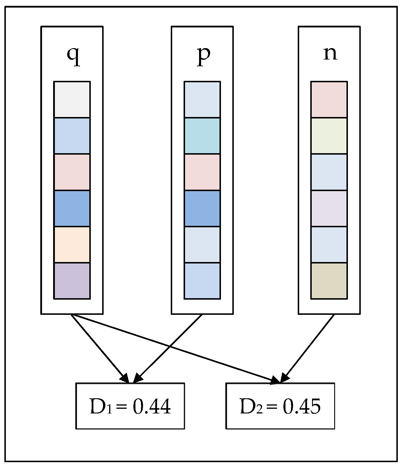
Figure 1.
Each rectangle represents a feature descriptor obtained after the convolution of the neural network. Different colors of small squares represent different feature intensities in the descriptor. The Euclidean distance () between descriptor n and descriptor q is , while the Euclidean distance () between descriptor p and descriptor q is . D1 is approximately equal to D2, but the internal spatial distribution of p and n is obviously different.

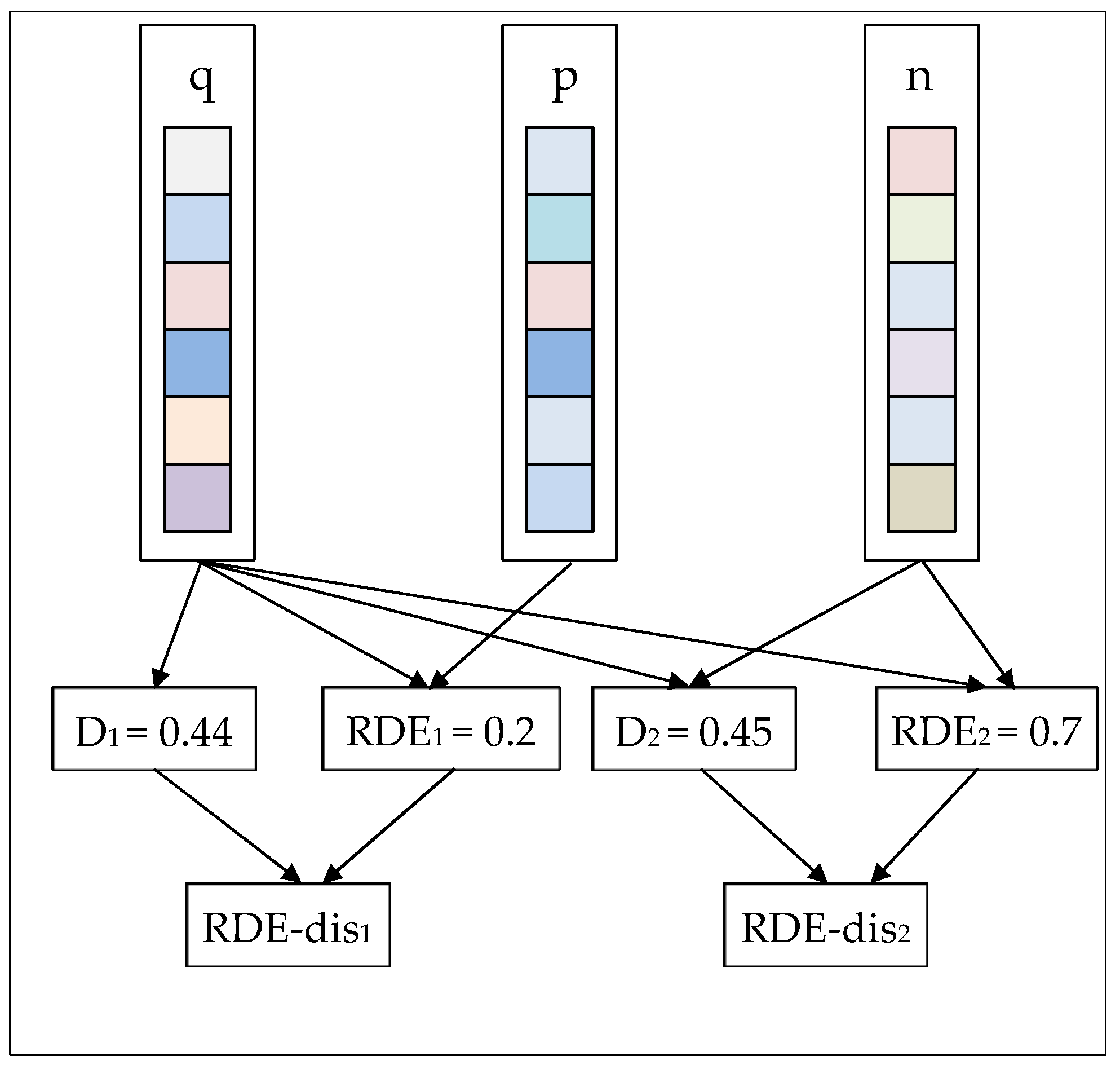
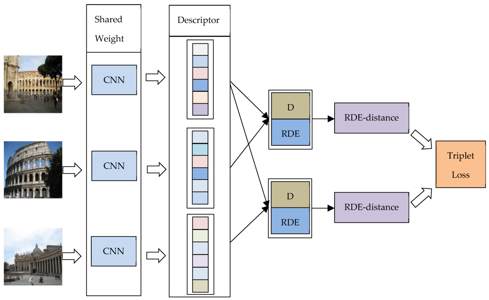
Figure 2.
The core idea of relative distribution entropy (RDE)-loss. D represents the Euclidean distance between two image descriptors. RDE represents the relative distribution entropy between two image descriptors. RDE-distance is a new metric that combines Euclidean distance with relative distributed entropy. We called it the relative distribution entropy weighted distance, which can enhance the discrimination of image descriptors.

Figure 3.
Convolutional neural network (CNN) network architecture.

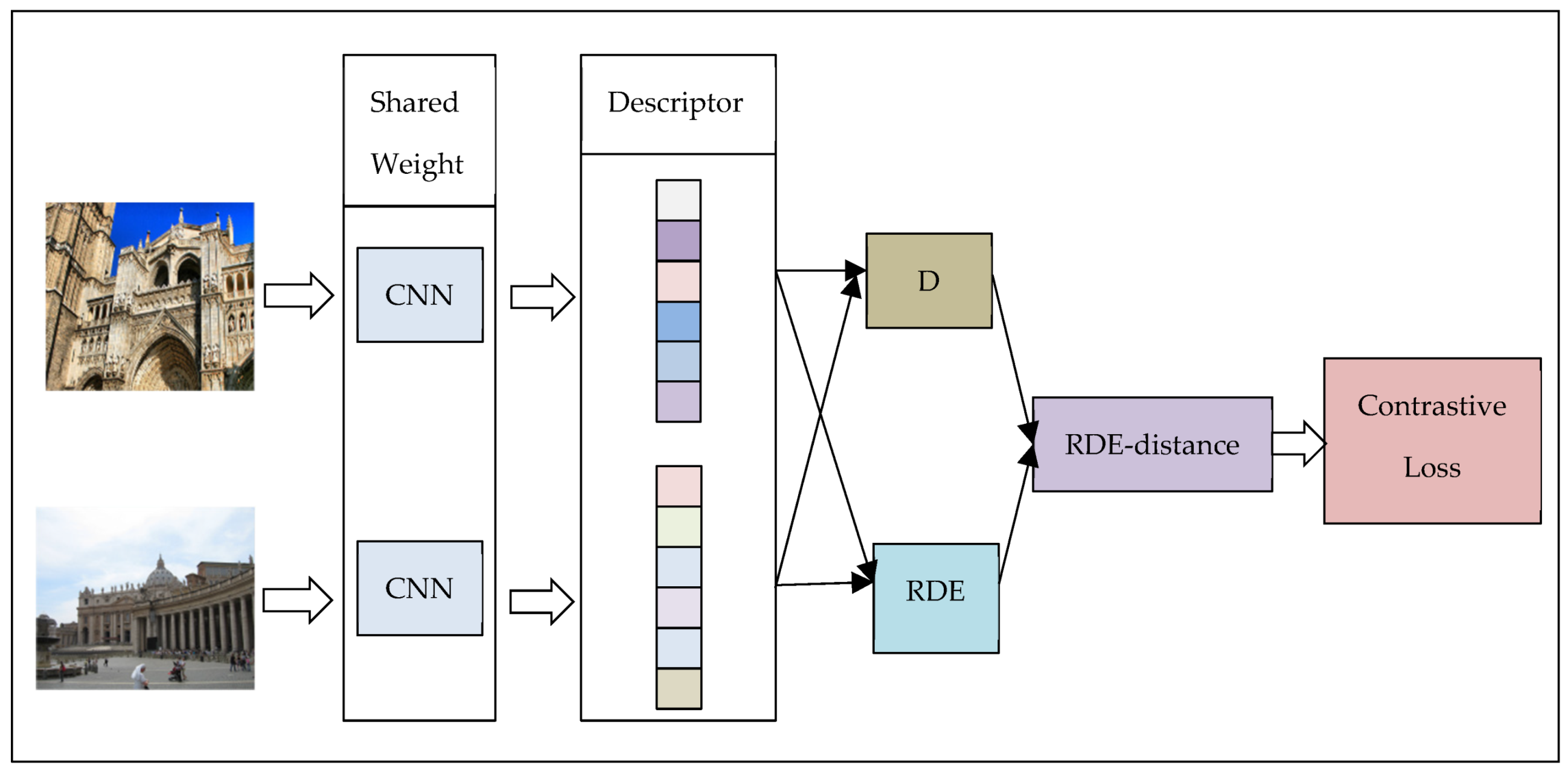
Figure 4.
Training process using relative distribution entropy contrastive loss.

Figure 5.
Training process using relative distribution entropy triplet loss.


Table 1.
Experimental results of hyperparameter comparison in the relative distribution entropy contrastive loss function. The best results would be highlighted in bold.
Table 1.
Experimental results of hyperparameter comparison in the relative distribution entropy contrastive loss function. The best results would be highlighted in bold.
| Network | Oxford5k | Oxford5k(W) | Pairs6k | Pairs6k(W) | ||
|---|---|---|---|---|---|---|
| AlexNet | 0.50 | 10 | 58.10 | 67.60 | 71.64 | 79.60 |
| 0.75 | 20 | 60.87 | 67.19 | 75.33 | 79.43 | |
| 0.85 | 25 | 60.79 | 67.93 | 75.60 | 79.59 | |
| 0.90 | 30 | 61.32 | 68.22 | 75.29 | 80.07 | |
| 1.00 | 50 | 60.27 | 67.72 | 74.88 | 80.10 | |
| VGG | 0.85 | 30 | 84.62 | 87.83 | 82.40 | 88.01 |
| 0.85 | 100 | 76.18 | 83.04 | 81.71 | 87.11 | |
| 0.90 | 30 | 85.09 | 88.00 | 82.69 | 88.12 |
Table 2.
Comparative results of different pooling methods on AlexNet. The best results would be highlighted in bold.
Table 2.
Comparative results of different pooling methods on AlexNet. The best results would be highlighted in bold.
| Net | Oxford5k | Oxford5k(W) | Pairs6k | Pairs6k(W) |
|---|---|---|---|---|
| SPoC [43] | 41.83 | 55.34 | 55.49 | 68.61 |
| MAC [44] | 47.50 | 55.95 | 62.16 | 71.30 |
| GeM [30] | 60.79 | 68.22 | 75.29 | 80.07 |
Table 3.
Performance comparison of relative distribution entropy triplet loss and triplet loss. The best results would be highlighted in bold.
Table 3.
Performance comparison of relative distribution entropy triplet loss and triplet loss. The best results would be highlighted in bold.
| Loss | Network | Oxford5k | Oxford5k(W) | Pairs6k | Pairs6k(W) |
|---|---|---|---|---|---|
| Triplet loss [30] | VGG | 81.48 | 82.80 | 82.79 | 84.78 |
| Ours | 82.39 | 83.07 | 83.61 | 85.45 | |
| Triplet loss [30] | ResNet | 81.49 | 85.33 | 87.70 | 91.11 |
| Ours | 82.88 | 86.54 | 89.33 | 91.97 |
Table 4.
Comparison of our method with the state-of-art image retrieval methods. The best results would be highlighted in bold.
Table 4.
Comparison of our method with the state-of-art image retrieval methods. The best results would be highlighted in bold.
| Net | Method | F-tuned | Oxford5k | Oxford105k | Pairs6k | Pairs106k |
|---|---|---|---|---|---|---|
| VGG | MAC [44] | no | 56.4 | 47.8 | 72.3 | 58.0 |
| SPoC [43] | no | 68.1 | 61.1 | 78.2 | 68.4 | |
| Crow [56] | no | 70.8 | 65.3 | 79.7 | 72.2 | |
| R-MAC [52] | no | 66.9 | 61.6 | 83.0 | 75.7 | |
| BoW-CNN [57] | yes | 73.9 | 59.3 | 82.0 | 64.8 | |
| NetVLAD [58] | yes | 71.6 | - | 79.7 | - | |
| Fisher [59] | yes | 81.5 | 76.6 | 82.4 | - | |
| R-MAC [55] | yes | 83.1 | 78.6 | 87.1 | 79.7 | |
| GeM [30] | yes | 87.9 | 83.3 | 87.7 | 81.3 | |
| ours | yes | 88.0 | 83.5 | 88.1 | 79.9 | |
| Res | R-MAC [52] | no | 69.4 | 63.7 | 85.2 | 77.8 |
| GeM [30] | yes | 87.8 | 84.6 | 92.7 | 86.9 | |
| ours | yes | 88.4 | 84.9 | 92.7 | 86.3 | |
| Re-ranking(R) and Query Expansion(QE) | ||||||
| VGG | Crow + QE [56] | no | 74.9 | 70.6 | 84.8 | 79.4 |
| R-MAC+R+QE [52] | no | 77.3 | 73.2 | 86.5 | 79.8 | |
| BoW-CNN+R+QE [57] | no | 78.8 | 65.1 | 84.8 | 64.1 | |
| R-MAC+QE [55] | yes | 89.1 | 87.3 | 91.2 | 86.8 | |
| GeM+QE [30] | yes | 91.9 | 89.6 | 91.9 | 87.6 | |
| ours | yes | 92.0 | 89.6 | 92.4 | 87.3 | |
| Res | R-MAC+QE [52] | no | 78.9 | 75.5 | 89.7 | 85.3 |
| R-MAC+QE [60] | yes | 90.6 | 89.4 | 96.0 | 93.2 | |
| GeM+QE [30] | yes | 91.0 | 89.5 | 95.5 | 91.9 | |
| ours | yes | 91.7 | 89.7 | 96.0 | 92.1 | |
© 2020 by the authors. Licensee MDPI, Basel, Switzerland. This article is an open access article distributed under the terms and conditions of the Creative Commons Attribution (CC BY) license (http://creativecommons.org/licenses/by/4.0/).
Share and Cite
MDPI and ACS Style
Liu, P.; Shi, L.; Miao, Z.; Jin, B.; Zhou, Q. Relative Distribution Entropy Loss Function in CNN Image Retrieval. Entropy 2020, 22, 321. https://0-doi-org.brum.beds.ac.uk/10.3390/e22030321
AMA Style
Liu P, Shi L, Miao Z, Jin B, Zhou Q. Relative Distribution Entropy Loss Function in CNN Image Retrieval. Entropy. 2020; 22(3):321. https://0-doi-org.brum.beds.ac.uk/10.3390/e22030321
Chicago/Turabian StyleLiu, Pingping, Lida Shi, Zhuang Miao, Baixin Jin, and Qiuzhan Zhou. 2020. "Relative Distribution Entropy Loss Function in CNN Image Retrieval" Entropy 22, no. 3: 321. https://0-doi-org.brum.beds.ac.uk/10.3390/e22030321
Note that from the first issue of 2016, this journal uses article numbers instead of page numbers. See further details here.