On the Rate-Distortion Function of Sampled Cyclostationary Gaussian Processes

Abstract

Man-made communications signals are typically modelled as continuous-time (CT) wide-sense cyclostationary (WSCS) processes. As modern processing is digital, it is applied to discrete-time (DT) processes obtained by sampling the CT processes. When sampling is applied to a CT WSCS process, the statistics of the resulting DT process depends on the relationship between the sampling interval and the period of the statistics of the CT process: When these two parameters have a common integer factor, then the DT process is WSCS. This situation is referred to as synchronous sampling. When this is not the case, which is referred to as asynchronous sampling, the resulting DT process is wide-sense almost cyclostationary (WSACS). The sampled CT processes are commonly encoded using a source code to facilitate storage or transmission over wireless networks, e.g., using compress-and-forward relaying. In this work, we study the fundamental tradeoff between rate and distortion for source codes applied to sampled CT WSCS processes, characterized via the rate-distortion function (RDF). We note that while RDF characterization for the case of synchronous sampling directly follows from classic information-theoretic tools utilizing ergodicity and the law of large numbers, when sampling is asynchronous, the resulting process is not information stable. In such cases, the commonly used information-theoretic tools are inapplicable to RDF analysis, which poses a major challenge. Using the information-spectrum framework, we show that the RDF for asynchronous sampling in the low distortion regime can be expressed as the limit superior of a sequence of RDFs in which each element corresponds to the RDF of a synchronously sampled WSCS process (yet their limit is not guaranteed to exist). The resulting characterization allows us to introduce novel insights on the relationship between sampling synchronization and the RDF. For example, we demonstrate that, differently from stationary processes, small differences in the sampling rate and the sampling time offset can notably affect the RDF of sampled CT WSCS processes.

1. Introduction

Man-made signals are typically generated using a repetitive procedure, which takes place at fixed intervals. The resulting signals are thus commonly modeled as continuous-time (CT) random processes exhibiting periodic statistical properties [1,2,3], which are referred to as wide-sense cyclostationary (WSCS) processes. In digital communications, where the transmitted waveforms commonly obey the WSCS model [3], the received CT signal is first sampled to obtain a discrete-time (DT) received signal. In the event that the sampling interval is commensurate with the period of the statistics of the CT WSCS signal, cyclostationarity is preserved in DT ([3] Section 3.9). In this work, we refer to this situation as synchronous sampling. However, it is practically common to encounter scenarios in which the sampling rate at the receiver and the symbol rate of the received CT WSCS process are incommensurate, which is referred to as asynchronous sampling. The resulting sampled process in such cases is a DT wide-sense almost cyclostationary (WSACS) stochastic process ([3] Section 3.9).

This research aims at investigating lossy source coding for asynchronously sampled CT WSCS processes. In the source coding problem, every sequence of information symbols from the source is mapped into a sequence of code symbols, referred to as codewords, taken from a predefined codebook. In lossy source coding, the source sequence is recovered up to a predefined distortion constraint, within an arbitrary small tolerance of error. The figure-of-merit for lossy source coding is the rate-distortion function (RDF) which characterizes the minimum number of bits per source symbol required to compress the source sequence such that it can be reconstructed at the decoder within the specified maximal distortion [4]. For an independent and identically distributed (IID) random source process, the RDF can be expressed as the minimum mutual information between the source variable and the reconstruction variable, such that with the corresponding conditional distribution of the reconstruction symbol given the source symbol, the distortion constraint is satisfied ([5] Chapter 10). The source coding problem has been further studied in multiple different scenarios, including the reconstruction of a single source at multiple destinations [6] and the reconstruction of multiple correlated stationary Gaussian sources at a single destination [7,8,9].

For sampled stationary source processes, ergodicity theory and the asymptotic equipartition property (AEP) ([5] Chapter 3) were utilized for characterizing the RDF in different scenarios ([10] Chapter 9), ([4] Section I), [11]. However, as in a broad range of applications, including digital communications networks, the CT signals are WSCS processes, the sampling operation results in DT source signals whose statistics depends on the relationship between the sampling rate and the period of the statistics of the source signal. When sampling is synchronous, the resulting DT source signal is WSCS ([3] Section 3.9). The RDF for lossy compression of DT WSCS Gaussian sources with memory was studied in [12]. The work [12] used the fact that any WSCS signal can be transformed into a set of stationary subprocess [2]; thereby facilitating the application of information-theoretic results obtained for multivariate stationary sources to the derivation of the RDF; Nonetheless, in many digital communications scenarios, the sampling rate and the symbol rate of the CT WSCS process are not related in any way, and are possibly incommensurate, resulting in a sampled process which is a DT WSACS stochastic process. Such situations can occur as a result of the a-priori determined values of the sampling interval and the symbol duration of the WSCS source signal, as well as due to sampling clock jitters resulting from hardware impairments. A comprehensive review of trends and applications for almost cyclostationary signals can be found in [13]. Despite of their apparent frequent occurrences, the RDF for lossy compression of WSACS sources has not been characterized, which is the motivation for the current research. A major challenge associated with characterizing fundamental limits for asynchronously sampled WSCS processes stems from the fact that the resulting processes are not information stable, in the sense that their conditional distributions are not ergodic ([14] Page X), [15,16]. As a result, the standard information-theoretic tools cannot be employed, making the characterization of the RDF a very challenging problem.

Our recent study in [17] on channel coding reveals that for the case of additive CT WSCS Gaussian noise, capacity varies significantly with sampling rates, whether the Nyquist criterion is satisfied or not. In particular, it was observed that the capacity can change dramatically with minor variations in the sampling rate, causing it to switch from synchronous sampling to asynchronous sampling. This is in direct contrast to the results obtained for wide-sense stationary noise for which the capacity remains unchanged for any sampling rate above the Nyquist rate [18]. A natural fundamental question that arises from this result is how the RDF of a sampled Gaussian source process varies with the sampling rate. As a motivating example, one may consider compress-and-forward (CF) relaying, in which the relay samples at a rate which can be incommensurate with the symbol rate of the incoming communications signal.

In this work, we employ the information-spectrum framework [14] for characterizing the RDF of asynchronously sampled memoryless Gaussian WSCS processes, as this framework is applicable to the information-theoretic analysis of non information-stable processes ([14] Page VII). We further note that while rate characterizations obtained using information spectrum tools and its associated quantities may be difficult to evaluate ([14] Remark 1.7.3), here we obtain a numerically computable characterization of the RDF. In particular, we focus on the mean squared error (MSE) distortion measure in the low distortion regime, namely, source codes for which the average square of the difference between the source and the reproduction process is not larger than the minimal source variance. The results of this research lead to accurate modelling of signal compression in current and future digital communications systems. The derived RDF, which characterizes the fundamental performance limits in encoding sampled CT WSCS Gaussian processes into a digital representation, allows to evaluate source coding schemes associated with different levels of complexity in terms of their gap from optimality, when applied to this important class of signals.

Furthermore, we utilize our characterization of the RDF to examine how the RDF for a sampled CT WSCS Gaussian source varies with different sampling rates and sampling time offsets. We demonstrate that, differently from stationary sources, when applying a lossy source code to a sampled WSCS process, the achievable rate-distortion tradeoff can be significantly affected by minor variations in the sampling time offset and the sampling rate. Our results thus allow identifying the sampling rate and sampling time offsets which minimize the RDF in systems involving sampled WSCS processes.

The rest of this work is organised as follows: Section 2 provides a scientific background on cyclostationary processes and on rate-distortion analysis of DT WSCS Gaussian sources. Section 3 presents the problem formulation and auxiliary results, and Section 4 details the main result of RDF characterization for sampled WSCS Gaussian process. Numerical examples and discussions are provided in Section 5, and Section 6 concludes the paper.

2. Preliminaries and Background

In the following we review the main tools and framework used in this work: In Section 2.1 we detail the notations, and in Section 2.2 we review the basics of cyclostationary processes and the statistical properties of a DT process resulting from sampling a CT WSCS process. In Section 2.3 we recall some preliminaries of rate-distortion theory as well as the RDF for DT WSCS Gaussian source processes. This background creates a premise for the statement of the main result provided in Section 4 of this paper.

2.1. Notations

In this paper, random vectors are denoted by boldface uppercase letters, e.g., $\mathit{X}$; boldface lowercase letters denote deterministic column vectors, e.g., $\mathit{x}$. Scalar RVs and deterministic values are denoted via standard uppercase and lowercase fonts respectively, e.g., X and x. Scalar random processes are denoted with $X\left(t\right),t\in \mathcal{R}$ for CT and with $X\left[n\right],n\in \mathcal{Z}$ for DT. Uppercase Sans-Serif fonts represent matrices, e.g., $\mathsf{A}$, and the element at the $i^{th}$ row and the $l^{th}$ column of $\mathsf{A}$ is denoted with ${\left(\mathsf{A}\right)}_{i,l}$. We use $|·|$ to denote the absolute value, $\lfloor d\rfloor ,d\in \mathcal{R}$, to denote the floor function and $d^{+},d\in \mathcal{R}$, to denote the $max\{0,d\}$. $\delta [·]$ denotes the Kronecker delta function: $\delta \left[n\right]=1$ for $n=0$ and $\delta \left[n\right]=0$ otherwise, and $\mathbb{E}\{·\}$ denotes the stochastic expectation. The sets of positive integers, integers, rational numbers, real numbers, positive numbers, and complex numbers are denoted by $\mathcal{N},\mathcal{Z}$, $\mathcal{Q}$, $\mathcal{R}$, ${\mathcal{R}}^{++}$, and $\mathcal{C}$, respectively. The cumulative distribution function (CDF) is denoted by $F_X\left(x\right)\triangleq Pr(X\le x)$ and the probability density function (PDF) of a CT random variable (RV) is denoted by $p_X\left(x\right)$. We represent a real Gaussian distribution with mean $\mu$ and variance ${\sigma }^2$ by the notation $\mathcal{N}(\mu ,{\sigma }^2)$. All logarithms are taken to base-2, and $j=\sqrt{-1}$. Lastly, for any sequence $y\left[i\right]$, $i\in \mathcal{N}$, and positive integer $k\in \mathcal{N}$, ${\mathit{y}}^{\left(k\right)}$ denotes the column vector ${\left(y\left[1\right],\dots ,y\left[k\right]\right)}^T$.

2.2. Wide-Sense Cyclostationary Random Processes

Here, we review some preliminaries from the theory of cyclostationarity. We begin by recalling the definition of wide-sense cyclostationary processes for CT and for DT:

Definition 1

(CT wide-sense cyclostationary processes ([3] Section 3.2.1)). A scalar stochastic process ${\{S\left(t\right)\}}_{t\in \mathcal{R}}$ is called WSCS if both its first-order and its second-order moments are periodic with respect to $t\in \mathcal{R}$ with some period $T_p\in \mathcal{R}$.

Definition 2

(DT wide-sense cyclostationary processes ([2] Section 17.2)). A scalar stochastic process ${\{S\left[n\right]\}}_{n\in \mathcal{Z}}$ is called WSCS if both its first-order and its second-order moments are periodic with respect to $n\in \mathcal{Z}$ with some period $N_p\in \mathcal{Z}$.

WSCS signal are thus random processes whose first and second-order moments are periodic functions with the same period. To define WSACS signals, we first recall the definition of almost-periodic functions:

Definition 3

(Almost-periodic functions ([19] Definition 2.1)). A DT function $x\left[n\right]$, $n\in \mathcal{Z}$, is called an almost-periodic function if for every $ϵ>0$ there exists a number $l\left(ϵ\right)\in \mathcal{N}$ with the property that for any $n\in \mathcal{Z}$ and any $\alpha \in \mathcal{Z}$, $\exists \Delta \in \left[\alpha ,\alpha +l\left(ϵ\right)\right]$, such that

$$\left|x\right[\Delta ]-x[n\left]\right|<ϵ.$$

Definition 4

(DT wide-sense almost-cyclostationary processes ([2] Section 17.2)). A scalar stochastic process ${\left\{S\left[n\right])\right\}}_{n\in \mathcal{Z}}$ is called WSACS if its first and its second order moments are almost-periodic functions with respect to $n\in \mathcal{Z}$.

Remark 1.

Note that when the mean and the autocorrelation function are each periodic with periods which are incommensurate, the resulting processes is WSACS. We note that in many practical cases the mean is zero, see e.g., ([2] Section 17.2), hence the classification of the process will be determined by the periodicity of the autocorrelation function.

The DT WSCS model is commonly used in the communications literature, as it facilitates the the analysis of many problems of interest, such as fundamental rate limits analysis [20,21,22], channel identification [23], synchronization [24], and noise mitigation [25]. However, in many scenarios, the considered signals are WSACS rather than WSCS. To see how the WSACS model is obtained in the context of sampled signals, we briefly recall the discussion in [17] on sampled WSCS processes (please refer to ([17] Section II.B) for more details): Consider a CT WSCS random process $S\left(t\right)$, which is sampled uniformly with a sampling interval of $T_{\mathrm{s}}$ and sampling time offset $\varphi$, resulting in a DT random process $S\left[i\right]=S(i·T_{\mathrm{s}}+\varphi )$. It is well known that contrary to stationary processes, which have a time-invariant statistical characteristics, the values of $T_{\mathrm{s}}$ and $\varphi$ have a significant effect on the statistics of sampled WSCS processes ([17] Section II.B). To demonstrate this point, consider a CT WSCS process with variance ${\sigma }_s^2\left(t\right)=\frac{1}{2}·sin\left(2\pi t/T_{\mathrm{sym}}\right)+2$ for some $T_{\mathrm{sym}}>0$. The sampled process for $\varphi =0$ (no sampling time offset) and $T_{\mathrm{s}}=\frac{T_{\mathrm{sym}}}{3}$ has a variance function whose period is $N_p=3$: ${\sigma }_s^2\left(i{T}_{\mathrm{s}}\right)=\{2,2.433,1.567,2,2.433,1.567,\dots \}$, for $i=0,1,2,3,4,5,\dots$; while the DT process obtained with the same sampling interval and with a sampling time offset of $\varphi =\frac{T_{\mathrm{s}}}{2\pi }$ has a periodic variance with $N_p=3$ with values ${\sigma }_s^2(i{T}_{\mathrm{s}}+\varphi )=\{2.155,2.335,1.510,2.155,2.335,1.510,\dots \}$, for $i=0,1,2,3,4,5,\dots$, which are different from the values of the DT variance for $\varphi =0$. It follows that both variances are periodic in discrete-time with the same period $N_p=3$, although with different values within the period, which is a result of the sampling time offset, yet, both DT processes correspond to two instances of synchronous sampling. Lastly, consider the sampled variance obtained by sampling without a time offset (i.e., $\varphi =0$) at a sampling interval of $T_{\mathrm{s}}=(1+\frac{1}{2\pi })\frac{T_{\mathrm{sym}}}{3}$. For this case, $T_{\mathrm{s}}$ is not an integer divisor of $T_{\mathrm{sym}}$ or of any of its integer multiples (i.e., $\frac{T_{\mathrm{sym}}}{T_{\mathrm{s}}}=2+\frac{2\pi -2}{2\pi +1}\equiv 2+ϵ$; where $ϵ\notin \mathcal{Q}$ and $ϵ\in [0,1)$) resulting in the variance values ${\sigma }_s^2\left(i{T}_{\mathrm{s}}\right)=\{2,2.335,1.5027,2.405,1.896,1.75,\dots \}$, for $i=0,1,2,3,4,5\dots$. For this scenario, the DT variance is not periodic but is almost-periodic, corresponding to asynchronous sampling and the resulting DT process is not WSCS but WSACS ([3] Section 3.2). The example above demonstrates that the statistical properties of sampled WSCS processes depend on the sampling rate and the sampling time offset, implying that the RDF of such processes should also depend on these quantities, as we demonstrate in the sequel.

2.3. The Rate-Distortion Function for DT WSCS Processes

In this subsection we review the source coding problem and the existing results on the RDF of WSCS processes. We begin by recalling the definition of a source coding scheme, see, e.g., ([26] Chapter 30), ([5] Chapter 10):

Definition 5

(Source coding scheme). A source coding scheme with blocklength l consists of (see Figure 1):

1. 

An encoder$f_S$which maps a block of l source samples${\{S\left[i\right]\}}_{i=1}^l$into an index from a set of$M=2^{lR}$indexes,$f_S:{\{S\left[i\right]\}}_{i=1}^l\mapsto \{1,2,\dots ,M\}$.

2. 

A decoder$g_S$which maps the received index into a reconstructed sequence of length l,${\left\{\widehat{S}\left[i\right]\right\}}_{i=1}^l$,$g_S:\{1,2,\dots ,M\}\mapsto {\left\{\widehat{S}\left[i\right]\right\}}_{i=1}^l$

The encoder-decoder pair is referred to as an$(R,l)$source code, where R is the rate of the code in bits per source symbol, defined as:

$$R=\frac{1}{l}{log}_{2}M$$

(1)

The RDF characterizes the minimal average number of bits per source symbol, denoted $R\left(D\right)$, that can be used to encode a source process such that it can be reconstructed from its encoded representation with a recovery distortion not larger than $D>0$ ([5] Section 10.2). In the current work, we use the MSE distortion measure, which measures the distortion due to decoding a source symbol S into $\widehat{S}$ via $d(S,\widehat{S})={(S-\widehat{S})}^2$. The distortion for a sequence of source samples ${\mathit{S}}^{(l)}$ decoded into a reproduction sequence ${\widehat{\mathit{S}}}^{(l)}$ is given by $d\left({\mathit{S}}^{(l)},{\widehat{\mathit{S}}}^{(l)}\right)=\frac{1}{l}{\displaystyle \sum _{i=1}^l}{\left(S\left[i\right]-\widehat{S}\left[i\right]\right)}^2$ and the average distortion in decoding a random source sequence ${\mathit{S}}^{(l)}$ into a random reproduction sequence ${\widehat{\mathit{S}}}^{(l)}$ is defined as:

$$\overline{d}\left({\mathit{S}}^{(l)},{\widehat{\mathit{S}}}^{(l)}\right)\triangleq \mathbb{E}\left\{d\left({\mathit{S}}^{(l)},{\widehat{\mathit{S}}}^{(l)}\right)\right\}=\frac{1}{l}\sum _{i=1}^l\mathbb{E}\left\{{\left(S\left[i\right]-\widehat{S}\left[i\right]\right)}^2\right\},$$

(2)

where the expectation in Equation (2) is taken with respect to the joint probability distributions on the source $S\left[i\right]$ and its reproduction $\widehat{S}\left[i\right]$. Using Definition 5 we can now define the achievable rate-distortion pair for a source $S\left[i\right]$, as stated in the following definition ([10] Pg. 471):

Definition 6

(Achievable rate-distortion pair). A rate-distortion pair $(R,D)$ is achievable for a process ${\{S\left[i\right]\}}_{i\in \mathcal{N}}$ if for any $\eta >0$ and for all sufficiently large l it is possible to construct an $\left(R_s,l\right)$ source code such that

$$R_s\le R+\eta .$$

(3)

and

$$\overline{d}\left({\mathit{S}}^{(l)},{\widehat{\mathit{S}}}^{(l)}\right)\le D+\eta .$$

(4)

Definition 7.

The rate-distortion function$R(D)$is defined as the infimum of all achievable rates R for a given maximum allowed distortion D.

Definition 6 defines a rate-distortion pair to be achievable if the rate and the distortion constraints are satisfied using source codes with any sufficiently large blocklength. In the following lemma, which will be used to characterize the RDF of DT WSCS signals, we state that it is sufficient to consider only source codes whose blocklength is an integer multiple of some fixed positive integer:

Lemma 1.

Consider the process${\{S\left[i\right]\}}_{i\in \mathcal{N}}$with a finite and bounded variance. For a given maximum allowed distortion D, the optimal reproduction process${\{\widehat{S}\left[i\right]\}}_{i\in \mathcal{N}}$is also the optimal reproduction process when restricted to using source codes whose blocklengths are integer multiples of some fixed positive integer r.

Proof. 

The proof of the lemma is detailed in Appendix A. □

This lemma facilitates switching between multivariate and scalar representations of the source and the reproduction processes.

The RDF obviously depends on the distribution of the source ${\{S\left[i\right]\}}_{i\in \mathcal{N}}$. Thus, statistically different sources have different RDFs. However, when a source is scaled by some positive constant, the RDF of the scaled process with the MSE distortion can be inferred from that of the original source process, as stated in the following theorem:

Theorem 1.

Let${\{S\left[i\right]\}}_{i\in \mathcal{N}}$be a source process for which the rate-distortion pair$(R,D)$is achievable under the MSE distortion. Then, for every$\alpha \in {\mathcal{R}}^{++}$, it holds that the rate-distortion pair$(R,{\alpha }^2·D)$is achievable for the scaled source${\{\alpha ·S\left[i\right]\}}_{i\in \mathcal{N}}$.

Proof. 

The proof of the theorem is detailed in Appendix B. □

Lastly, in the proof of our main result, we make use of the RDF for DT WSCS sources derived in ([12] Theorem 1), repeated below for ease of reference. Prior to the statement of the theorem, we recall that for blocklenghts which are integer multiples of $N_p$, a WSCS process $S\left[i\right]$ with period $N_p>0$ can be represented as an equivalent $N_p$-dimensional process ${\mathit{S}}^{(N_p)}\left[i\right]$ via the decimated component decomposition (DCD) ([2] Section 17.2). The power spectral density (PSD) of the process ${\mathit{S}}^{(N_p)}$ is defined as ([12] Section II):

$${\left({\rho }_{\mathit{S}}\left(e^{j2\pi f}\right)\right)}_{u,v}=\sum _{\Delta \in \mathcal{Z}}{\left({\mathsf{R}}_{\mathit{S}}[\Delta ]\right)}_{u,v}{e}^{-j2\pi f\Delta }-\frac{1}{2}\le f\le \frac{1}{2},u,v\in \{1,2,\dots N_p\}$$

(5)

where ${\mathsf{R}}_{\mathit{S}}[\Delta ]\triangleq \mathbb{E}\left\{{\mathit{S}}^{(N_p)}\left[i\right]·{\mathit{S}}^{(N_p)}[i+\Delta ]\right\}$ ([2] Section 17.2). We now proceed to the statement of ([12] Theorem 1):

Theorem 2.

([12] Theorem 1) Consider a zero-mean real DT WSCS Gaussian source$S\left[i\right],i\in \mathcal{N}$with memory, and let$N_p\in \mathcal{N}$denote the period of its statistics. The RDF is expressed as:

$$R(D)=\frac{1}{2N_p}\sum _{m=1}^{N_p}{\int }_{f=-0.5}^{0.5}{\left(log\left(\frac{{\lambda }_m\left(e^{j2\pi f}\right)}{\theta }\right)\right)}^{+}\mathrm{d}f,$$

(6a)

where${\lambda }_m\left(e^{j2\pi f}\right)$,$m=1,2,\dots ,N_p$denote the eigenvalues of the PSD matrix of the process${\mathit{S}}^{(N_p)}\left[i\right]$, which is obtained from$S\left[i\right]$by applying the$N_p$-dimensional DCD, and θ is selected such that

$$D=\frac{1}{N_p}\sum _{m=1}^{N_p}{\int }_{f=-0.5}^{0.5}min\left\{{\lambda }_m\left(e^{j2\pi f}\right),\theta \right\}\mathrm{d}f.$$

(6b)

We note that ${\mathit{S}}^{(N_p)}\left[i\right]$ corresponds to a vector of stationary processes whose elements are not identically distributed; hence the variance function is different for each scalar stationary process. Using ([12] Theorem 1), we can directly obtain the RDF for the special case of a DT memoryless WSCS Gaussian process. This is stated in the following corollary:

Corollary 1.

Let${\{S\left[i\right]\}}_{i\in \mathcal{N}}$be a zero-mean DT memoryless real WSCS Gaussian source with period$N_p\in \mathcal{N}$, and set${\sigma }_m^2=\mathbb{E}\{S^2\left[m\right]\}$for$m=1,2,\dots ,N_P$. The RDF for compression of$S\left[i\right]$is expressed as:

$$\begin{array}{c}\hfill R(D)=\left\{\begin{array}{cc}\frac{1}{2N_p}{\displaystyle \sum _{m=1}^{N_p}}log\left(\frac{{\sigma }_m^2}{D_m}\right)\hfill & D\le \frac{1}{N_p}{\displaystyle \sum _{m=1}^{N_p}}{\sigma }_m^2\hfill \\ 0\hfill & D>\frac{1}{N_p}{\displaystyle \sum _{m=1}^{N_p}}{\sigma }_m^2,\hfill \end{array}\right.\end{array}$$

(7a)

where$D_m\triangleq min\left\{{\sigma }_m^2,\theta \right\}$, and θ is defined such that

$$D=\frac{1}{N_p}\sum _{m=1}^{N_p}{D}_m.$$

(7b)

Proof. 

Applying Equations (6a) and (6b) to our specific case of a memoryless WSCS source, we obtain Equations (7a) and (7b) as follows: First, note that the corresponding DCD components for a zero-mean memoryless WSCS process are also zero-mean and memoryless; hence the PSD matrix for the multivariate process ${\mathit{S}}^{(N_p)}\left[i\right]$ is a diagonal matrix, whose eigenvalues are the constant diagonal elements such that the mth diagonal element is equal to the variance ${\sigma }_m^2$: ${\lambda }_m\left(e^{j2\pi f}\right)={\sigma }_m^2$. Now, writing Equation (6a) for this case we obtain:

$$\begin{array}{cc}\hfill R(D)& =\frac{1}{2N_p}\sum _{m=1}^{N_p}{\int }_{f=-0.5}^{0.5}{\left(log\left(\frac{{\lambda }_m\left(e^{j2\pi f}\right)}{\theta }\right)\right)}^{+}\mathrm{d}f\hfill \\ \hfill & =\frac{1}{2N_p}\sum _{m=1}^{N_p}{\left(log\left(\frac{{\sigma }_m^2}{\theta }\right)\right)}^{+}.\hfill \end{array}$$

(8)

Since ${\left(log\left(\frac{{\sigma }_m^2}{\theta }\right)\right)}^{+}=max\left\{0,log\left(\frac{{\sigma }_m^2}{\theta }\right)\right\}\equiv log\left(\frac{{\sigma }_m^2}{D_m}\right)$ it follows that (8) coincides with (7a). Next, expressing Equation (6b) for the memoryless source process, we obtain:

$$D=\frac{1}{N_p}\sum _{m=1}^{N_p}{\int }_{f=-0.5}^{0.5}min\left\{{\lambda }_m\left(e^{j2\pi f}\right),\theta \right\}\mathrm{d}f=\frac{1}{N_p}\sum _{m=1}^{N_p}min\left\{{\sigma }_m^2,\theta \right\},$$

(9)

proving Equation (7b). □

Now, from Lemma 1, we conclude that the RDF for compression of source sequences whose blocklength is an integer multiple of $N_p$ is the same as the RDF for compressing source sequences whose blocklength is arbitrary. We recall that from ([5] Chapter 10.3.3) it follows that for the zero-mean memoryless Gaussian DCD vector source process ${\mathit{S}}^{(N_p)}\left[i\right]$ the optimal reproduction process which achieves the RDF is an $N_p\times 1$ memoryless process whose covariance matrix is diagonal with non-identically distributed elements. From [2], we can apply the inverse DCD to obtain a WSCS process. Hence, from Lemma 1 we can conclude that the optimal reproduction process for the DT WSCS Gaussian source is a DT WSCS Gaussian process.

3. Problem Formulation and Auxiliary Results

Our objective is to characterize the RDF for compression of asynchronously sampled CT WSCS Gaussian sources when the sampling interval is larger than the memory of the source. In particular, we focus on the minimal rate required to achieve a high fidelity reproduction, representing the RDF curve for distortion values not larger than the variance of the source. Such characterization of the RDF for asynchronous sampling is essential for comprehending the relationship between the minimal required number of bits and the sampling rate at a given distortion. Our analysis constitutes an important step towards constructing joint source-channel coding schemes for scenarios in which the symbol rate of the transmitter is not necessarily synchronized with the sampling rate of the source to be transmitted. Such scenarios arise, for example, when recording a communications signal for storage or processing, or in compress-and-forward relaying (([26] Chapter 16.7), [27]) in which the relay compresses the sampled received signal, which is then forwarded to the assisted receiver. As the relay operates with its own sampling clock, which need not necessarily be synchronized with the symbol rate of the assisted transmitter, sampling at the relay may result in a DT WSACS source signal. In the following we first characterize the sampled source model in Section 3.1. Then, as a preliminary step towards our characterization the RDF for asynchronously sampled CT WSCS Gaussian processes stated in Section 4, we recall in Section 3.2 the definitions of some information-spectrum quantities used in this study. Finally, in Section 3.3, we recall an auxiliary result relating the information-spectrum quantities of a collection of sequences of RVs to the information-spectrum quantities of its limit sequence of RVs. This result will be applied in the derivation of the RDF with asynchronous sampling.

3.1. Source Model

Consider a real CT, zero-mean WSCS Gaussian random process $S_c(t)$ with period $T_{\mathrm{ps}}$. Let the variance function of $S_c(t)$ be defined as ${\sigma }_{S_{\mathrm{c}}}^2(t)\triangleq \mathbb{E}\left\{S_{\mathrm{c}}^2(t)\right\}$, and assume it is both upper bounded and lower bounded away from zero, and that it is continuous in $t\in \mathcal{R}$. Let ${\tau }_m>0$ denote the maximal correlation length of $S_c(t)$, i.e., $r_{S_c}(t,\tau )\triangleq \mathbb{E}\left\{S_c(t)S_c(t-\tau )\right\}=0,\forall \left|\tau \right|>{\tau }_m$. By the cyclostationarity of $S_{\mathrm{c}}(t)$, we have that ${\sigma }_{S_c}^2(t)={\sigma }_{S_c}^2(t+T_{\mathrm{ps}}),\forall t\in \mathcal{R}$. Let $S_c(t)$ be sampled uniformly with the sampling interval $T_{\mathrm{s}}>0$ such that $T_{\mathrm{ps}}=(p+ϵ)·T_{\mathrm{s}}$ for $p\in \mathcal{N}$ and $ϵ\in [0,1)$ yielding $S_{ϵ}\left[i\right]\triangleq S_{\mathrm{c}}(i·T_{\mathrm{s}})$, where $i\in \mathcal{Z}$. The variance of $S_{ϵ}\left[i\right]$ is given by ${\sigma }_{S_{ϵ}}^2\left[i\right]\triangleq r_{S_{ϵ}}[i,0]={\sigma }_{S_{\mathrm{c}}}^2\left(\frac{i·T_{\mathrm{ps}}}{p+ϵ}\right)$.

In this work, as in [17], we assume that the duration of temporal correlation of the CT signal is shorter than the sampling interval $T_{\mathrm{s}}$, namely, ${\tau }_m<T_{\mathrm{s}}$. Consequently, the DT Gaussian process $S_{ϵ}\left[i\right]$ is a memoryless zero-mean Gaussian process and its autocorrelation function is given by:

$$\begin{array}{cc}\hfill r_{S_{ϵ}}[i,\Delta ]& =\mathbb{E}\left\{S_{ϵ}\left[i\right]S_{ϵ}[i+\Delta ]\right\}\hfill \\ & =\mathbb{E}\left\{S_{\mathrm{c}}\left(\frac{i·T_{\mathrm{ps}}}{p+ϵ}\right)·S_{\mathrm{c}}\left(\frac{(i+\Delta )·T_{\mathrm{ps}}}{p+ϵ}\right)\right\}={\sigma }_{S_{\mathrm{c}}}^2\left(\frac{i·T_{\mathrm{ps}}}{p+ϵ}\right)·\delta [\Delta ]={\sigma }_{S_{ϵ}}^2\left[i\right]·\delta [\Delta ].\hfill \end{array}$$

(10)

While we do not explicitly account for sampling time offsets in our definition of the sampled process $S_{ϵ}\left[i\right]$, it can be incorporated by replacing ${\sigma }_{S_{\mathrm{c}}}^2(t)$ with a time-shifted version, i.e., ${\sigma }_{S_{\mathrm{c}}}^2(t-\varphi )$, see also ([17] Section II.C).

It can be noted from (10) that if $ϵ$ is a rational number, i.e., $\exists u,v\in \mathcal{N}$, u and v are relatively prime, such that $ϵ=\frac{u}{v}$, then ${\left\{S_{ϵ}\left[i\right]\right\}}_{i\in \mathcal{Z}}$ is a DT memoryless WSCS process with the period $p_{u,v}=p·v+u\in \mathcal{N}$ ([17] Section II.C). For this class of processes, the RDF can be obtained from ([12] Theorem 1) as stated in Corollary 1. On the other hand, if $ϵ$ is an irrational number, then sampling becomes asynchronous and leads to a WSACS process whose RDF has not been characterized to date.

3.2. Definitions of Relevant Information-Spectrum Quantities

Conventional information theoretic tools for characterizing RDFs are based on an underlying ergodicity of the source. Consequently, these techniques cannot be applied to characterize the RDF of asynchronously sampled WSCS processes. To tackle this challenge, we use the information-spectrum framework, as this framework [14] can be utilized to obtain general formulas for rate limits for any arbitrary class of processes. The resulting expressions are not restricted to specific statistical models of the considered processes, and in particular, do not require information stability or stationarity. In the following, we recall the definitions of several information-spectrum quantities used in this study, see also ([14] Definitions 1.3.1 and 1.3.2):

Definition 8.

The limit-inferior in probability of a sequence of real RVs${\{Z_k\}}_{k\in \mathcal{N}}$is defined as

$$\mathrm{p}-\underset{k\to \infty }{liminf}{Z}_k\triangleq sup\left\{\alpha \in \mathcal{R}|\underset{k\to \infty }{lim}Pr\left(Z_k<\alpha \right)=0\right\}\triangleq {\alpha }_0.$$

(11)

Hence, ${\alpha }_0$ is the largest real number satisfying that $\forall \tilde{\alpha }<{\alpha }_0$ and $\forall \mu >0$ there exists $k_0(\mu ,\tilde{\alpha })\in \mathcal{N}$ such that $Pr(Z_k<\tilde{\alpha })<\mu$, $\forall k>k_0(\mu ,\tilde{\alpha })$.

Definition 9.

The limit-superior in probability of a sequence of real RVs${\{Z_k\}}_{k\in \mathcal{N}}$is defined as

$$\mathrm{p}-\underset{k\to \infty }{limsup}{Z}_k\triangleq inf\left\{\beta \in \mathcal{R}|\underset{k\to \infty }{lim}Pr\left(Z_k>\beta \right)=0\right\}\triangleq {\beta }_0.$$

(12)

Hence, ${\beta }_0$ is the smallest real number satisfying that $\forall \tilde{\beta }>{\beta }_0$ and $\forall \mu >0$, there exists $k_0(\mu ,\tilde{\beta })\in \mathcal{N}$, such that $Pr(Z_k>\tilde{\beta })<\mu$, $\forall k>k_0(\mu ,\tilde{\beta })$.

The notion of uniform integrability of a sequence of RVs is a basic property in probability ([28] Chapter 12), which is not directly related to information spectrum methods. However, since it plays an important role in the information spectrum characterization of RDFs, we include its statement in the following definition:

Definition 10

(Uniform integrability ([28] Definition 12.1), ([14] Equation (5.3.2))). The sequence of real-valued random variables ${\{Z_k\}}_{k=1}^{\infty }$, is said to satisfy uniform integrability if

$$\underset{u\to \infty }{lim}\underset{k\ge 1}{sup}\underset{z:|z|\ge u}{\int }{p}_{Z_k}\left(z\right)|z|\mathrm{d}z=0$$

(13)

The aforementioned quantities facilitate characterizing the RDF of arbitrary sources. Consider a general source process ${\{S\left[i\right]\}}_{i=1}^{\infty }$ (stationary or non-stationary) taking values from the source alphabet $S\left[i\right]\in \mathcal{S}$ and a reproduction process ${\{\widehat{S}\left[i\right]\}}_{i=1}^{\infty }$ with values from the reproduction alphabet $\widehat{S}\left[i\right]\in \widehat{\mathcal{S}}$. It follows from ([14] Section 5.5) that for a distortion measure which satisfies the uniform integrability criterion, i.e., that there exists a deterministic sequence ${\{r\left[i\right]\}}_{i=1}^{\infty }$ such that the sequence of RVs ${\{d\left({\mathit{S}}^{(k)},{\mathit{r}}^{(k)}\right)\}}_{k=1}^{\infty }$ satisfies Definition 10 ([14] Page 336), then the RDF is expressed as ([14] Equation (5.4.2)):

$$R(D)=\underset{F_{S,\widehat{S}}:{\overline{d}}_S({\mathit{S}}^{(k)},{\widehat{\mathit{S}}}^{(k)})\le D}{inf}\overline{I}\left({\mathit{S}}^{(k)};{\widehat{\mathit{S}}}^{(k)}\right),$$

(14)

where ${\overline{d}}_S({\mathit{S}}^{(k)},{\widehat{\mathit{S}}}^{(k)})=\underset{k\to \infty }{limsup}\mathbb{E}\left\{d\left({\mathit{S}}^{(k)},{\widehat{\mathit{S}}}^{(k)}\right)\right\}$, $F_{S,\widehat{S}}$ denotes the joint CDF of ${\{S\left[i\right]\}}_{i=1}^{\infty }$ and ${\{\widehat{S}\left[i\right]\}}_{i=1}^{\infty }$, and $\overline{I}\left({\mathit{S}}^{(k)}:{\widehat{\mathit{S}}}^{(k)}\right)$ represents the limit superior in probability of the mutual information rate of ${\mathit{S}}^{(k)}$ and ${\widehat{\mathit{S}}}^{(k)}$, given by:

$$\overline{I}\left({\mathit{S}}^{(k)};{\widehat{\mathit{S}}}^{(k)}\right)\triangleq \mathrm{p}-\underset{k\to \infty }{limsup}\frac{1}{k}log\frac{p_{{\mathit{S}}^{(k)}|{\widehat{\mathit{S}}}^{(k)}}\left({\mathit{S}}^{(k)}|{\widehat{\mathit{S}}}^{(k)}\right)}{p_{{\mathit{S}}^{(k)}}\left({\mathit{S}}^{(k)}\right)}$$

(15)

In order to use the RDF characterization in (14), the distortion measure must satisfy the uniform integrability criterion. For the considered class of sources detailed in Section 3.1, the MSE distortion satisfies this criterion, as stated in the following lemma:

Lemma 2.

For any real memoryless zero-mean Gaussian source${\{S\left[i\right]\}}_{i=1}^{\infty }$with bounded variance, i.e.,$\exists {\sigma }_{max}^2<\infty$such that$\mathbb{E}\{S^2\left[i\right]\}\le {\sigma }_{max}^2$for all$i\in \mathcal{N}$, the MSE distortion satisfies the uniform integrability criterion.

Proof. 

Set the deterministic sequence ${\{r\left[i\right]\}}_{i=1}^{\infty }$ to be the all-zero sequence. Under this setting and the MSE distortion, it holds that $d\left({\mathit{S}}^{(k)},{\mathit{r}}^{(k)}\right)=\frac{1}{k}{\sum }_{i=1}^k{S}^2\left[i\right]$. To prove the lemma, we show that the sequence of RVs ${\left\{d\left({\mathit{S}}^{(k)},{\mathit{r}}^{(k)}\right)\right\}}_{k=1}^{\infty }$ has a bounded ${\ell }_2$ norm, which implies that it is uniformly integrable by ([28] Corollary 12.8). The ${\ell }_2$ norm of $d\left({\mathit{S}}^{(k)},{\mathit{r}}^{(k)}\right)$ satisfies

$$\begin{array}{cc}\hfill \mathbb{E}\left\{d{\left({\mathit{S}}^{(k)},{\mathit{r}}^{(k)}\right)}^2\right\}& =\frac{1}{k^2}\mathbb{E}\left\{\sum _{i=1}^k{S}^2\left[i\right]\sum _{j=1}^k{S}^2\left[j\right]\right\}\hfill \\ \hfill & =\frac{1}{k^2}\sum _{i=1}^k\sum _{j=1}^k\mathbb{E}\left\{S^2\left[i\right]S^2\left[j\right]\right\}\stackrel{(a)}{\le }\frac{1}{k^2}\sum _{i=1}^k\sum _{j=1}^{k}3{\sigma }_{max}^4=3{\sigma }_{max}^4,\hfill \end{array}$$

(16)

where $(a)$ follows since $\mathbb{E}\{S^2\left[i\right]S^2\left[j\right]\}=\mathbb{E}\{S^2\left[i\right]\}\mathbb{E}\{S^2\left[j\right]\}={\sigma }_{max}^4$ for $i\ne j$ while $\mathbb{E}\{S^4\left[i\right]\}=3{\sigma }_{max}^4$ ([29] Chapter 5.4). Equation (16) proves that $d\left({\mathit{S}}^{(k)},{\mathit{r}}^{(k)}\right)$ is ${\ell }_2$-bounded by $3{\sigma }_{max}^4<\infty$ for all $k\in \mathcal{N}$, which in turn implies that the MSE distortion is uniformly integrable for the source ${\{S\left[i\right]\}}_{i=1}^{\infty }$. □

Since, as detailed in Section 3.1, we focus in the following on memoryless zero-mean Gaussian sources, Lemma 2 implies that the RDF of the source can be characterized using (14). However, (14) is in general difficult to evaluate, and thus does not lead to a meaningful understanding of how the RDF of sampled WSCS sources behaves, motivating our analysis in Section 4.

3.3. Information Spectrum Limits

The following theorem originally stated in ([17] Theorem 1) presents a fundamental result which is directly useful for the derivation of the RDF:

Theorem 3.

([17] Theorem 1) Let${\left\{{\tilde{Z}}_{k,n}\right\}}_{n,k\in \mathcal{N}}$be a set of sequences of real scalar RVs satisfying two assumptions:

AS1 

For every fixed$n\in \mathcal{N}$, every convergent subsequence of${\left\{{\tilde{Z}}_{k,n}\right\}}_{k\in \mathcal{N}}$converges in distribution, as$k\to \infty$, to a finite deterministic scalar. Each subsequence may converge to a different scalar.

AS2 

For every fixed$k\in \mathcal{N}$, the sequence${\left\{{\tilde{Z}}_{k,n}\right\}}_{n\in \mathcal{N}}$converges uniformly in distribution, as$n\to \infty$, to a scalar real-valued RV$Z_k$. Specifically, letting${\tilde{F}}_{k,n}(\alpha )$and$F_k(\alpha )$,$\alpha \in \mathcal{R}$, denote the CDFs of${\tilde{Z}}_{k,n}$and of$Z_k$, respectively, then by AS2 it follows that$\forall \eta >0$, there exists$n_0(\eta )$such that for every$n>n_0(\eta )$

$$\left|{\tilde{F}}_{k,n}(\alpha )-F_k(\alpha )\right|<\eta ,$$

for each$\alpha \in \mathcal{R}$,$k\in \mathcal{N}$.

Then, for${\left\{{\tilde{Z}}_{k,n}\right\}}_{n,k\in \mathcal{N}}$it holds that

$$\begin{array}{ccc}\hfill \mathrm{p}-\underset{k\to \infty }{liminf}{Z}_k& =& \underset{n\to \infty }{lim}\left(\mathrm{p}-\underset{k\to \infty }{liminf}{\tilde{Z}}_{k,n}\right),\hfill \end{array}$$

(17a)

$$\begin{array}{ccc}\hfill \mathrm{p}-\underset{k\to \infty }{limsup}{Z}_k& =& \underset{n\to \infty }{lim}\left(\mathrm{p}-\underset{k\to \infty }{limsup}{\tilde{Z}}_{k,n}\right).\hfill \end{array}$$

(17b)

Proof. 

In Appendix C we explicitly prove Equation (17b). This complements the proof in ([17] Appendix A) which explicitly considers only (17a). □

4. Rate-Distortion Characterization for Sampled CT WSCS Gaussian Sources

4.1. Main Result

Using the information-spectrum based characterization of the RDF (14) combined with the characterization of the limit of a sequence of information spectrum quantities in Theorem 3, we now analyze the RDF of asynchronously sampled WSCS processes. Our analysis is based on constructing a sequence of synchronously sampled WSCS processes, whose RDF is given in Corollary 1. Then, we show that the RDF of the asynchronously sampled process can be obtained as the limit superior of the computable RDFs of the sequence of synchronously sampled processes. We begin by letting ${ϵ}_n\triangleq \frac{\lfloor n·ϵ\rfloor }{n}$ for $n\in \mathcal{N}$ and defining a Gaussian source process $S_n\left[i\right]=S_{\mathrm{c}}\left(\frac{i·T_{\mathrm{ps}}}{p+{ϵ}_n}\right)$. From the discussion in Section 3.1 (see also ([17] Section II.C)), it follows that since ${ϵ}_n$ is rational, $S_n\left[i\right]$ is a WSCS process and its period is given by $p_n=p·n+\lfloor n·ϵ\rfloor$. Accordingly, the periodic correlation function of $S_n\left[i\right]$ can be obtained similarly to (10) as:

$$r_{S_n}[i,\Delta ]=\mathbb{E}\left\{S_n\left[i\right]S_n[i+\Delta ]\right\}={\sigma }_{S_{\mathrm{c}}}^2\left(\frac{i·T_{\mathrm{ps}}}{p+{ϵ}_n}\right)·\delta [\Delta ].$$

(18)

Due to cyclostationarity of $S_n\left[i\right]$, we have that $r_{S_n}[i,\Delta ]=r_{S_n}[i+p_n,\Delta ]$, $\forall i,\Delta \in \mathcal{Z}$, and we let ${\sigma }_{S_n}^2\left[i\right]\triangleq r_{S_n}[i,0]$ denote its periodic variance.

We next restate Corollary 1 in terms of ${ϵ}_n$ as follows:

Proposition 1.

Consider a DT, memoryless, zero-mean, WSCS Gaussian random process$S_n\left[i\right]$with a variance${\sigma }_{S_n}^2\left[i\right]$, obtained from$S_{\mathrm{c}}(t)$by sampling with a sampling interval of$T_s(n)=\frac{T_{\mathrm{ps}}}{p+{ϵ}_n}$. Let${\mathit{S}}_n^{(p_n)}\left[i\right]$denote the memoryless stationary multivariate random process obtained by applying the DCD to$S_n\left[i\right]$and let${\sigma }_{S_n}^2\left[m\right]$,$m=1,2,\dots ,p_n$, denote the variance of the$m^{th}$component of${\mathit{S}}_n^{(p_n)}\left[i\right]$. The rate-distortion function is given by:

$$\begin{array}{c}\hfill R_n(D)=\left\{\begin{array}{cc}\frac{1}{2p_n}{\displaystyle \sum _{m=1}^{p_n}}\left(log\left(\frac{{\sigma }_{S_n}^2\left[m\right]}{D_n\left[m\right]}\right)\right)\hfill & D\le \frac{1}{p_n}{\displaystyle \sum _{m=1}^{p_n}}{\sigma }_{S_n}^2\left[m\right]\hfill \\ 0\hfill & D>\frac{1}{p_n}{\displaystyle \sum _{m=1}^{p_n}}{\sigma }_{S_n}^2\left[m\right]\hfill \end{array}\right.,\end{array}$$

(19a)

where for$D\le \frac{1}{p_n}{\displaystyle \sum _{m=1}^{p_n}}{\sigma }_{S_n}^2\left[m\right]$we let$D_n\left[m\right]\triangleq min\left\{{\sigma }_{S_n}^2\left[m\right],{\theta }_n\right\}$, and${\theta }_n$is selected such that

$$D=\frac{1}{p_n}\sum _{m=1}^{p_n}{D}_n\left[m\right].$$

(19b)

We recall that the RDF of $S_n\left[i\right]$ is characterized in Proposition 1 via the RDF of the multivariate stationary process ${\mathit{S}}_n^{(p_n)}\left[i\right]$ obtained via a $p_n$-dimensional DCD applied to $S_n\left[i\right]$. Next, we recall that the relationship between the source process ${\mathit{S}}_n^{(p_n)}\left[i\right]$ and the optimal reconstruction process, denoted by ${\widehat{\mathit{S}}}_n^{(p_n)}\left[i\right]$, is characterized in ([5] Chapter 10.3.3) via a linear, multivariate, time-invariant backward channel with a $p_n\times 1$ additive vector noise process ${\mathit{W}}_n^{(p_n)}\left[i\right]$, and is given by:

$${\mathit{S}}_n^{(p_n)}\left[i\right]={\widehat{\mathit{S}}}_n^{(p_n)}\left[i\right]+{\mathit{W}}_n^{(p_n)}\left[i\right],i\in \mathcal{N}.$$

(20)

It also follows from ([5] Section 10.3.3) that for the IID Gaussian multivariate process whose entries are independent and distributed via ${\left({\mathit{S}}_n^{(p_n)}\left[i\right]\right)}_m\sim \mathcal{N}(0,{\sigma }_{S_n}^2\left[m\right])$, $m\in \{1,2,\dots ,p_n\}$, the optimal reconstruction vector process ${\widehat{\mathit{S}}}_n^{(p_n)}\left[i\right]$ and the corresponding noise vector process ${\mathit{W}}_n^{(p_n)}\left[i\right]$ each follow a multivariate Gaussian distribution:

$${\widehat{\mathit{S}}}_n^{(p_n)}\left[i\right]\sim \mathcal{N}\left(\mathit{0},\left[\begin{array}{ccc}{\sigma }_{{\widehat{S}}_n}^2\left[1\right]& \cdots & 0\\ ⋮& \ddots & ⋮\\ 0& \cdots & {\sigma }_{{\widehat{S}}_n}^2\left[p_n\right]\end{array}\right]\right)\mathrm{and}{\mathit{W}}_n^{(p_n)}\left[i\right]\sim \mathcal{N}\left(\mathit{0},\left[\begin{array}{ccc}{D}_n\left[1\right]& \cdots & 0\\ ⋮& \ddots & ⋮\\ 0& \cdots & D_n\left[p_n\right]\end{array}\right]\right),$$

where $D_n\left[m\right]\triangleq min\left\{{\sigma }_{S_n}^2\left[m\right],{\theta }_n\right\}$; ${\theta }_n$ denotes the reverse waterfilling threshold defined in Prop. 1 for the index n, and is selected such that $D=\frac{1}{p_n}{\displaystyle \sum _{m=1}^{p_n}}{D}_n\left[m\right]$. The optimal reconstruction process, ${\widehat{\mathit{S}}}_n^{(p_n)}\left[i\right]$ and the noise process ${\mathit{W}}_n^{(p_n)}\left[i\right]$ are mutually independent, and for each $m\in \{1,2,\dots ,p_n\}$ it holds that $\mathbb{E}\left\{{\left({\mathit{S}}_n^{(p_n)}\left[i\right]-{\widehat{\mathit{S}}}_n^{(p_n)}\left[i\right]\right)}_m^2\right\}=D_n\left[m\right]$, see ([5] Chapters 10.3.2 and 10.3.3). The multivariate relationship between stationary processes in (20) can be transformed into an equivalent linear relationship between cyclostationary Gaussian memoryless processes via the inverse DCD transformation ([2] Sec 17.2) applied to each of the processes, resulting in:

$$S_n\left[i\right]={\widehat{S}}_n\left[i\right]+W_n\left[i\right],i\in \mathcal{N}.$$

(21)

We are now ready to state our main result, which is the RDF of asynchronously sampled DT sources $S_{ϵ}\left[i\right],ϵ\notin \mathcal{Q}$, in the low MSE regime, i.e., when the distortion D is not larger than the source variance. The RDF is stated in the following theorem, which applies to both synchronous sampling as well as to asynchronous sampling:

Theorem 4.

Consider a DT source${\{S_{ϵ}\left[i\right]\}}_{i=1}^{\infty }$obtained by sampling a CT WSCS source, whose period of statistics is$T_{\mathrm{ps}}$, at intervals$T_{\mathrm{s}}$. Then, for any distortion constraint D such that$D<\underset{0\le t\le T_{\mathrm{ps}}}{min}{\sigma }_{S_{\mathrm{c}}}^2(t)$and any$ϵ\in [0,1)$, the RDF$R_{ϵ}(D)$for compressing${\{S_{ϵ}\left[i\right]\}}_{i=1}^{\infty }$can be obtained as the limit:

$$R_{ϵ}(D)=\underset{n\to \infty }{limsup}{R}_n(D),$$

(22)

where$R_n(D)$is defined Prop. 1.

Proof. 

The detailed proof is provided in Appendix D. Here, we give a brief outline: The derivation of the RDF with asynchronous sampling follows three steps: First, we note that sampling at a rate of $T_{\mathrm{s}}(n)=\frac{T_{\mathrm{ps}}}{p+{ϵ}_n}$ results in a sequence of DT WSCS sources ${\{S_n\left[i\right]\}}_{i\in \mathcal{N},n\in \mathcal{N}}$ whose sampling interval $T_{\mathrm{s}}(n)$ asymptotically approaches, as $n\to \infty$, the sampling interval for irrational $ϵ$ given by $T_{\mathrm{s}}=\frac{T_{\mathrm{ps}}}{p+ϵ}$. We define a sequence of rational numbers ${ϵ}_n$$s.t.$${ϵ}_n\to ϵ$ as $n\to \infty$; Building upon this insight, we prove that the RDF with $T_{\mathrm{s}}$ can be stated as a double limit where the outer limit is with respect to the blocklength and the inner limit is with respect to ${ϵ}_n$. Lastly, we use Theorem 3 to show that the order of the limits can be exchanged, obtaining a limit of expressions which are computable. □

Remark 2.

Theorem 4 focuses on the low distortion regime, defined as the values of D satisfying$D<\underset{0\le t\le T_{\mathrm{ps}}}{min}{\sigma }_{S_{\mathrm{c}}}^2(t)$. This implies that${\theta }_n$has to be smaller than$\underset{0\le t\le T_{\mathrm{ps}}}{min}{\sigma }_{S_{\mathrm{c}}}^2(t)$; hence, from Prop. 1 it follows that for the corresponding stationary noise vector${\mathit{W}}_n^{(p_n)}\left[i\right]$in (20),$D_n\left[m\right]=min\left\{{\sigma }_{S_n}^2\left[m\right],{\theta }_n\right\}={\theta }_n$and$D=\frac{1}{p_n}{\displaystyle \sum _{m=1}^{p_n}}{D}_n\left[m\right]={\theta }_n=D_n\left[m\right]$. We note that since every element of the vector${\left({\mathit{W}}_n^{(p_n)}\left[i\right]\right)}_m$has the same variance$D_n\left[m\right]=D$for all$n\in \mathcal{N}$and$m=1,2,\dots ,p_n$then by applying the inverse DCD to${\mathit{W}}_n^{(p_n)}\left[i\right]$, the resulting scalar DT process$W_n\left[i\right]$is wide sense stationary; and in fact IID with$\mathbb{E}\left\{{\left(W_n\left[i\right]\right)}^2\right\}=D$.

4.2. Discussion and Relationship with Capacity Derivation in Reference 17

Theorem 4 provides a meaningful and computable characterization for the RDF of sampled WSCS signals. We note that the proof of the main theorem uses some of the steps used in our recent study on the capacity of memoryless channels with sampled CT WSCS Gaussian noise [17]. It should be emphasized, however, that there are several fundamental differences between the two studies, which require the introduction of new treatments and derivations original to the current work. First, it is important to note that in the study on capacity, a physical channel model exists, and therefore the conditional PDF of the output signal given the input signal can be characterized explicitly for both synchronous sampling and asynchronous sampling for every input distribution. For the current study of the RDF we note that the relationship (21), commonly referred to as the backward channel [30], ([5] Chapter 10.3.2), characterizes the relationship between the source process and the optimal reproduction process, and hence is valid only for synchronous sampling and for the optimal reproduction process. Consequently, in the RDF analysis the limiting relationship (21) as $n\to \infty$ is not even known to exist and, in fact, we can show it exists under a rather strict condition on the distortion (namely, the condition $D<\underset{0\le t\le T_{\mathrm{ps}}}{min}{\sigma }_{S_{\mathrm{c}}}^2(t)$ stated in Theorem 4). In particular, to prove the statement in Theorem 4, we had to show that from the backward channel (21), we can define an asymptotic relationship, as $n\to \infty$, which corresponds to the asynchronously sampled source process, denoted by $S_{ϵ}\left[i\right]$, and relates $S_{ϵ}\left[i\right]$ with its optimal reconstruction process ${\widehat{S}}_{ϵ}\left[i\right]$. This is done by showing that the PDFs for the reproduction process ${\widehat{S}}_n\left[i\right]$ and noise process $W_n\left[i\right]$ from (21), each converge uniformly as $n\to \infty$ to a respective limiting PDF, which has to be defined as well. This enabled us to relate the RDFs for the synchronous sampling and for the asynchronous sampling cases using Theorem 3, eventually leading to (22). Accordingly, in our detailed proof of Theorem 4 given in Appendix D, Lemmas A6 and A8 as well as a significant part of Lemma A4 are largely new, addressing the special aspects of the proof arising from the fundamental differences between current setup and the setup in [17], while the derivations of Lemmas A3 and A7 follow similarly to ([17] Lemma B.1) and ([17] Lemma B.5), respectively, and parts of Lemma A4 coincide with ([17] Lemma B.2).

5. Numerical Examples

In this section we demonstrate the insights arising from our RDF characterization via numerical examples. Recalling that Theorem 4 states the RDF for asynchronously sampled CT WSCS Gaussian process, $R_{ϵ}(D)$, as the limit supremum of a sequence of RDFs corresponding to DT memoryless WSCS Gaussian source processes ${\left\{R_n(D)\right\}}_{n\in \mathcal{N}}$, we first consider the convergence of ${\{R_n(D)\}}_{n\in \mathcal{N}}$ in Section 5.1. Next, in Section 5.2 we study the variation of the RDF of the sampled CT process due to changes in the sampling rate and in the sampling time offset.

Similarly to ([17] Section IV), define a periodic continuous pulse function, denoted by ${\Pi }_{t_{\mathrm{dc}},t_{\mathrm{rf}}}(t)$, with equal rise/fall time $t_{\mathrm{rf}}=0.01$, duty cycle $t_{\mathrm{dc}}\in [0,0.98]$, and period of 1, i.e., ${\Pi }_{t_{\mathrm{dc}},t_{\mathrm{rf}}}(t+1)={\Pi }_{t_{\mathrm{dc}},t_{\mathrm{rf}}}(t)$ for all $t\in \mathcal{R}$. Specifically, for $t\in [0,1)$ the function ${\Pi }_{t_{\mathrm{dc}},t_{\mathrm{rf}}}(t)$ is given by

$${\Pi }_{t_{\mathrm{dc}},t_{\mathrm{rf}}}(t)=\left\{\begin{array}{cc}\frac{t}{t_{\mathrm{rf}}}\hfill & t\in [0,t_{\mathrm{rf}}]\hfill \\ 1\hfill & t\in (t_{\mathrm{rf}},t_{\mathrm{dc}}+t_{\mathrm{rf}})\hfill \\ 1-\frac{t-t_{\mathrm{dc}}-t_{\mathrm{rf}}}{t_{\mathrm{rf}}}\hfill & t\in [t_{\mathrm{dc}}+t_{\mathrm{rf}},t_{\mathrm{dc}}+2·t_{\mathrm{rf}}]\hfill \\ 0\hfill & t\in (t_{\mathrm{dc}}+2·t_{\mathrm{rf}},1).\hfill \end{array}\right.$$

(23)

In the following, we model the time varying variance of the WSCS source ${\sigma }_{S_{\mathrm{c}}}^2(t)$ to be a linear periodic function of ${\Pi }_{t_{\mathrm{dc}},t_{\mathrm{rf}}}(t)$. To that aim, we define a time offset between the first sample and the rise start time of the periodic continuous pulse function; we denote the time offset by $\varphi \in [0,1)$. This corresponds to the sampling time offset normalized to the period $T_{\mathrm{ps}}$. The variance of $S_{\mathrm{c}}(t)$ is a periodic function with period $T_{\mathrm{ps}}$ which is defined as

$${\sigma }_{S_{\mathrm{c}}}^2(t)=0.2+4.8·{\Pi }_{t_{\mathrm{dc}},t_{\mathrm{rf}}}\left(\frac{t}{T_{\mathrm{ps}}}-\varphi \right),t\in [0,T_{\mathrm{ps}}),$$

(24)

with a period of $T_{\mathrm{ps}}=5$ $\mu$secs.

5.1. Convergence of $R_n(D)$ in n

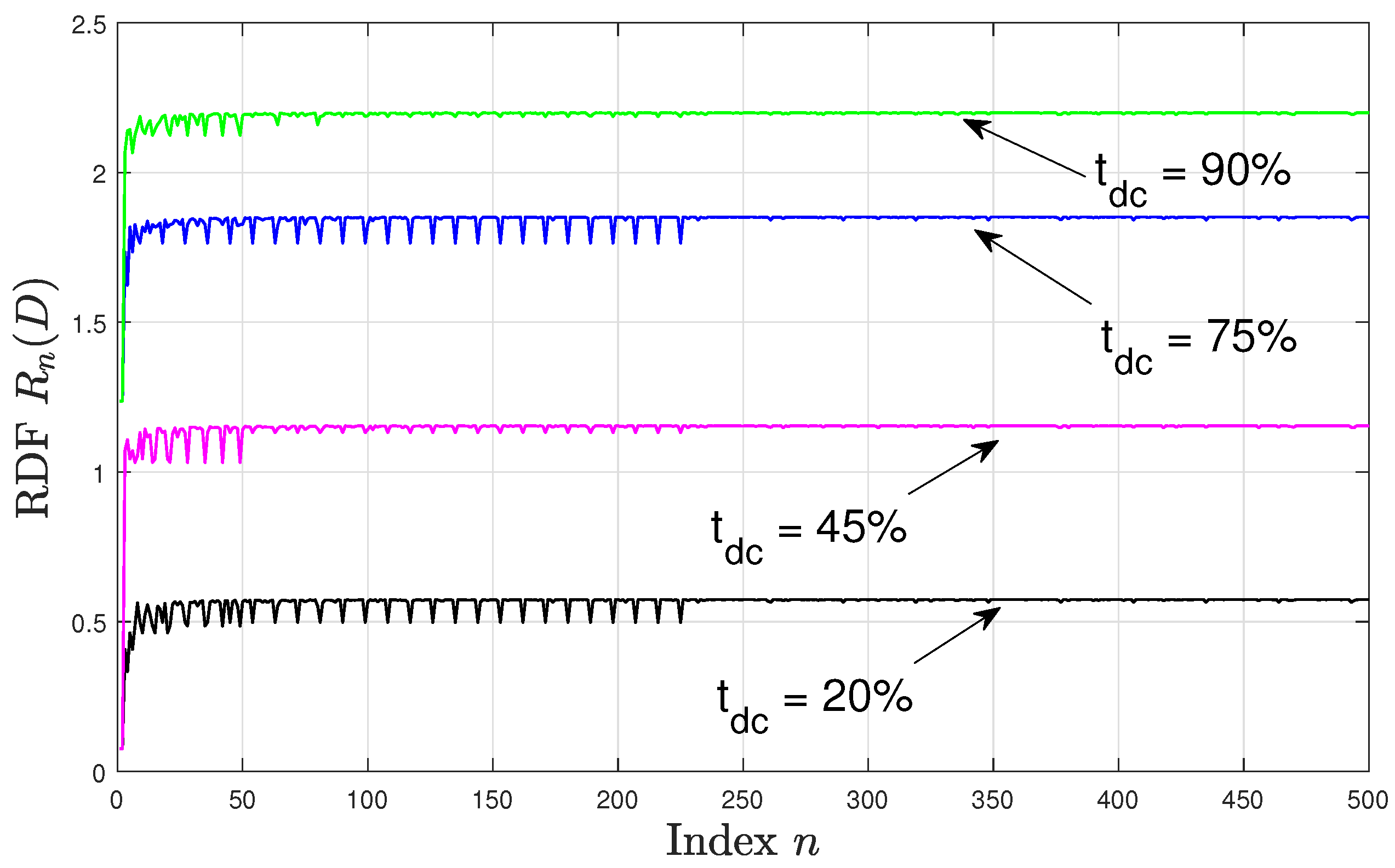
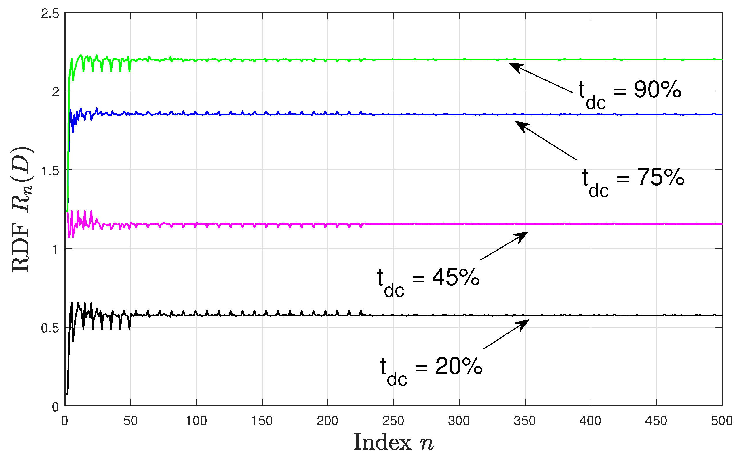
From Theorem 4 it follows that if the distortion satisfies $D<\underset{0\le t\le T_{\mathrm{ps}}}{min}{\sigma }_{S_{\mathrm{c}}}^2(t)$, the RDF of the asynchronously sampled CT WSCS Gaussian process is given by the limit superior of the sequence ${\{R_n(D)\}}_{n\in \mathcal{N}}$; where $R_n(D)$ is defined in Proposition 1. In this subsection, we study the sequence of RDFs ${\{R_n(D)\}}_{n\in \mathcal{N}}$ as n increases. For this evaluation setup, we fixed the distortion constraint at $D=0.18$ and set $ϵ=\frac{\pi }{7}$ and $p=2$. Let the variance of the CT WSCS Gaussian source process ${\sigma }_{S_{\mathrm{c}}}^2(t)$ be modelled by Equation (24) for two sampling time offsets $\varphi =\{0,\frac{1}{16}\}$. For each offset $\varphi$, four duty cycle values were considered: $t_{\mathrm{dc}}=[20,45,75,98]\%$. For each n we obtain the synchronous sampling mismatch ${ϵ}_n\triangleq \frac{\lfloor n·ϵ\rfloor }{n}$, which approaches $ϵ$ as $n\to \infty$, where $n\in \mathcal{N}$. Since ${ϵ}_n$ is a rational number, corresponding to a sampling period of $T_{\mathrm{s}}(n)=\frac{T_{\mathrm{ps}}}{p+{ϵ}_n}$, then for each n, the resulting dt process is WSCS with the period $p_n=p·n+\lfloor n·ϵ\rfloor$ and its RDF follows from Proposition 1.

Figure 2 and Figure 3 depict $R_n(D)$ for $n\in [1,500]$ with the specified duty cycles and sampling time offsets, where in Figure 2 there is no sampling time offset, i.e., $\varphi =0$, and in Figure 3 the sampling time offset is set to $\varphi =\frac{1}{16}$. We observe that in both figures the RDF values are higher for higher $t_{\mathrm{dc}}$. This can be explained by noting that for higher $t_{\mathrm{dc}}$ values, the resulting time-averaged variance of the DT source process increases, hence, a higher number of bits per source sample is required to encode the source process maintaining the same distortion value. Moreover, in all configurations, $R_n(D)$ varies significantly for smaller values of n. Comparing Figure 2 and Figure 3, we see that the pattern of these variations depends on the sampling time offset $\varphi$. For example, when $t_{\mathrm{dc}}=45\%$ at $n\in [4,15]$, then for $\varphi =0$ the rdf varies in the range $[1.032,1.143]$ bits per source sample, while for $\varphi =\frac{1}{16}$ the RDF varies in the range $[1.071,1.237]$ bits per source sample. However, as n increases above 230, the variations in $R_n(D)$ become smaller and are less dependent on the sampling time offset, and the resulting values of $R_n(D)$ are approximately in the same range for each $t_{\mathrm{dc}}$ in both Figure 2 and Figure 3 for $n\ge 230$. This behaviour can be explained by noting that as n varies, the period $p_n$ also varies and hence the statistics of the DT variance differs over its respective period. This consequently affects the resulting RDF (especially for small periods). As n increases ${ϵ}_n$ approaches the asynchronous sampling mismatch $ϵ$ and the period $p_n$ takes a sufficiently large value such that the samples of the DT variance over the period are identically distributed irrespective of the value of $\varphi$; leading to a negligible variation in the RDF as seen in the above figures.

5.2. The Variation of the RDF with the Sampling Rate

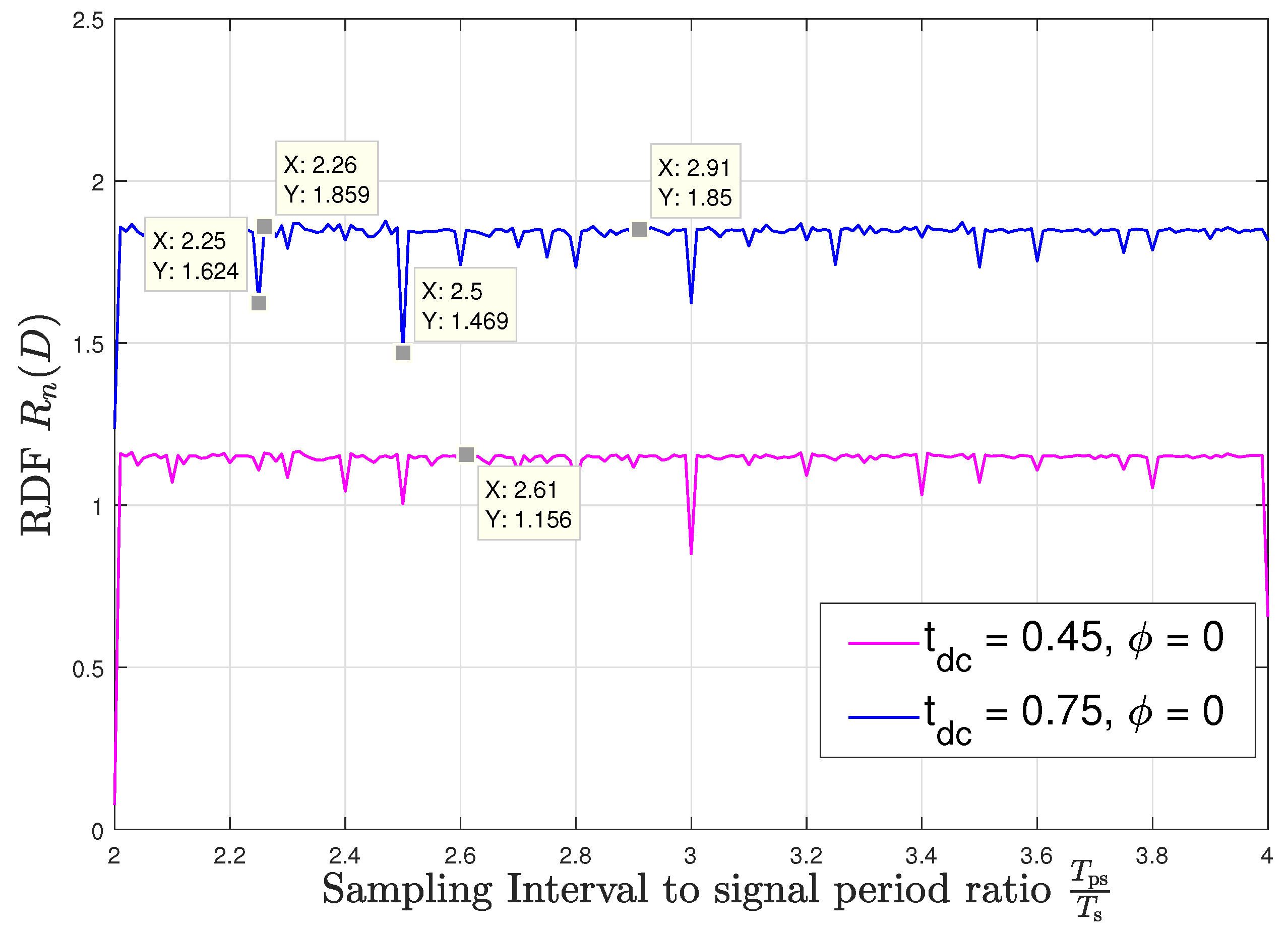
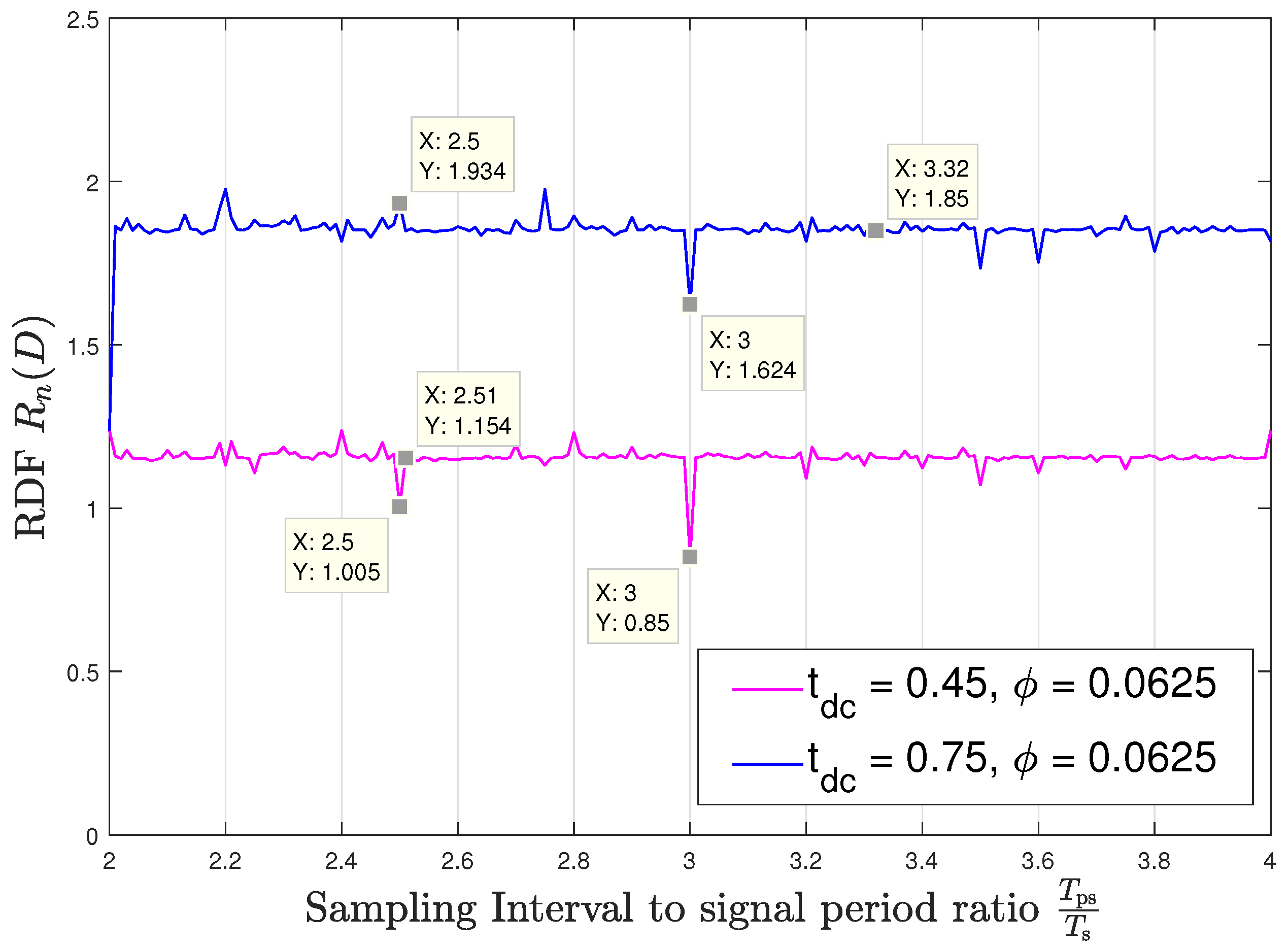
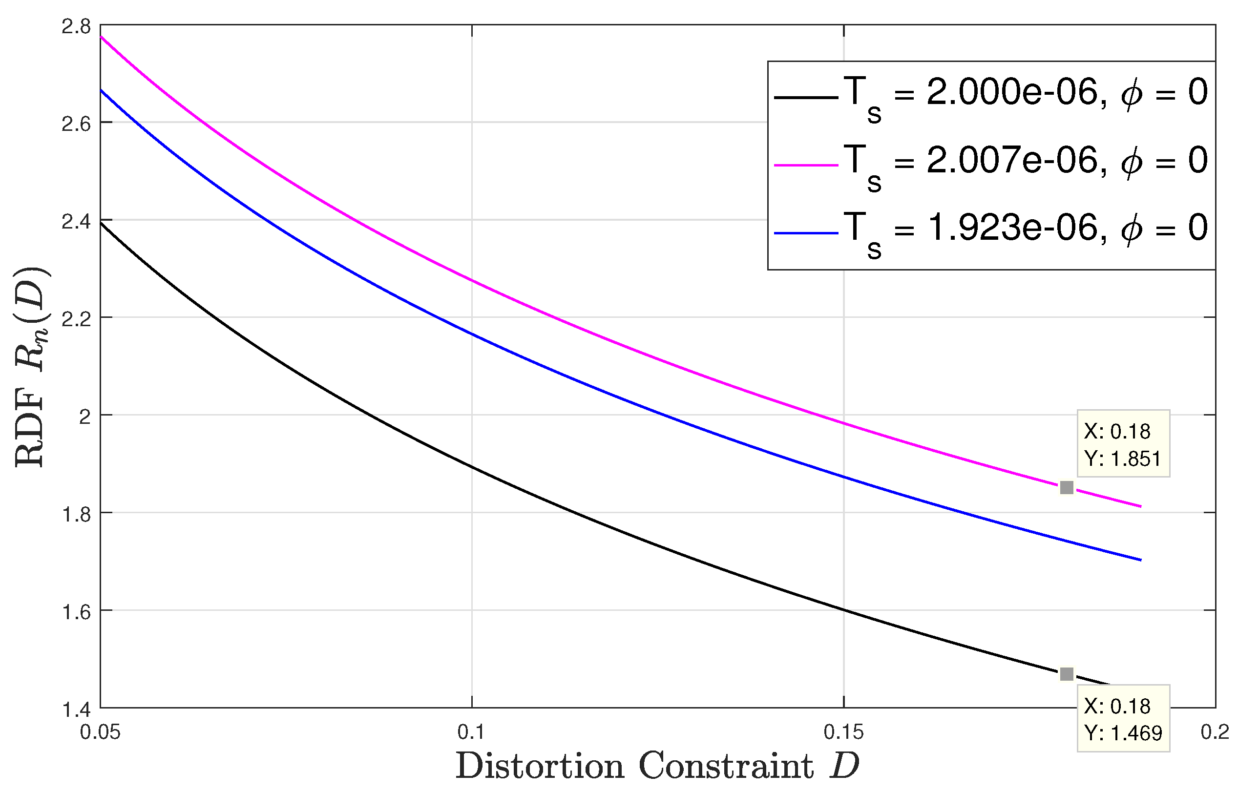
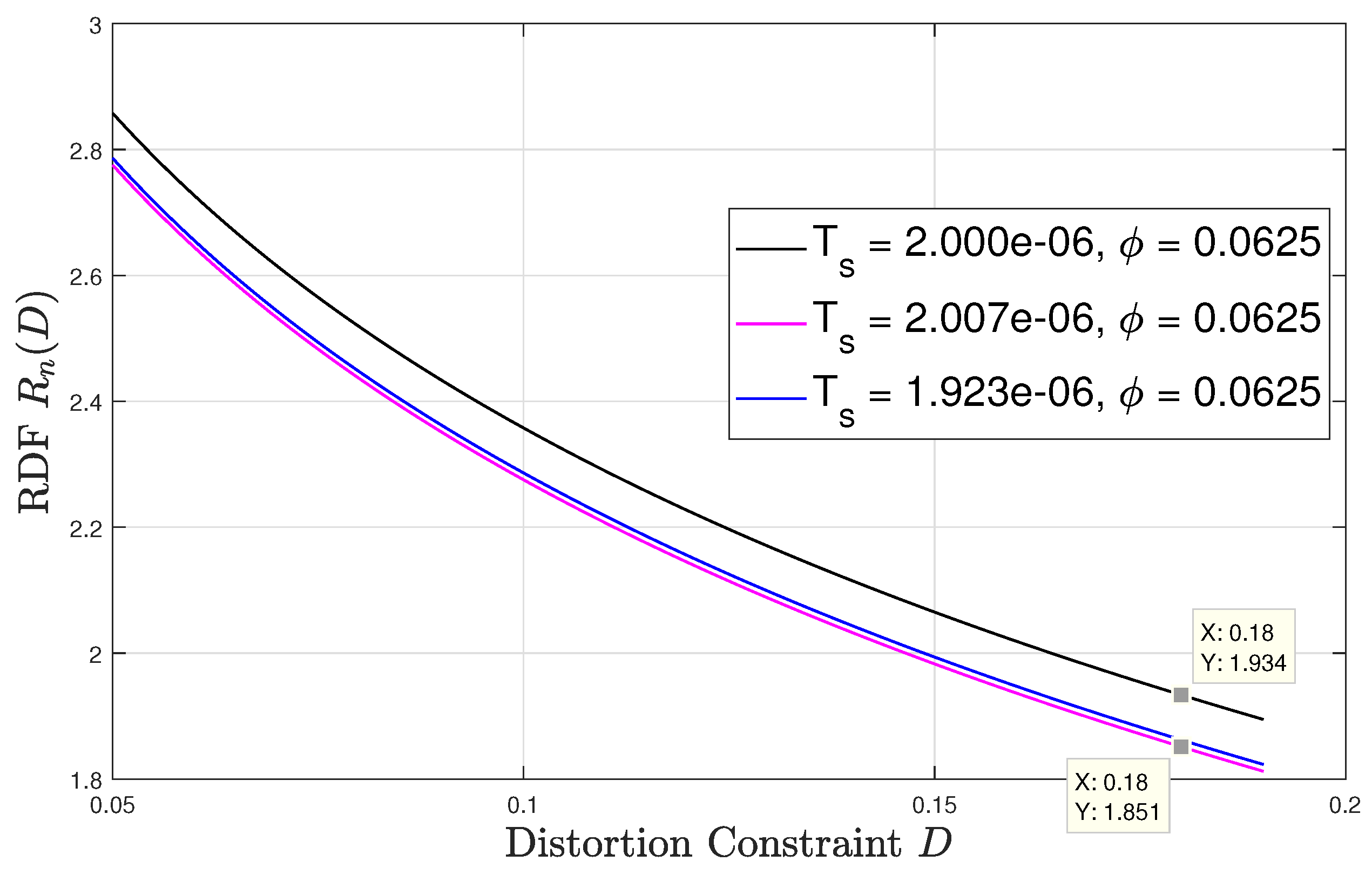
Next, we observe the dependence of the RDF for the sampled memoryless WSCS Gaussian process on the value of the sampling interval $T_{\mathrm{s}}$. For this setup, we fix the distortion constraint to $D=0.18$ and set the duty cycle in the source process (24) to $t_{\mathrm{dc}}=[45,75]\%$. Figure 4 and Figure 5 demonstrate the numerically evaluated values for $R_n(D)$ at sampling intervals in the range $2<\frac{T_{\mathrm{ps}}}{T_{\mathrm{s}}}<4$ with the sampling time offsets $\varphi =0$ and $\varphi =\frac{1}{16}$, respectively. We note that while the discussion which follows focuses on this range, as it corresponds to relatively low sampling rates—which are typically preferable in practice, the statements and observations regarding the relationship between the denominator of $\frac{T_{\mathrm{ps}}}{T_{\mathrm{s}}}$ and the value of $R_n(D)$, and regarding the continuity the RDF in the parameter $\frac{T_{\mathrm{ps}}}{T_{\mathrm{s}}}$, are directly applicable to any range of values of $\frac{T_{\mathrm{ps}}}{T_{\mathrm{s}}}$, e.g., when higher sampling rates are preferable. A very important insight which arises from the figures is that the sequence of RDFs $R_n(D)$ is not convergent; hence, for example, one cannot approach the RDF for $\frac{T_{\mathrm{ps}}}{T_{\mathrm{s}}}=2.5$ by simply taking rational values of $\frac{T_{\mathrm{ps}}}{T_{\mathrm{s}}}$ which approach $2.5$. This verifies that the RDF for asynchronous sampling cannot be obtained by straightforward application of previous results, and indeed, the entire analysis carried out in the manuscript is necessary for the desired characterization.

We observe in Figure 4 and Figure 5 that when $\frac{T_{\mathrm{ps}}}{T_{\mathrm{s}}}$ has a fractional part with a relatively small integer denominator, the variations in the RDF are significant and depend on the sampling time offset. These variations can either degrade the ability to accurately represent the source, which are the observed peaks in Figure 4 and Figure 5, or alternatively, allow to encode the signal to within the same distortion with smaller code rates, corresponding to the deeps in these figures. However, when $\frac{T_{\mathrm{ps}}}{T_{\mathrm{s}}}$ approaches an irrational number, the period of the sampled variance function becomes very long, and consequently, the RDF is approximately constant and independent of the sampling time offset. As an example, consider $\frac{T_{\mathrm{ps}}}{T_{\mathrm{s}}}=2.5$ and $t_{\mathrm{dc}}=75\%$: For sampling time offset $\varphi =0$ the rdf takes a value of $1.469$ bits per source sample, as shown in Figure 4 while for the offset of $\varphi =\frac{1}{16}$ the RDF peaks to $1.934$ bits per source sample as can be seen in Figure 5. On the other hand, when approaching asynchronous sampling, the RDF takes a nearly constant value of $1.85$ bits per source sample for all the considered values of $\frac{T_{\mathrm{ps}}}{T_{\mathrm{s}}}$ and this value is invariant to the offset $\varphi$. This follows since when the denominator of the fractional part of $\frac{T_{\mathrm{ps}}}{T_{\mathrm{s}}}$ increases, then the DT period of the resulting sampled variance, $p_n$, increases and practically captures the entire set of values of the CT variance regardless of the sampling time offset. In a similar manner as with the study on capacity in [17], we conjecture that since asynchronous sampling captures the entire set of values of the CT variance, the respective RDF represents the RDF of the analog source, which does not depend on the specific sampling rate and offset. Figure 4 and Figure 5 demonstrate how slight variations in the sampling rate can result in significant changes in the RDF. For instance, at $\varphi =0$ we observe in Figure 4 that when the sampling rate switches from $T_{\mathrm{s}}=2.25·T_{\mathrm{ps}}$ to $T_{\mathrm{s}}=2.26·T_{\mathrm{ps}}$, i.e., the sampling rate switches from being synchronous to being nearly asynchronous, then the RDF changes from $1.624$ bits per source sample to $1.859$ bits per source sample for $t_{\mathrm{dc}}=75\%$; also, we observe in Figure 5 for $t_{\mathrm{dc}}=45\%$, that when the sampling rate switches from $T_{\mathrm{s}}=2.5·T_{\mathrm{ps}}$ to $T_{\mathrm{s}}=2.51·T_{\mathrm{ps}}$, i.e., the sampling rate also switches from being synchronous to being nearly asynchronous, then the rdf changes from $1.005$ bits per source sample to $1.154$ bits per source sample.

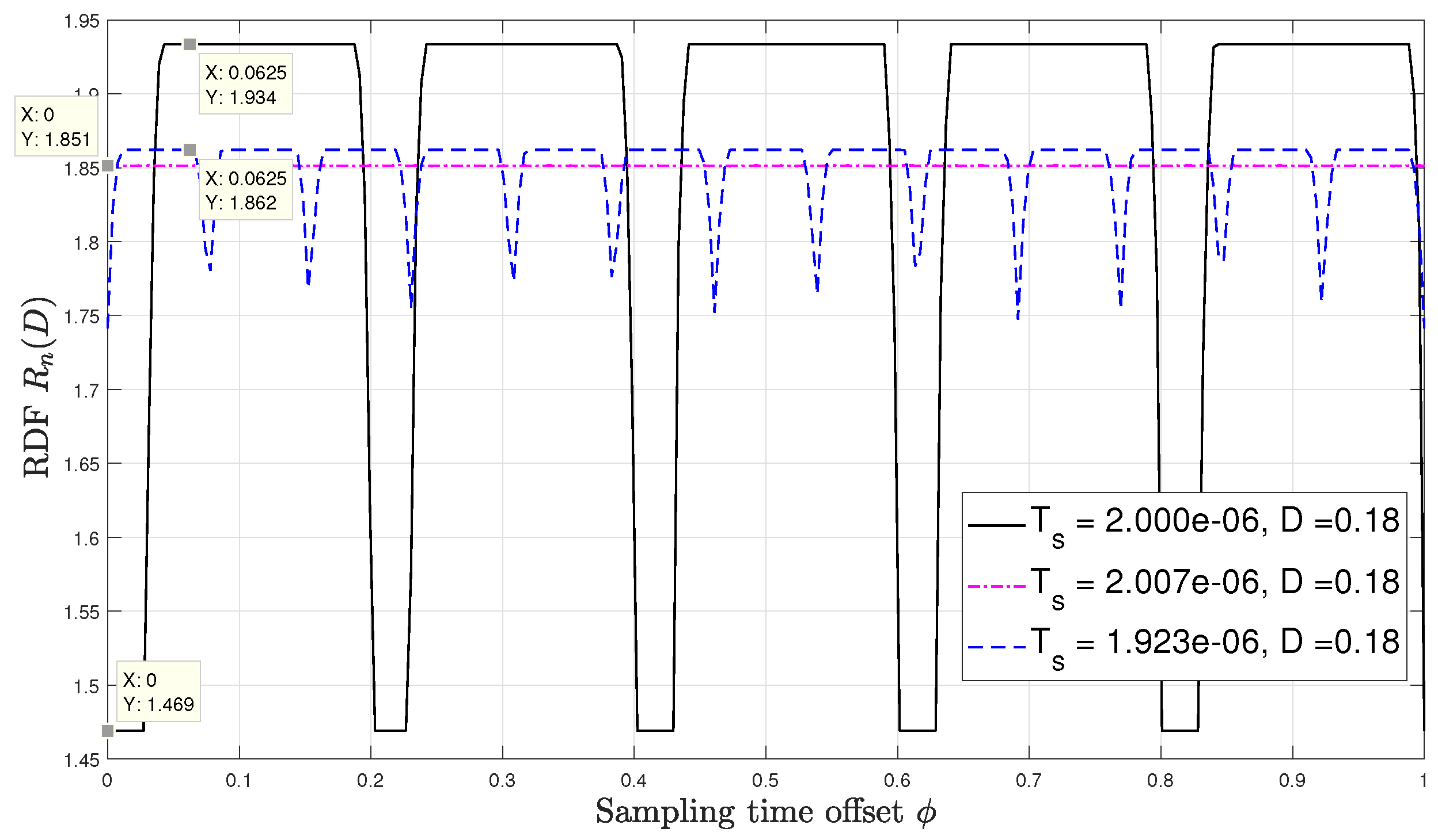
Lastly, Figure 6 and Figure 7 numerically evaluate the RDF versus the distortion constraint $D\in [0.05,0.19]$ for sampling time offsets of 0 and $\frac{1}{16}$ respectively. At each $\varphi$, the result is evaluated at three different values of synchronization mismatch $ϵ$. For this setup, we fix $t_{\mathrm{dc}}=75\%$, $p=2$ and $ϵ\in \{0.5,\frac{5\pi }{32},0.6\}$. The only mismatch value that refers to the asynchronous sampling case is $ϵ=\frac{5\pi }{32}$ and its corresponding sampling interval is approximately $2.007$ $\mathsf{\mu }$secs, which is a negligible variation from the sampling intervals corresponding to $ϵ\in \{0.5,0.6\}$, which are $2.000$ $\mathsf{\mu }$secs and $1.923$ $\mathsf{\mu }$secs, respectively. Observing both figures, we see that the rdf may vary significantly for very slight variation in the sampling rate. For instance, as shown in Figure 6 for $\varphi =0$, at $D=0.18$, a slight change in the synchronization mismatch from $ϵ=\frac{5\pi }{32}$ (i.e., $T_{\mathrm{s}}\approx 2.007\mathsf{\mu }$secs) to $ϵ=0.5$ (i.e., $T_{\mathrm{s}}=2.000\mathsf{\mu }$secs) results to approximately $20\%$ decrease in the rdf. For $\varphi =\frac{1}{16}$ the same change in the sampling synchronization mismatch at $D=0.18$ results in an increase in the RDF by roughly $4\%$. These results demonstrate the unique and counter-intuitive characteristics of the RDF of sampled WSCS signals which arise from our derivation. It is also interesting to examine how the RDF varies with the sampling time offset $\varphi$. To that aim we plot in Figure 8 the RDF vs. $\varphi$ for the three sampling rates used in Figure 6 and Figure 7 at $D=0.18$. The points marked on the plot correspond to $\varphi =0$ and $\varphi =\frac{1}{16}$ considered in Figure 6 and Figure 7, respectively. We observe that the RDF is indeed periodic with $\varphi$. These variations in the RDF occur as by changing $\varphi$ the number of high variance samples within a period of the variance of the DT process changes due to the duty cycle of the CT variance. Then, at $\varphi =0$ the periodic variance of the DT process corresponding to $T_{\mathrm{s}}=2.000\mathsf{\mu }\mathrm{secs}$ has the smallest number of high variance values within a period, and when $\varphi =\frac{1}{16}$ the periodic variance of the DT process corresponding to asynchronous sampling has the smallest number of high variance values within a period. For the asynchronous sampling rate the sampling time offset does not matter as in any case (nearly) all values of the CT variance are reflected in the variance of the DT process.

6. Conclusions

In this work the RDF of a sampled CT WSCS Gaussian source process was characterized for scenarios in which the resulting DT process is memoryless and the distortion is relatively small. This characterization shows the relationship between the sampling rate and the minimal number of bits per source sample required for compression at a given distortion. For cases in which the sampling rate is synchronized with the period of the statistics of the source process, the resulting DT process is WSCS and standard information theoretic framework can be used for deriving its RDF. For asynchronous sampling, information stability does not hold, and hence we resort to the information spectrum framework to obtain a characterization. To that aim we derived a relationship between some relevant information spectrum quantities for uniformly convergent sequences of RVs. This relationship was further applied to characterize the RDF of an asynchronously sampled CT WSCS Gaussian source process as the limit superior of a sequence of RDFs, each corresponding to the synchronous sampling of the CT WSCS Gaussian process. The results were derived in the low distortion regime, i.e., under the condition that the distortion constraint D is less than the minimum variance of the source, and for sampling intervals which are larger than the correlation length of the CT process. Our numerical examples give rise to non-intuitive insights which follow from the derivations. In particular, the numerical evaluation demonstrates that the RDF for a sampled CT WSCS Gaussian source can change dramatically with minor variations in the sampling rate and the sampling time offset. In particular, when the sampling rate switches from being synchronous to being asynchronous and vice versa, the RDF may change considerably as the statistical model of the source switches between WSCS and WSACS. The resulting analysis enables determining the sampling system parameters in order to facilitate accurate and efficient source coding of acquired CT signals.

References

- Gardner, W.; Brown, W.; Chen, C.K. Spectral correlation of modulated signals: Part II-digital modulation. IEEE Trans. Commun. 1987, 35, 595–601. [Google Scholar] [CrossRef]
- Giannakis, G.B. Cyclostationary signal analysis. In Digital Signal Processing Handbook; CRC PRESS: Boca Raton, FL, USA, 1998; pp. 17–21. [Google Scholar]
- Gardner, W.A.; Napolitano, A.; Paura, L. Cyclostationarity: Half a century of research. Signal Process. 2006, 86, 639–697. [Google Scholar] [CrossRef]
- Berger, T.; Gibson, J.D. Lossy source coding. IEEE Trans. Inf. Theory 1998, 44, 2693–2723. [Google Scholar] [CrossRef] [Green Version]
- Cover, T.M.; Thomas, J.A. Elements of Information Theory; John Wiley & Sons: New York, NY, USA, 2006. [Google Scholar]
- Wolf, J.K.; Wyner, A.D.; Ziv, J. Source coding for multiple descriptions. Bell Syst. Tech. J. 1980, 59, 1417–1426. [Google Scholar] [CrossRef]
- Wyner, A.D.; Ziv, J. The rate-distortion function for source coding with side information at the decoder. IEEE Trans. Inf. Theory 1976, 22, 1–10. [Google Scholar] [CrossRef]
- Oohama, Y. Gaussian multiterminal source coding. IEEE Trans. Inf. Theory 1997, 43, 1912–1923. [Google Scholar] [CrossRef]
- Pandya, A.; Kansal, A.; Pottie, G.; Srivastava, M. Lossy source coding of multiple Gaussian sources: m-helper problem. In Proceedings of the IEEE Information Theory Workshop, San Antonio, TX, USA, 24–29 October 2004; pp. 34–38. [Google Scholar]
- Gallager, R.G. Information Theory and Reliable Communication; Springer: Berlin, Germany, 1968; Volume 588. [Google Scholar]
- Harrison, M.T. The generalized asymptotic equipartition property: Necessary and sufficient conditions. IEEE Trans. Inf. Theory 2008, 54, 3211–3216. [Google Scholar] [CrossRef] [Green Version]
- Kipnis, A.; Goldsmith, A.J.; Eldar, Y.C. The distortion rate function of cyclostationary Gaussian processes. IEEE Trans. Inf. Theory 2018, 64, 3810–3824. [Google Scholar] [CrossRef] [Green Version]
- Napolitano, A. Cyclostationarity: New trends and applications. Signal Process. 2016, 120, 385–408. [Google Scholar] [CrossRef]
- Han, T.S. Information-Spectrum Methods in Information Theory; Springer: Berlin, Germany, 2003; Volume 50. [Google Scholar]
- Verdú, S.; Han, T.S. A general formula for channel capacity. IEEE Trans. Inf. Theory 1994, 40, 1147–1157. [Google Scholar] [CrossRef] [Green Version]
- Zeng, W.; Mitran, P.; Kavcic, A. On the information stability of channels with timing errors. In Proceedings of the IEEE International Symposium on Information Theory (ISIT), Seattle, WA, USA, 9–14 July 2006; pp. 1885–1889. [Google Scholar]
- Shlezinger, N.; Abakasanga, E.; Dabora, R.; Eldar, Y.C. The Capacity of Memoryless Channels with Sampled Cyclostationary Gaussian Noise. IEEE Trans. Commun. 2020, 68, 106–121. [Google Scholar] [CrossRef]
- Shannon, C.E. Communication in the presence of noise. Proc. IEEE 1998, 86, 447–457. [Google Scholar] [CrossRef]
- Cherif, F. A various types of almost periodic functions on Banach spaces: Part I. Int. Math. Forum 2011, 6, 921–952. [Google Scholar]
- Shlezinger, N.; Dabora, R. On the capacity of narrowband PLC channels. IEEE Trans. Commun. 2015, 63, 1191–1201. [Google Scholar] [CrossRef] [Green Version]
- Shlezinger, N.; Dabora, R. The capacity of discrete-time Gaussian MIMO channels with periodic characteristics. In Proceedings of the IEEE International Symposium on Information Theory (ISIT), Barcelona, Spain, 10–16 October 2016; pp. 1058–1062. [Google Scholar]
- Shlezinger, N.; Zahavi, D.; Murin, Y.; Dabora, R. The secrecy capacity of Gaussian MIMO channels with finite memory. IEEE Trans. Inf. Theory 2017, 63, 1874–1897. [Google Scholar] [CrossRef]
- Heath, R.W.; Giannakis, G.B. Exploiting input cyclostationarity for blind channel identification in OFDM systems. IEEE Trans. Signal Process. 1999, 47, 848–856. [Google Scholar] [CrossRef] [Green Version]
- Shaked, R.; Shlezinger, N.; Dabora, R. Joint estimation of carrier frequency offset and channel impulse response for linear periodic channels. IEEE Trans. Commun. 2017, 66, 302–319. [Google Scholar] [CrossRef]
- Shlezinger, N.; Dabora, R. Frequency-shift filtering for OFDM signal recovery in narrowband power line communications. IEEE Trans. Commun. 2014, 62, 1283–1295. [Google Scholar] [CrossRef] [Green Version]
- El Gamal, A.; Kim, Y.H. Network Information Theory; Cambridge University Press: Cambridge, UK, 2011. [Google Scholar]
- Wu, X.; Xie, L.L. On the optimal compressions in the compress-and-forward relay schemes. IEEE Trans. Inf. Theory 2013, 59, 2613–2628. [Google Scholar] [CrossRef] [Green Version]
- Zitkovic, G. Lecture Notes on the Theory of Probability Parts I and II. Available online: https://web.ma.utexas.edu/users/gordanz/lecture_notes_page.html (accessed on 12 March 2020).
- Papoulis, A. Probability, Random Variables, and Stochastic Processes; McGraw-Hill: New York, NY, USA, 2002. [Google Scholar]
- Zamir, R.; Kochman, Y.; Erez, U. Achieving the Gaussian rate–distortion function by prediction. IEEE Trans. Inf. Theory 2008, 54, 3354–3364. [Google Scholar] [CrossRef]
- Rudin, W. Principles of Mathematical Analysis; International series in pure and applied mathematics; McGraw-Hill: New York, NY, USA, 1976. [Google Scholar]
- Dixmier, J. General Topology; Springer: New York, NY, USA, 1984. [Google Scholar]
- Stein, E.M.; Shakarchi, R. Real Analysis: Measure Theory, Integration, and Hilbert Spaces; Princeton University Press: Princeton, NJ, USA, 2009. [Google Scholar]
- Kolmogorov, A. On the Shannon theory of information transmission in the case of continuous signals. IRE Trans. Inf. Theory 1956, 2, 102–108. [Google Scholar] [CrossRef]
- Scheffé, H. A useful convergence theorem for probability distributions. Ann. Math. Stat. 1947, 18, 434–438. [Google Scholar] [CrossRef]
- Bromiley, P. Products and convolutions of Gaussian probability density functions. Tina-Vision Memo 2003, 3, 1. [Google Scholar]
- Kosorok, M.R. Introduction to Empirical Processes and Semiparametric Inference.; Springer: New York, NY, USA, 2008. [Google Scholar]
- Williams, D. Probability with Martingales; Cambridge University Press: Cambridge, UK, 1991. [Google Scholar]
- Dobrushin, R.L. A general formulation of the fundamental theorem of Shannon in the theory of information. Uspekhi Matematicheskikh Nauk 1959, 14, 3–104. [Google Scholar]
- Billingsley, P. Convergence of Probability Measures; John Wiley & Sons: New York, NY, USA, 2013. [Google Scholar]
- Venkataramanan, R.; Pradhan, S.S. Source coding with feed-forward: Rate-distortion theorems and error exponents for a general source. IEEE Trans. Inf. Theory 2007, 53, 2154–2179. [Google Scholar] [CrossRef]
Figure 1.
Source coding block diagram.
Figure 2.
versus n; offset .
Figure 3.
Figure 4.
versus ; offset .
Figure 5.
Figure 6.
versus D; offset .
Figure 7.
Figure 8.
versus at .
© 2020 by the authors. Licensee MDPI, Basel, Switzerland. This article is an open access article distributed under the terms and conditions of the Creative Commons Attribution (CC BY) license (http://creativecommons.org/licenses/by/4.0/).
Share and Cite
MDPI and ACS Style
Abakasanga, E.; Shlezinger, N.; Dabora, R. On the Rate-Distortion Function of Sampled Cyclostationary Gaussian Processes. Entropy 2020, 22, 345. https://0-doi-org.brum.beds.ac.uk/10.3390/e22030345
AMA Style
Abakasanga E, Shlezinger N, Dabora R. On the Rate-Distortion Function of Sampled Cyclostationary Gaussian Processes. Entropy. 2020; 22(3):345. https://0-doi-org.brum.beds.ac.uk/10.3390/e22030345
Chicago/Turabian StyleAbakasanga, Emeka, Nir Shlezinger, and Ron Dabora. 2020. "On the Rate-Distortion Function of Sampled Cyclostationary Gaussian Processes" Entropy 22, no. 3: 345. https://0-doi-org.brum.beds.ac.uk/10.3390/e22030345
Note that from the first issue of 2016, this journal uses article numbers instead of page numbers. See further details here.