Optimizing Age Penalty in Time-Varying Networks with Markovian and Error-Prone Channel State

Abstract

In this paper, we consider a scenario where the base station (BS) collects time-sensitive data from multiple sensors through time-varying and error-prone channels. We characterize the data freshness at the terminal end through a class of monotone increasing functions related to Age of information (AoI). Our goal is to design an optimal policy to minimize the average age penalty of all sensors in infinite horizon under bandwidth and power constraint. By formulating the scheduling problem into a constrained Markov decision process (CMDP), we reveal the threshold structure for the optimal policy and approximate the optimal decision by solving a truncated linear programming (LP). Finally, a bandwidth-truncated policy is proposed to satisfy both power and bandwidth constraint. Through theoretical analysis and numerical simulations, we prove the proposed policy is asymptotic optimal in the large sensor regime.

1. Introduction

The requirements for data freshness in numerous emerging applications are becoming stricter [1,2]. However, the limited resources and bandwidth, together with the fading and error-prone channel characteristics, prevent the control terminal from obtaining the newest information. Moreover, the traditional optimization goals like low delay and high throughput cannot fully characterize the requirement of data freshness. Therefore, it is necessary to introduce new metrics to capture data freshness in such systems and design strategies to optimize the system performance in the presence of resource and environment restrictions.

Recently, a popular metric, Age of information (AoI), has been proposed in [3] to measure the data freshness. Since then, the optimization of age performance under different systems has been a research hotspot. The simple point-to-point system model has been studied in [3,4,5,6,7,8,9,10,11]. When update packets are generated by external sources and are queued in a buffer before transmission, queuing theory can be used to analyze the performance of such system, see, e.g., in, [3,4,5,6,7,8]. In [3], it is shown that the optimum packet generation rate of a first-come-first-served (FCFS) system should achieve a trade-off between throughput and delay. In [8], dynamic pricing is used as an incentive to balance the AoI evolution and the monetary payments to the users. Other studies [9,10,11] consider the generate-at-will system without a queue. Energy constraints are studied in [10,11] to find the trade-off between the age performance and energy consumption. In [11], both offline and online heuristic policies are proposed to optimize the average AoI, which outperform the greedy approach.

Apart from the point-to-point systems, scheduling strategies in the multi-user networks are studied in [12,13,14,15,16,17,18,19]. Different scheduling policies are studied in [12] to minimize the average AoI performance through unreliable channels, and Maatouk et al. verify the asymptotic optimality of Whittle’s index policy by setting an upper bound on the maximum AoI [13]. When each user has a minimum throughput requirement, the authors of [14] propose the Drift-Plus-Penalty policy using Lyapunov analysis to minimize the average AoI performance. In [17], a slotted ALOHA algorithm is proposed to minimize the average AoI, whose performance is verified in the large system regime.

Notice that in many general scenarios, like remote estimation [20,21], the proper evaluation of data freshness is a function of AoI instead of AoI itself. Therefore, the metric of Cost of Update Delay (CoUD) in [7] and age penalty function in [9] have been proposed to measure data freshness in a general setting. However, those works focus on minimizing data freshness in a single-user network, and the multi-user model is rarely considered. To fill this gap, we study a scenario where the base station (BS) collects time-sensitive data from multiple sensors through time-varying channels. We generalize our previous work [22] by considering a more realistic time-varying channel with packet loss and a more general age penalty measurement to model different application scenarios. The main contributions of the paper are listed as follows.

• We study the scheduling strategy for age penalty minimization in multi-sensor bandwidth constrained networks through time-varying and error-prone channel links with power limited sensors. To study a practical network, we model the channel to be a finite-state ergodic Markov chain. The packet loss probability and power consumption depend on the current channel state. Unlike previous work, we model the effect of data staleness in different scenarios via a class of monotone increasing function related to AoI.
• Through relaxing the hard bandwidth constraint and Lagrange multipliers, we decouple the multi-sensor optimization problem into several single-sensor constrained Markov decision process (CMDP) problems. To deal with the potential infinite age penalty, we deduce the threshold structure of the optimal policy and then obtain the approximate optimal single-sensor scheduling decision by solving a truncated linear programming (LP). We prove the solution to the LP is asymptotic optimal when the truncated threshold is sufficiently large.
• The sub-gradient ascend method is applied to find the optimal Lagrange multiplier to satisfy the relaxed bandwidth constraint. Finally, we propose the truncated stationary policy to meet the hard bandwidth constraint. The average performance of the strategy is verified through theoretical analysis and numerical simulations.

The remainder of this paper is organized as follows. The network model, the AoI metric, and the age penalty function are introduced in Section 2. In Section 3, we formulate the primal scheduling problem, and then decouple it into independent single-sensor problems through bandwidth relaxation and Lagrange multipliers. The approximate optimal policy for single-sensor problem is obtained in Section 4 by solving an LP. In Section 5, the asymptotic optimal truncated policy is proposed. Finally, Section 6 provides simulation results to verify the performance of the proposed truncated policy, and Section 7 draws the conclusion.

Notations: All the vectors and matrices are denoted in boldface. The probability of $\mathcal{A}$ given $\mathcal{B}$ is denoted as $\mathrm{Pr}\left(\mathcal{A}\right|\mathcal{B})$. Let ${\mathbb{E}}_{\pi }\left[X\right]$ be the expectation of variable X given $\pi$. The cardinality of a set $\mathsf{\Omega }$ is written as $\left|\mathsf{\Omega }\right|$.

2. System Model

2.1. Network Model

In this work, we consider a BS collecting update packets from N time-sensitive sensors through time-varying channels. The time is slotted, and $t\in \{1,2,...,T\}$ is used to denote the current slot index. Define $u_n\left(t\right)$ to be the scheduling decision for sensor n in slot t, where $u_n\left(t\right)=1$ means the sensor n chooses to send the newest packet, while $u_n\left(t\right)=0$ means idling the channel link. Assume all the scheduling behaviors take place at the beginning of each slot and the packet transmission delay through all the channel links is one slot. Due to the limited bandwidth capacity of the BS, the total number of sensors to be scheduled in one slot cannot be larger than M. Here, we assume $M<N$ so that the problem is nontrivial:

$$\sum _{n=1}^N{u}_n\left(t\right)\le M,\forall t.$$

(1)

To model the time varying effect, we assume that the channel link connecting the BS and each sensor n is an ergodic Q-state Markov chain. Denote $q_n\left(t\right)\in \{1,2,\cdots ,Q\}$ to be the channel state of link n in slot t. Without loss of generality, we assume that the channel state becomes more noisy as the state index becomes larger. Denote $P_n=\left\{p_{ij}^n\right\}$ to be the Markov state transition matrix of link n, and the entry $p_{ij}^n$ means the probability of changing into state j in the next slot given the current state i, i.e.,

$$p_{ij}^n\triangleq \mathrm{Pr}\{q_n(t+1)=j|q_n\left(t\right)=i\}.$$

(2)

Due to different channel states, the sensors should use different energy for both saving energy and successful decoding of the packet at the receiver. We denote $w\left(q\right)$ to be the energy consumption for scheduling when the channel state is q. Notice that the energy consumption tends to be larger as the channel state becomes more noisy to combat the channel fading, i.e., $w\left(1\right)<w\left(2\right)<...<w\left(Q\right)$. Besides, due to the power limit of each sensor n, the total average power consumption cannot exceed the upper bound, denoted by ${\mathcal{E}}_n$, i.e.,

$$\underset{T\to \infty }{lim}\frac{1}{T}{\mathbb{E}}_{\pi }\left[\sum _{t=1}^T{u}_n\left(t\right)w\left(q_n\left(t\right)\right)\right]\le {\mathcal{E}}_n,\forall n,$$

(3)

where $\pi$ is a scheduling policy.

Given channel state q, we assume that there exists the probability of packet loss ${\epsilon }_{n,q}$ through link n due to decoding error or inaccurate estimation.

2.2. Age of Information and Age Penalty

In the network described above, the BS wishes to obtain the freshest information for further process or accurate prediction. We model the data staleness at the terminal end as a monotone increasing age penalty function $f(·)$ of Age of information (AoI). By definition, AoI is the difference between the current time slot and the time slot that the freshest data received by the BS is generated by the sensor [3].

Let $x_n\left(t\right)$ be the AoI of sensor n in slot t. According to the definition, if the sensor is scheduled in slot t and there is no packet loss, then $x_n(t+1)=1$; otherwise, $x_n(t+1)=x_n\left(t\right)+1$. In conclusion, the AoI evolves as follows,

$$\begin{array}{c}\mathrm{Pr}(x_n(t+1)=x^{\prime }|x_n\left(t\right)=x,u_n\left(t\right)=u)=\left\{\begin{array}{cc}1-{\epsilon }_{n,q_n\left(t\right)},\hfill & x^{\prime }=1,u=1;\hfill \\ {\epsilon }_{n,q_n\left(t\right)},\hfill & x^{\prime }=x+1,u=1;\hfill \\ 1,\hfill & x^{\prime }=x+1,u=0;\hfill \\ 0,\hfill & \mathrm{otherwise}.\hfill \end{array}\right.\end{array}$$

(4)

3. Problem Formulation and Decomposition

3.1. Problem Formulation

For given network, we measure the data freshness at the terminal side by computing the average age penalty under scheduling policy $\pi$, denoted by $J\left(\pi \right)$, i.e.,

$$J\left(\pi \right)=\underset{T\to \infty }{lim}\frac{1}{NT}{\mathbb{E}}_{\pi }\left[\sum _{t=1}^T\sum _{n=1}^{N}f\left(x_n\left(t\right)\right)|\mathit{x}\left(0\right)\right],$$

(5)

where $\mathit{x}\left(0\right)=[x_1\left(0\right),x_2\left(0\right),...,x_N\left(0\right)]$ states the initial AoI of the system. In this work, we assume that the system is synchronized with all the sensors at the beginning, i.e., $x_n\left(0\right)=1,\forall n$, and thus omit $\mathit{x}\left(0\right)$ in the further analysis.

We denote ${\mathsf{\Pi }}_{\mathit{CP}}$ to be the set of all possible causal policies whose decisions are only based on current and historic information while satisfying both bandwidth and power constraints. Then, our goal is to optimize Equation (5) by choosing a scheduling policy $\pi \in {\mathsf{\Pi }}_{\mathit{CP}}$. Therefore, the primal optimization problem can be written as

Problem 1

(Primal Scheduling Problem).

$$\underset{\pi \in {\mathsf{\Pi }}_{\mathit{CP}}}{min}\underset{T\to \infty }{lim}\frac{1}{NT}{\mathbb{E}}_{\pi }\left[\sum _{n=1}^N\sum _{t=1}^{T}f\left(x_n\left(t\right)\right)\right],$$

(6a)

$$\begin{array}{cc}\hfill s.t.& \sum _{n=1}^N{u}_n\left(t\right)\le M,\forall t,\hfill \end{array}$$

(6b)

$$\begin{array}{cc}\hfill & \underset{T\to \infty }{lim}\frac{1}{T}{\mathbb{E}}_{\pi }\left[\sum _{t=1}^T{u}_n\left(t\right)w\left(q_n\left(t\right)\right)\right]\le {\mathcal{E}}_n,\forall n.\hfill \end{array}$$

(6c)

3.2. Problem Decomposition

Notice that Equation (6b) is an integer programming where the exponential growth rate of state and action space set obstacles in solving Problem 1. Therefore, we formulate a relaxed version of Problem 1, where the primal bandwidth constraint in every slot is replaced by a time-average bandwidth constraint. We will then show that the relaxed problem can be solved by sensor level decoupling, which greatly reduces the cardinality of the state and action space.

Problem 2

(Relaxed Primal Scheduling Problem).

$$Ag{e}_R^{*}=\underset{\pi \in {\mathsf{\Pi }}_{\mathit{CP}}}{min}\underset{T\to \infty }{lim}\frac{1}{NT}{\mathbb{E}}_{\pi }\left[\sum _{n=1}^N\sum _{t=1}^{T}f\left(x_n\left(t\right)\right)\right],$$

(7a)

$$\begin{array}{cc}\hfill s.t.& \underset{T\to \infty }{lim}\frac{1}{T}{\mathbb{E}}_{\pi }\left[\sum _{t=1}^T\sum _{n=1}^N{u}_n\left(t\right)\right]\le M,\hfill \end{array}$$

(7b)

$$\begin{array}{cc}\hfill & \underset{T\to \infty }{lim}\frac{1}{T}{\mathbb{E}}_{\pi }\left[\sum _{t=1}^T{u}_n\left(t\right)w\left(q_n\left(t\right)\right)\right]\le {\mathcal{E}}_n,\forall n.\hfill \end{array}$$

(7c)

Denote ${\pi }_R^{*}$ to be the optimal policy of Problem 2. The following theorem ensures that the optimal policy of the relaxed problem is composed of several local optimal policies ${\pi }_n^{*}$, each of which depends on its own channel state and AoI evolution regardless of others.

Theorem 1.

The optimal policy of Problem 2 can be decoupled into local optimal policies, i.e., ${\pi }_R^{*}={\pi }_1^{*}\otimes {\pi }_2^{*}\otimes \cdots \otimes {\pi }_N^{*}$. Each of the local policy ${\pi }_n^{*}$ has the following properties.

$$\begin{array}{cc}\hfill & Ag{e}_R^{*}=\underset{T\to \infty }{lim}\frac{1}{NT}\sum _{t=1}^T\sum _{n=1}^N{\mathbb{E}}_{{\pi }_n^{*}}\left[f\left(x_n\left(t\right)\right)\right],\hfill \\ \hfill & \underset{T\to \infty }{lim}\frac{1}{T}\sum _{t=1}^T\sum _{n=1}^N{\mathbb{E}}_{{\pi }_n^{*}}\left[u_n\left(t\right)\right]\le M,\hfill \\ \hfill & \underset{T\to \infty }{lim}\frac{1}{T}{\mathbb{E}}_{{\pi }_n^{*}}\left[\sum _{t=1}^T{u}_n\left(t\right)w\left(q_n\left(t\right)\right)\right]\le {\mathcal{E}}_n,\forall n.\hfill \end{array}$$

The proof of Theorem 1 is provided in Appendix A.

In order to find the local optimal polices, we introduce a Lagrange multiplier $\lambda \ge 0$ to eliminate the relaxed bandwidth constraint, and the Lagrange function is as follows,

$$\begin{array}{c}\hfill \mathcal{L}(\pi ,\lambda )=\underset{T\to \infty }{lim}\frac{1}{NT}\sum _{n=1}^N\sum _{t=1}^T{\mathbb{E}}_{{\pi }_n}\left[f\left(x_n\left(t\right)\right)+\lambda u_n\left(t\right)-\lambda \frac{M}{N}\right],\end{array}$$

where the Lagrange multiplier $\lambda$ can be seen as a scheduling penalty which will increase the function value if there are more than M sensors to be scheduled per slot in average.

For fixed $\lambda$, we can now further decouple the relaxed scheduling problem into N single-sensor cross-layer designs, each of which has the corresponding power constraint in Equation (7c):

Problem 3

(Single-Sensor Decoupled Problem).

$$\underset{{\pi }_n\in {\mathsf{\Pi }}_{\mathit{CP}}}{min}\underset{T\to \infty }{lim}\frac{1}{T}{\mathbb{E}}_{{\pi }_n}\left[\sum _{t=1}^T\left(f\left(x_n\left(t\right)\right)+\lambda u_n\left(t\right)\right)\right],$$

(8a)

$$\begin{array}{cc}\hfill s.t.& \underset{T\to \infty }{lim}\frac{1}{T}{\mathbb{E}}_{{\pi }_n}\left[\sum _{t=1}^T{u}_n\left(t\right)w\left(q_n\left(t\right)\right)\right]\le {\mathcal{E}}_n.\hfill \end{array}$$

(8b)

As the resolution of each decoupled problem is independent of n, we omit the subscript n in further analysis.

4. Single-Sensor Problem Resolution

4.1. Constrained Markov Decision Process Formulation

First, we notice that the decoupled problem is a constrained Markov decision process of which the elements $(\mathbb{S},\mathbb{A},\mathrm{Pr}(·|·),c(·))$ and constraint are explained as follows.

• State Space: The state of each sensor consists of two parts: the current AoI $x\left(t\right)$ and channel state $q\left(t\right)$. Thus, $\mathbb{S}=\{x\times q\}$ is infinite but countable.
• Action Space: There are two possible actions in the action space $\mathbb{A}$ for the scheduling policy, denoted by $u\left(t\right)$. Action $u\left(t\right)=1$ means the sensor chooses to schedule while $u\left(t\right)=0$ means idling. Notice that here $u\left(t\right)$ does not need to satisfy the bandwidth constraint.
• Probability Transition Function: According to Equations (2) and (4), the probability transition function can be written out as follows.

  $$\begin{array}{cc}\hfill & \mathrm{Pr}\left((x+1,q^{\prime })\right|(x,q),u=0)=p_{q{q}^{\prime }},\hfill \\ \hfill & \mathrm{Pr}\left((x+1,q^{\prime })\right|(x,q),u=1)=p_{q{q}^{\prime }}{\epsilon }_{n,q},\hfill \\ \hfill & \mathrm{Pr}\left((1,q^{\prime })\right|(x,q),u=1)=p_{q{q}^{\prime }}(1-{\epsilon }_{n,q}).\hfill \end{array}$$
• One-Step Cost: The one-step cost consists of two parts: the age penalty growth and scheduling penalty, which can be computed by

  $$c_x(x\left(t\right),q\left(t\right),u\left(t\right))=f\left(x\left(t\right)\right)+\lambda u\left(t\right).$$

  (9)
  And the one-step power consumption is

  $$c_E(x\left(t\right),q\left(t\right),u\left(t\right))=u\left(t\right)w\left(q\left(t\right)\right).$$

  (10)

Now our goal is to optimize the following average one-step cost,

$$\underset{\pi \in {\mathsf{\Pi }}_{\mathit{CP}}}{min}\underset{T\to \infty }{lim}\frac{1}{T}{\mathbb{E}}_{\pi }\left[\sum _{t=1}^T{c}_x(x\left(t\right),q\left(t\right),u\left(t\right))\right],$$

(11)

under the following average power constraint,

$$\underset{T\to \infty }{lim}\frac{1}{T}{\mathbb{E}}_{\pi }\left[\sum _{t=1}^T{c}_E(x\left(t\right),q\left(t\right),u\left(t\right))\right]\le \mathcal{E}.$$

(12)

4.2. Characterization of the Optimal Policy

To search for the stationary optimal policy, we can further introduce another Lagrange multiplier $\nu \ge 0$ to eliminate the power constraint, i.e.,

$$\frac{1}{T}{\mathbb{E}}_{\pi }\left[\sum _{t=1}^T{c}_x(x\left(t\right),q\left(t\right),u\left(t\right))+\nu c_E(x\left(t\right),q\left(t\right),u\left(t\right))\right]-\nu \mathcal{E}.$$

The multiplier $\nu$ can be viewed as a power penalty, which will increase the Lagrange function once the average power consumption exceeds the constraint. Then minimizing the above Lagrange function for fixed $\nu$ becomes an MDP problem without any constraint.

The following lemma ensures that the optimal stationary policy for the MDP problem has a threshold structure.

Lemma 1.

The optimal stationary policy of the unconstrained MDP problem has the threshold structure, i.e., given state $(x,q)$, there exists a threshold ${\tau }_q$ such that if $x\ge {\tau }_q$, then it is optimal to schedule the sensor; otherwise, idling is the optimal action.

Proof sketch: The complete proof is provided in Appendix B and Appendix C, which is similar to Theorem 2 in [23]. Despite the complex proof, the intuition is simple. As it is optimal to schedule the sensor in state $(x,q)$, then it is also the optimal action in state $(x^{\prime },q),\forall x^{\prime }>x$ because the AoI is much bigger.

4.3. Linear Programming Approximation

Now, we focus on finding the optimal stationary policy. Denote ${\xi }_{x,q}$ to be the scheduling probability given state $(x,q)$ and our goal is to find $\left\{{\xi }_{x,q}^{*}\right\}$ that minimizes the objective function. In this part, we will approximate $\left\{{\xi }_{x,q}^{*}\right\}$ by solving a truncated LP.

According to Lemma 1, for the optimal stationary policy, we can set a threshold $X>{max}_q{\tau }_q$ and then we have ${\xi }_{x,q}^{*}=1,\forall x\ge X$. Next, we focus on searching for policies that possesses this threshold property as other policies are far from optimality.

Let ${\mu }_{x,q}$ be the steady distribution of state $(x,q)$. Then, define a new variable $y_{x,q}\triangleq {\mu }_{x,q}{\xi }_{x,q}$. The following theorem converts the CMDP problem into an infinite LP problem.

Theorem 2.

The single-sensor decoupled problem is equal to the following infinite LP problem.

$$\{{\mu }_{x,q}^{*},y_{x,q}^{*}\}=arg\underset{{\mu }_{x,q},y_{x,q}}{min}\sum _{q=1}^Q\sum _{x=1}^{\infty }(f\left(x\right){\mu }_{x,q}+\lambda y_{x,q}),$$

(13a)

$$\begin{array}{cc}\hfill s.t.& \sum _{q=1}^Q\sum _{x=1}^{\infty }{\mu }_{x,q}=1,\hfill \end{array}$$

(13b)

$$\begin{array}{cc}\hfill & {\mu }_{1,q^{\prime }}=\sum _{q=1}^Q\sum _{x=1}^{\infty }(1-{\epsilon }_q)p_{q{q}^{\prime }}{y}_{x,q},\hfill \end{array}$$

(13c)

$$\begin{array}{cc}\hfill & {\mu }_{x,q^{\prime }}=\sum _{q=1}^Q{p}_{q{q}^{\prime }}[{\mu }_{x-1,q}-(1-{\epsilon }_q)y_{x-1,q}],\forall x\ge 2,\hfill \end{array}$$

(13d)

$$\begin{array}{cc}\hfill & \sum _{q=1}^Q\sum _{x=1}^{\infty }{y}_{x,q}w\left(q\right)\le \mathcal{E},\hfill \end{array}$$

(13e)

$$\begin{array}{cc}\hfill & 0\le {\mu }_{x,q}\le 1,0\le y_{x,q}\le {\mu }_{x,q}.\hfill \end{array}$$

(13f)

Proof. 

Let us consider the average cost of Equation (8a) by using ${\mu }_{x,q}$ and $y_{x,q}$. Invoking Equation (9), the one step cost of state $(x,q)$ is either $f\left(x\right)+\lambda$ when scheduling or $f\left(x\right)$ when idling. Therefore, the time average cost can be computed as follows,

$$\begin{array}{c}\hfill \sum _{q=1}^Q\sum _{x=1}^{\infty }{\mu }_{x,q}[{\xi }_{x,q}(f\left(x\right)+\lambda )+(1-{\xi }_{x,q})f\left(x\right)]=\sum _{q=1}^Q\sum _{x=1}^{\infty }(f\left(x\right){\mu }_{x,q}+\lambda y_{x,q}),\end{array}$$

which is equivalent to Equation (13a).

Similarly, according to Equation (10), the time average power consumption is

$$\begin{array}{c}\hfill \sum _{q=1}^Q\sum _{x=1}^{\infty }{\mu }_{x,q}\left[{\xi }_{x,q}w\left(q\right)\right]=\sum _{q=1}^Q\sum _{x=1}^{\infty }{y}_{x,q}w\left(q\right),\end{array}$$

which is exactly the LHS of Equation (13e).

Considering the property of steady probability distribution, Equation (13b,f) are verified.

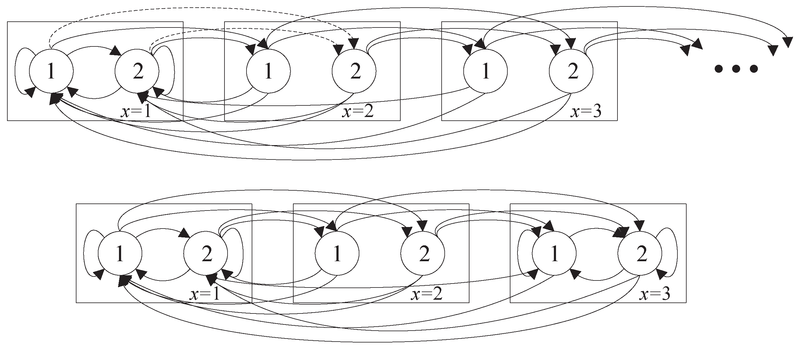
Finally, notice that the evolution of state $(x,q)$ forms a Markov chain as depicted in Figure 1 (top) for $Q=2$ as an example. We use ${\alpha }_{q,q^{\prime }}^x=\mathrm{Pr}\left((x+1,q^{\prime })\right|(x,q))$ and ${\beta }_{q,q^{\prime }}^x=\mathrm{Pr}\left((1,q^{\prime })\right|(x,q))$ to denote the transition probability between the states, which can be computed as follows,

$$\begin{array}{cc}\hfill {\alpha }_{q,q^{\prime }}^x& =\left\{\begin{array}{cc}(1-{\xi }_{x,q})p_{q{q}^{\prime }}+{\xi }_{x,q}{\epsilon }_q{p}_{q{q}^{\prime }},\hfill & x<X;\hfill \\ {\epsilon }_q{p}_{q{q}^{\prime }},\hfill & x\ge X.\hfill \end{array}\right.\hfill \end{array}$$

(14)

$$\begin{array}{cc}\hfill {\beta }_{q,q^{\prime }}^x& =\left\{\begin{array}{cc}{\xi }_{x,q}(1-{\epsilon }_q)p_{q{q}^{\prime }},\hfill & x<X;\hfill \\ (1-{\epsilon }_q)p_{q{q}^{\prime }},\hfill & x\ge X.\hfill \end{array}\right.\hfill \end{array}$$

(15)

According to the property of steady distribution, ${\mu }_{x,q}$ equals to the sum of the steady distribution which can be transferred to ${\mu }_{x,q}$ in the next slot times their transition probability. As depicted in Figure 1, ${\mu }_{2,2}={\mu }_{1,1}{\alpha }_{1,2}^1+{\mu }_{1,2}{\alpha }_{2,2}^1$ (see the dashed lines). Therefore, we can compute ${\mu }_{x,q}$ as follows,

$$\begin{array}{c}\hfill {\mu }_{x,q^{\prime }}=\left\{\begin{array}{cc}\sum _{q=1}^Q\sum _{x^{\prime }=1}^{\infty }{\beta }_{q,q^{\prime }}^{x^{\prime }}{\mu }_{x^{\prime },q},\hfill & x=1;\hfill \\ \sum _{q=1}^Q{\alpha }_{q,q^{\prime }}^{x-1}{\mu }_{x-1,q},\hfill & x\ge 2,\hfill \end{array}\right.\end{array}$$

which is equivalent to Equation (13c,d).    □

As the steady distribution is infinite, it is difficult to solve the problem exactly. Therefore, we approximate the optimization problem in Theorem 2 into a finite LP problem through truncation:

Problem 4

(Linear Programming Approximation).

$$\{{\tilde{\mu }}_{x,q}^{*},{\tilde{y}}_{x,q}^{*}\}=arg\underset{{\mu }_{x,q},y_{x,q}}{min}\sum _{q=1}^Q\sum _{x=1}^X(f\left(x\right){\mu }_{x,q}+\lambda y_{x,q}),$$

(16a)

$$\begin{array}{cc}\hfill s.t.& \sum _{q=1}^Q\sum _{x=1}^X{\mu }_{x,q}=1,\hfill \end{array}$$

(16b)

$$\begin{array}{cc}\hfill & {\mu }_{1,q^{\prime }}=\sum _{q=1}^Q\sum _{x=1}^X(1-{\epsilon }_q)p_{q{q}^{\prime }}{y}_{x,q},\hfill \end{array}$$

(16c)

$$\begin{array}{cc}\hfill & {\mu }_{x,q^{\prime }}=\sum _{q=1}^Q{p}_{q{q}^{\prime }}[{\mu }_{x-1,q}-(1-{\epsilon }_q)y_{x-1,q}],\forall 2\le x\le X-1,\hfill \end{array}$$

(16d)

$$\begin{array}{cc}\hfill & {\mu }_{X,q^{\prime }}=\sum _{q=1}^Q{p}_{q{q}^{\prime }}[{\mu }_{X-1,q}+{\mu }_{X,q}-(1-{\epsilon }_q)(y_{X-1,q}+y_{X,q})],\hfill \end{array}$$

(16e)

$$\begin{array}{cc}\hfill & \sum _{q=1}^Q\sum _{x=1}^X{y}_{x,q}w\left(q\right)\le \mathcal{E},\hfill \end{array}$$

(16f)

$$\begin{array}{cc}\hfill & 0\le {\mu }_{x,q}\le 1,0\le y_{x,q}\le {\mu }_{x,q},\hfill \end{array}$$

(16g)

$$\begin{array}{cc}\hfill & y_{X,q}={\mu }_{X,q}.\hfill \end{array}$$

(16h)

After truncation, the optimal value of Equation (16a) is the lower bound of the objective function of the decoupled problem Equation (8a). The detailed proof is provided in Appendix D. The key concept is to set a threshold X and convert the Markov chain into a finite-state one (see Figure 1).

Moreover, the following theorem guarantees the lower bound obtained by the above LP problem is tight when X is sufficiently large. Thus, the approximate optimal solution $\{{\tilde{\mu }}_{x,q}^{*},{\tilde{y}}_{x,q}^{*}\}$ performs close to the exact optimal solution $\{{\mu }_{x,q}^{*},y_{x,q}^{*}\}$. Before displaying the theorem, first denote ${\pi }_X^{*}$ and ${\pi }^{*}$ to be the scheduling policy according to the approximate optimal solution $\{{\tilde{\mu }}_{x,q}^{*},{\tilde{y}}_{x,q}^{*}\}$ by setting threshold X and optimal one $\{{\mu }_{x,q}^{*},y_{x,q}^{*}\}$, respectively. Define $J_{\infty }\left(\pi \right)$ to be the age and scheduling penalty of the primal problem under policy $\pi$ and $J_X\left(\pi \right)$ is the approximate penalty when we set the age penalty $f\left(x\right)=f\left(X\right),\forall x\ge X$. Then, according to Equations (13a) and (16a), we have

$$\begin{array}{c}\hfill J_{\infty }\left({\pi }^{*}\right)=\sum _{q=1}^Q\sum _{x=1}^{\infty }(f\left(x\right){\mu }_{x,q}^{*}+\lambda y_{x,q}^{*}),J_X\left({\pi }_X^{*}\right)=\sum _{q=1}^Q\sum _{x=1}^X(f\left(x\right){\tilde{\mu }}_{x,q}^{*}+\lambda {\tilde{y}}_{x,q}^{*}).\end{array}$$

Theorem 3.

Assume $f\left(x\right)$ satisfies the following property: $\exists ϵ\in [\sqrt{{\epsilon }_{\max }},1)$ and constant $k>0$ such that $f\left(X\right)=k{ϵ}^{-X}$ and $f\left(x\right)\le k{ϵ}^{-x},\forall x\ge X$, where ${\epsilon }_{\max }={max}_q{\epsilon }_q$. Then, we have the following property,

$$J_{\infty }\left({\pi }^{*}\right)-J_X\left({\pi }_X^{*}\right)\le \frac{k{\epsilon }_{\max }^{\frac{X+1}{2}-{\tau }_{\max }}}{1-{\epsilon }_{\max }},$$

(17)

where ${\tau }_{\max }={max}_q{\tau }_q$. As we see the above inequality, the difference between optimal solution of Theorem 2 and Problem 4 converges to 0 as the threshold X becomes sufficiently large.

The entire proof is provided in Appendix E.

After solving the above LP problem, we can obtain the approximate optimal scheduling probability $\left\{{\tilde{\xi }}_{x,q}^{*}\right\}$ by setting a sufficiently large X and computing $\left\{{\tilde{\mu }}_{x,q}^{*}\right\}$ and $\left\{{\tilde{y}}_{x,q}^{*}\right\}$. Moreover, analogical to the threshold structure described in Lemma 1, $\left\{{\tilde{\xi }}_{x,q}^{*}\right\}$ also has the following property.

Lemma 2.

For any state $(x,q)$ of each sensor, the optimal scheduling probability $\left\{{\tilde{\xi }}_{x,q}^{*}\right\}$ is non-decreasing with x, i.e.,

$${\tilde{\xi }}_{x_1,q}^{*}\le {\tilde{\xi }}_{x_2,q}^{*},\forall x_1\le x_2.$$

The proof technique is similar to Lemma 1, so it is omitted here.

5. Multi-Sensor Problem Resolution

By now, through relaxing, decoupling and truncation, we have obtained the approximate solution to the single-sensor decoupled problem for fixed scheduling penalty $\lambda$. In this section, we will go back to solve the multi-sensor problem, and propose a truncated policy to meet the hard bandwidth constraint in Equation (6b).

5.1. The Relaxed Problem Resolution

First, we should choose the optimal $\lambda$ such that the relaxed bandwidth constraint can be fully leveraged. Denote $g\left(\lambda \right)={min}_{\pi }L(\pi ,\lambda )$ to be the Lagrange dual function, where we choose the approximate optimal policy ${\pi }^{*}\left(\lambda \right)$ by solving LP. Then, the dual function can be computed as follows,

$$g\left(\lambda \right)=\frac{1}{N}\left(\sum _{n=1}^N{g}_n\left(\lambda \right)-\lambda M\right),$$

where $g_n\left(\lambda \right)={min}_{\pi }{L}_n(\pi ,\lambda )$ is the decoupled dual function for sensor n. According to the LP approximation, $g_n\left(\lambda \right)$ can be further written out as follows,

$$\begin{array}{c}\hfill g_n\left(\lambda \right)=X_n\left(\lambda \right)+\lambda U_n\left(\lambda \right),\end{array}$$

where $X_n\left(\lambda \right)$ is the average age penalty bounded by ${\sum }_{x=1}^X{\sum }_{q=1}^{Q}f\left(x\right){\tilde{\mu }}_{x,q}^{n,*}$, and $U_n\left(\lambda \right)$ is the average scheduling probability, which equals to ${\sum }_{x=1}^X{\tilde{y}}_{x,q}^{n,*}$.

According to the work in [24], the optimal Lagrange multiplier ${\lambda }^{*}$ satisfies

$$\begin{array}{c}\hfill {\lambda }^{*}=sup\left\{\lambda \right|\sum _{n=1}^N{U}_n\left(\lambda \right)\le M\}.\end{array}$$

If $U_n\left({\lambda }^{*}\right)=M$, then the optimal policy is just $\pi \left({\lambda }^{*}\right)$. Otherwise, the optimal policy is a mixture of two policies, denoted by ${\pi }_l$ and ${\pi }_u$, which can be computed by

$$\begin{array}{c}\hfill {\pi }_l=\underset{\lambda \to {\lambda }^{*-}}{lim}\pi \left(\lambda \right),{\pi }_u=\underset{\lambda \to {\lambda }^{*+}}{lim}\pi \left(\lambda \right).\end{array}$$

Then, we apply the sub-gradient ascend method to find the optimal solution, where the sub-gradient can be computed as follows,

$${\mathrm{d}}_{\lambda }g\left(\lambda \right)=\sum _{n=1}^N{U}_n\left(\lambda \right)-M=U\left(\lambda \right)-M,$$

(18)

where $U\left(\lambda \right)={\sum }_{n=1}^N{U}_n\left(\lambda \right)$ is the total scheduling probability.

Choose ${\lambda }_0=0$ as the starting point, and compute the average scheduling probability $U\left({\lambda }_0\right)$. If $U\left({\lambda }_0\right)<M$, then it does not need to consider the bandwidth constraint, and thus the optimal solution has already been solved. Moreover, this optimal solution can also be viewed as the lower bound of the primal optimization problem, i.e.,

$$\mathrm{LB}=\frac{1}{N}\sum _{n=1}^N\sum _{x=1}^X\sum _{q=1}^{Q}f\left(x\right){\tilde{\mu }}_{x,q}^{n,*}\left({\lambda }_0\right).$$

Otherwise, we need to increase the scheduling penalty through iterations. The update operation in iteration k can be written out as follows,

$${\lambda }_{k+1}={\lambda }_k+t_{k+1}{\mathrm{d}}_{\lambda }g\left({\lambda }_k\right),$$

where $t_{k+1}$ is the step size in iteration k.

Moreover, the step size is determined as follows,

$$\begin{array}{c}\hfill t_{k+1}=\left\{\begin{array}{cc}\gamma t_k,\hfill & {\mathrm{d}}_{\lambda }g\left({\lambda }_k\right){\mathrm{d}}_{\lambda }g\left({\lambda }_{k-1}\right)<0;\hfill \\ t_k,\hfill & \mathrm{otherwise},\hfill \end{array}\right.\end{array}$$

where $\gamma \in (0,1)$ is a constant.

The determination of the step size above guarantees the algorithm converges from both sides. Therefore, after running the whole algorithm, we can obtain two different scheduling probabilities $M_l$ and $M_u$:

$$\begin{array}{cc}\hfill M_l& =\underset{k}{max}U\left({\lambda }_k\right),\mathrm{s}.\mathrm{t}.{\mathrm{d}}_{\lambda }g\left({\lambda }_k\right)\le 0;\hfill \end{array}$$

(19)

$$\begin{array}{cc}\hfill M_u& =\underset{k}{min}U\left({\lambda }_k\right),\mathrm{s}.\mathrm{t}.{\mathrm{d}}_{\lambda }g\left({\lambda }_k\right)\ge 0.\hfill \end{array}$$

(20)

Their corresponding optimal polices are denoted as $\{{\tilde{\mu }}_{x,q}^{n,l},{\tilde{y}}_{x,q}^{n,l}\}$ and $\{{\tilde{\mu }}_{x,q}^{n,u},{\tilde{y}}_{x,q}^{n,u}\}$. Then, the optimal stationary policy can be obtained by mixing these two policies:

$$\{{\tilde{\mu }}_{x,q}^{n,*},{\tilde{y}}_{x,q}^{n,*}\}=\theta \{{\tilde{\mu }}_{x,q}^{n,u},{\tilde{y}}_{x,q}^{n,u}\}+(1-\theta )\{{\tilde{\mu }}_{x,q}^{n,l},{\tilde{y}}_{x,q}^{n,l}\},$$

where the mixed coefficient can be computed as follows,

$$\theta =\frac{M-M_l}{M_u-M_l}.$$

Now, we have obtained the optimal stationary policy of the relaxed scheduling problem. The algorithm flow chart is listed in Algorithm 1. Once we obtain $\{{\tilde{\mu }}_{x,q}^{n,*},{\tilde{y}}_{x,q}^{n,*}\}$, the optimal scheduling probability $\left\{{\tilde{\xi }}_{x,q}^{n,*}\right\}$ can be computed as follows,

$$\begin{array}{c}\hfill {\tilde{\xi }}_{x,q}^{n,*}=\left\{\begin{array}{cc}1,\hfill & \mathrm{if}x>X\mathrm{or}{\tilde{\mu }}_{x,q}^{n,*}=0\mathrm{or}{\tilde{\xi }}_{x-1,q}^{n,*}=1;\hfill \\ \frac{{\tilde{y}}_{x,q}^{n,*}}{{\tilde{\mu }}_{x,q}^{n,*}},\hfill & \mathrm{otherwise}.\hfill \end{array}\right.\end{array}$$

Algorithm 1 Construction of the optimal stationary policy

Initialization: ${\lambda }_{-1}={\lambda }_0=0$, $ϵ$, $t_0$, $\gamma$, $M_u$ and $M_l$

for each $n\in [1,N]$ do

compute $\{{\tilde{\mu }}_{x,q}^{n,*}\left({\lambda }_0\right),{\tilde{y}}_{x,q}^{n,*}\left({\lambda }_0\right)\}$ and $U_n\left({\lambda }_0\right)$

end for

if ${\mathrm{d}}_{\lambda }g\left({\lambda }_0\right)\le 0$ then

$\{{\tilde{\mu }}_{x,q}^{n,*},{\tilde{y}}_{x,q}^{n,*}\}=\{{\tilde{\mu }}_{x,q}^{n,*}\left({\lambda }_0\right),{\tilde{y}}_{x,q}^{n,*}\left({\lambda }_0\right)\}$

else

$k=0$

while $|{\lambda }_k-{\lambda }_{k-1}|>ϵ$ or ${\mathrm{d}}_{\lambda }g\left({\lambda }_k\right)>0$ do

if ${\mathrm{d}}_{\lambda }g\left({\lambda }_k\right){\mathrm{d}}_{\lambda }g\left({\lambda }_{k-1}\right)<0$ then

$t_{k+1}=\gamma t_k$

else

$t_{k+1}=t_k$

end if

${\lambda }_{k+1}={\lambda }_k+t_{k+1}{\mathrm{d}}_{\lambda }g\left({\lambda }_k\right)$

for each $n\in [1,N]$ do

compute $\{{\tilde{\mu }}_{x,q}^{n,*}\left({\lambda }_{k+1}\right),{\tilde{y}}_{x,q}^{n,*}\left({\lambda }_{k+1}\right)\}$ and $U_n\left({\lambda }_{k+1}\right)$

end for

if ${\mathrm{d}}_{\lambda }g\left({\lambda }_{k+1}\right)\ge 0$ and $U\left({\lambda }_{k+1}\right)\le M_u$ then

$\{{\tilde{\mu }}_{x,q}^{n,u},{\tilde{y}}_{x,q}^{n,u}\}=\{{\tilde{\mu }}_{x,q}^{n,*}\left({\lambda }_{k+1}\right),{\tilde{y}}_{x,q}^{n,*}\left({\lambda }_{k+1}\right)\}$

$M_u=U\left({\lambda }_{k+1}\right)$

end if

if ${\mathrm{d}}_{\lambda }g\left({\lambda }_{k+1}\right)\le 0$ and $U\left({\lambda }_{k+1}\right)\ge M_l$ then

$\{{\tilde{\mu }}_{x,q}^{n,l},{\tilde{y}}_{x,q}^{n,l}\}=\{{\tilde{\mu }}_{x,q}^{n,*}\left({\lambda }_{k+1}\right),{\tilde{y}}_{x,q}^{n,*}\left({\lambda }_{k+1}\right)\}$

$M_l=U\left({\lambda }_{k+1}\right)$

end if

$k=k+1$

end while

$\theta =\frac{M-M_l}{M_u-M_l}$

$\{{\tilde{\mu }}_{x,q}^{n,*},{\tilde{y}}_{x,q}^{n,*}\}=\theta \{{\tilde{\mu }}_{x,q}^{n,u},{\tilde{y}}_{x,q}^{n,u}\}+(1-\theta )\{{\tilde{\mu }}_{x,q}^{n,l},{\tilde{y}}_{x,q}^{n,l}\}$

end if

5.2. Truncation for the Hard Bandwidth Constraint

Finally, a bandwidth-truncated policy ${\widehat{\pi }}_X$ is derived from the optimal stationary policy ${\pi }_X^{*}$ to satisfy the hard bandwidth constraint in Equation (6b). Before introducing the truncated policy, first denote $S\left(t\right)$ to be the set of sensors to be scheduled in slot t, and $\left|S\right(t\left)\right|$ is the number of sensors to be scheduled in slot t. Then, the construction of ${\widehat{\pi }}_X$ is carried out as follows.

• In slot t, compute the scheduling set $S\left(t\right)$ according to the optimal stationary policy ${\pi }_X^{*}$.
• If $\left|S\right(t\left)\right|\le M$, then ${\widehat{\pi }}_X$ schedules all these sensors as ${\pi }_X^{*}$ does.
• If $\left|S\right(t\left)\right|>M$, the hard bandwidth constraint is never satisfied. Therefore, ${\widehat{\pi }}_X$ randomly chooses M out of $\left|S\right(t\left)\right|$ sensors to be scheduled in the current slot.

The following theorem guarantees the asymptotic performance of the truncated policy ${\widehat{\pi }}_X$ compared with ${\pi }_X^{*}$ on certain conditions.

Theorem 4.

Suppose the age penalty function is concave, and let $\kappa =\frac{M}{N}$ be a constant. If all the sensors and their channels are identical, i.e., the power constraint and the channel transition matrix are the same, then the truncated policy ${\widehat{\pi }}_X$ and the optimal randomized policy ${\pi }_X^{*}$ have the following property,

$$\underset{N\to \infty }{lim}J\left({\widehat{\pi }}_X\right)-J\left({\pi }_X^{*}\right)=0.$$

The whole proof is provided in Appendix F.

6. Simulation Results

In this section, we provide simulation results to verify the performance of the proposed policy. First, we study the average age penalty performance with different types of sensors with different bandwidth constraint and AoI truncation threshold X. Next, we study the detailed scheduling decision of each sensor. The average performance is obtained by simulating ${10}^5$ consecutive slots.

6.1. Average Age Penalty Performance

In this part, we demonstrate the average performance of our proposed policy. We consider 4-state channel system, i.e., $Q=4$. The age penalty function is chosen as $f\left(x\right)=ln\left(x\right)$ unless otherwise specified. The transition matrix ${\mathit{P}}_n$ for each sensor is the same:

$${\mathit{P}}_n=\left(\begin{array}{cccc}0.4& 0.3& 0.2& 0.1\\ 0.25& 0.3& 0.25& 0.2\\ 0.2& 0.25& 0.3& 0.25\\ 0.1& 0.2& 0.3& 0.4\end{array}\right).$$

(21)

Denote $\left\{{\eta }_q\right\}$ to be the steady distribution of the channel state. We consider that for each channel state q, the energy consumption $w\left(q\right)=q$. According to [12], the optimal policy to minimize the average AoI performance when all the sensors are identical is a greedy policy, which schedules the M sensors with the largest AoI and consumes the average power for each sensor ${\mathcal{E}}_G=\frac{M}{N}{\sum }_{q=1}^Q{\eta }_{q}w\left(q\right)$. Therefore, define ${\rho }_n=\frac{{\mathcal{E}}_n}{{\mathcal{E}}_G}$ to be the power constraint factor which describes the effects of power consumption constraint ${\mathcal{E}}_n$.

Figure 2 demonstrates the average age penalty performance of the proposed policy ${\widehat{\pi }}_X$ as a number of sensors N, with bandwidth constraint $M=\{5,15\}$, compared with the lower bound, the relaxed optimal policy ${\pi }_X^{*}$ and the greedy policy. Set the threshold $X=\lceil \frac{20N}{M}\rceil$, where $\lceil ·\rceil$ is ceiling function. We assume that the probability of packet loss for each sensor is the same, denoted by $\epsilon$:

$$\epsilon =[0.1,0.3,0.2,0.4].$$

The power constraint factor of sensor n is ${\rho }_n=0.2+\frac{1.4(n-1)}{N-1}$.

As seen in Figure 2, the proposed truncated policy performs closely to the relaxed optimal policy and the lower bound, and outperforms the greedy policy especially when N is large. According to Figure 2, the age penalty decreases by $18\%$ and $23\%$ from the greedy policy with $N=60$ sensors when $M=5$ and $M=15$, respectively, under proposed policy. Moreover, as the threshold X becomes large, the difference between the average performance following policy ${\pi }_X^{*}$ and the lower bound becomes indistinguishable. Therefore, the asymptotic performance described in Theorem 3 can be verified.

Figure 3 compares the average performance of the proposed policy ${\widehat{\pi }}_X$ with the AoI-minimum policy to verify the improvement of considering different penalty function. The AoI-minimum policy is similar to the one proposed in our previous work [22] with the consideration of packet loss. The bandwidth constraint $M=2$. The packet loss probability $\epsilon =[0.25,0.35,0.65,0.8]$, and the energy consumption $w\left(q\right)=2^q$. Here the age penalty function is chosen as $f\left(x\right)=x^2$. From Figure 3, we can see that the AoI-minimum policy cannot guarantee a good age penalty performance. Thus, it is necessary to consider different demand for data freshness to achieve better performance.

Figure 4 and Figure 5 verify the asymptotic performance of the proposed policy with different age penalty function and different packet loss probability respectively when $M/N$ is a constant in symmetric networks. From both figures, it can be seen that the difference of average age penalty under proposed policy and the lower bound becomes small as N increases. Thus, the asymptotic performance described in Theorem 4 can be verified.

6.2. Sensor Level Analysis and Threshold Structure

Next, we analyze the scheduling decision of each sensor and their corresponding age penalty to provide some insights of optimal scheduling policies. We consider a system with $N=8$ and $M=2$. The transition matrix of channel state is the same as Equation (21), and power consumption $w\left(q\right)=q$. We set the threshold $X=80$ to compute the proposed policy.

First we consider the system with $Q=4$ and age penalty function $f\left(x\right)=lnx$. Figure 6 analyzes how the power constraint influences age penalty of each sensor. The power constraint of sensor n is ${\rho }_n=0.2n$. From Figure 6, we can see that the proposed policy outperforms the greedy policy when the required power consumption is scarce, and performs similarly or a little worse when the factor ${\rho }_n>1$. This implies that our proposed policy chooses a more proper power allocation based on current channel state and AoI than the greedy policy by stimulating sources with scarce power budgets to be scheduled in better channel states.

As the packet loss influences age penalty as well, Figure 7 considers sensors with different probability of packet loss, which can be written out as the following matrix $\left\{{\epsilon }_{n,q}\right\}$:

$$\epsilon =\left(\begin{array}{cccc}0.05& 0.1& 0.15& 0.2\\ 0.1& 0.15& 0.2& 0.25\\ 0.15& 0.2& 0.25& 0.3\\ 0.2& 0.25& 0.3& 0.35\\ 0.25& 0.3& 0.35& 0.4\\ 0.3& 0.35& 0.4& 0.45\\ 0.35& 0.4& 0.45& 0.5\\ 0.4& 0.45& 0.5& 0.55\end{array}\right).$$

(22)

We fix the power constraint factor ${\rho }_n=0.6$ for all sensors. Figure 7 shows that the average age penalty increases with the probability of packet loss. Moreover, the proposed policy combats with the packet loss better than the greedy policy as the proposed policy considers ${\epsilon }_{n,q}$ when solving the LP problem, but the greedy policy does not.

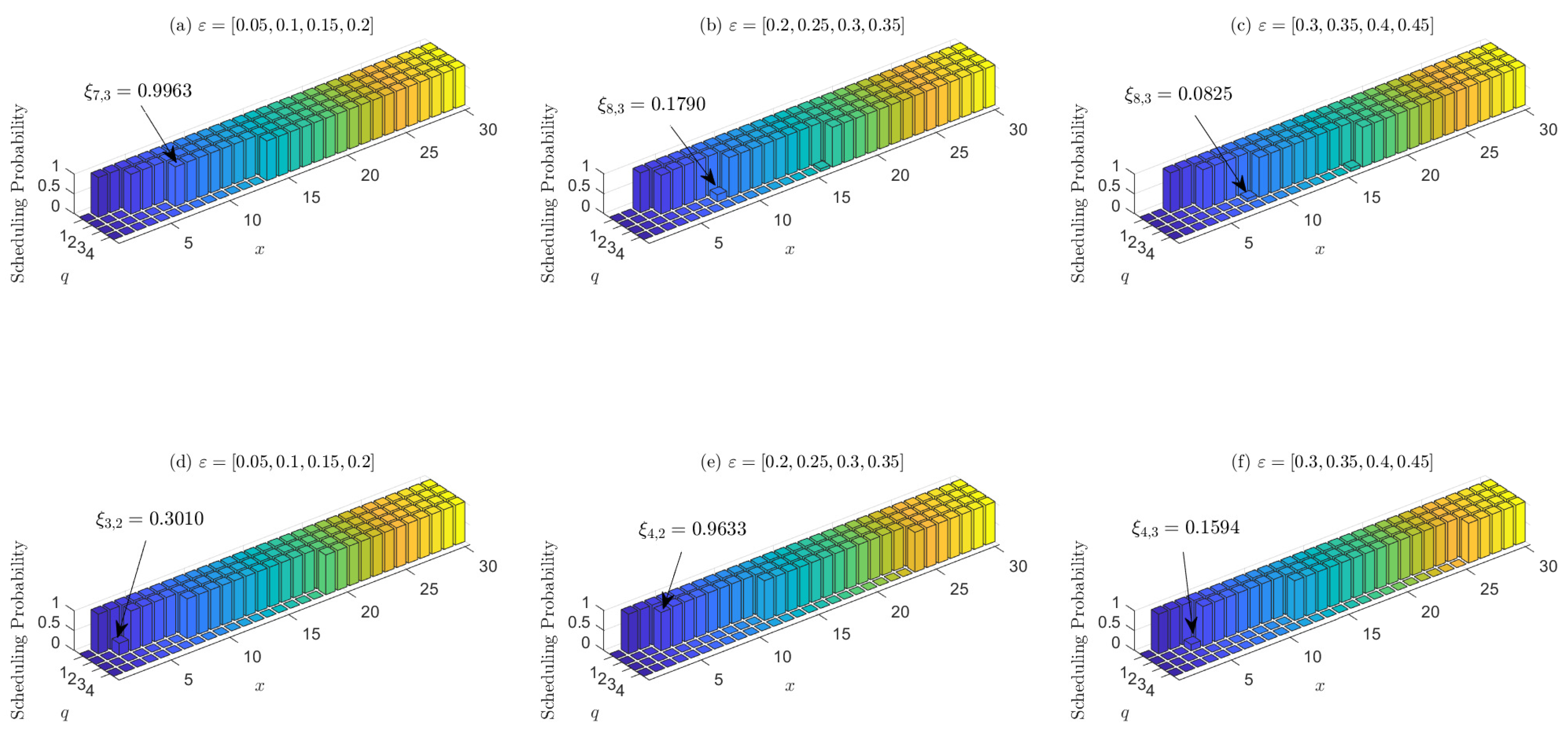
Next, we verify the threshold structure of the optimal scheduling policy. Figure 8 demonstrates the effect of bandwidth and packet loss on the scheduling threshold. The power constraint factor ${\rho }_n=0.6,\forall n$, and the packet loss probability is the same as Equation (22). Subfigures (a–c) demonstrate three of these sensors whose packet loss probability is as the title. For each of the three sensors, subfigures (d–f) consider the single-sensor system without bandwidth constraint and display their scheduling probability, respectively. Moreover, Figure 8 lists some of the thresholds given channel state q, e.g., in subfigure (a), the threshold of channel state $q=3$ is $x=7$, and the corresponding optimal scheduling probability is ${\xi }_{7,3}=0.9963$. From Figure 8, first we can see that all the six figures verify the non-decreasing property of the scheduling probability with AoI $x\left(t\right)$ described in Lemma 2. Second, subfigures (a–c) demonstrate that the sensor with higher packet loss probability also has higher scheduling threshold. This implies that the sensors with more reliable channel should be given higher priority to scheduling than unreliable ones to minimize the average age penalty, since scheduling the more reliable channel under the same AoI is more likely to reduce the current age penalty. Third, by comparing subfigures (a) and (d), (b) and (e), and (c) and (f), the scheduling threshold varies more significantly for different channel states if there exists no bandwidth constraint. The sensors tend to update more often when the channel state is good, and idle when the channel state is bad. This is because the sensors can choose to update packets more frequently in good channel state to both save energy and increase the success probability of transmission without bandwidth constraint.

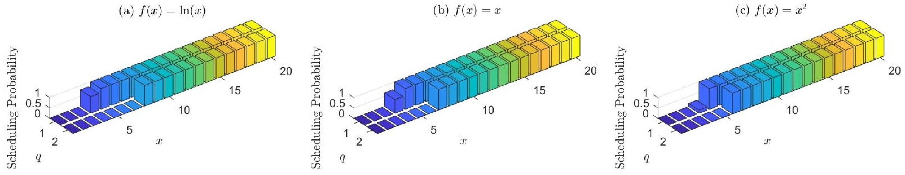
Finally, we study the effects of age penalty function on threshold structure. Here, we consider a system with $Q=2$, ${\rho }_n=0.2n$ and three different penalty function, i.e., $f\left(x\right)=lnx$, $f\left(x\right)=x$, and $f\left(x\right)=x^2$ in Figure 9. We plot the scheduling decision of the sixth sensor. As is depicted in Figure 9, as the system has a higher restriction on data freshness such as exponential or quadratic function, the difference between thresholds of different states becomes small. In such situations, channel states play a weaker role because waiting for another slot to schedule tends to have unbearable age penalty.

7. Conclusions

In this paper, we consider the multi-sensor scheduling problem through an error-prone Markovian channel state. Through relaxing and decoupling, we propose a truncated policy to satisfy both the bandwidth and power constraints to minimize the average age penalty of all sensors in infinite horizon. We prove the asymptotic performance of the truncated policy in symmetric networks when the age penalty function is concave by choosing a sufficiently large threshold X. Through theoretical analysis and numerical simulations, we find that the age penalty function, packet loss probability, bandwidth constraint, and power constraint work altogether to influence the optimal scheduling decisions. Those who have more reliable channel state and enough power consumption tend to have higher scheduling priority.

References

- Kaul, S.; Gruteser, M.; Rai, V.; Kenney, J. Minimizing age of information in vehicular networks. In Proceedings of the 2011 8th Annual IEEE Communications Society Conference on Sensor, Mesh and Ad Hoc Communications and Networks, Salt Lake City, UT, USA, 27–30 June 2011; pp. 350–358. [Google Scholar]
- Zhou, B.; Saad, W. Optimal Sampling and Updating for Minimizing Age of Information in the Internet of Things. In Proceedings of the 2018 IEEE Global Communications Conference (GLOBECOM), Abu Dhabi, UAE, 9–13 December 2018; pp. 1–6. [Google Scholar]
- Kaul, S.; Yates, R.; Gruteser, M. Real-time status: How often should one update? In Proceedings of the 2012 Proceedings IEEE INFOCOM, Orlando, FL, USA, 25–30 March 2012; pp. 2731–2735. [Google Scholar]
- Chen, K.; Huang, L. Age-of-information in the presence of error. In Proceedings of the 2016 IEEE International Symposium on Information Theory (ISIT), Barcelona, Spain, 10–15 July 2016; pp. 2579–2583. [Google Scholar]
- Costa, M.; Codreanu, M.; Ephremides, A. On the Age of Information in Status Update Systems with Packet Management. IEEE Trans. Inf. Theory 2016, 62, 1897–1910. [Google Scholar] [CrossRef]
- Najm, E.; Yates, R.; Soljanin, E. Status updates through M/G/1/1 queues with HARQ. In Proceedings of the 2017 IEEE International Symposium on Information Theory (ISIT), Aachen, Germany, 25–30 June 2017; pp. 131–135. [Google Scholar]
- Kosta, A.; Pappas, N.; Ephremides, A.; Angelakis, V. Age and value of information: Non-linear age case. In Proceedings of the 2017 IEEE International Symposium on Information Theory (ISIT), Aachen, Germany, 25–30 June 2017; pp. 326–330. [Google Scholar]
- Wang, X.; Duan, L. Dynamic Pricing for Controlling Age of Information. In Proceedings of the 2019 IEEE International Symposium on Information Theory (ISIT), Paris, France, 7–12 July 2019; pp. 962–966. [Google Scholar]
- Sun, Y.; Uysal-Biyikoglu, E.; Yates, R.; Koksal, C.E.; Shroff, N.B. Update or wait: How to keep your data fresh. IEEE Trans. Inf. Theory 2017, 63, 7492–7508. [Google Scholar] [CrossRef]
- Ceran, E.T.; Gündüz, D.; György, A. Average Age of Information With Hybrid ARQ Under a Resource Constraint. IEEE Trans. Wirel. Commun. 2019, 18, 1900–1913. [Google Scholar] [CrossRef] [Green Version]
- Bacinoglu, B.T.; Ceran, E.T.; Uysal-Biyikoglu, E. Age of information under energy replenishment constraints. In Proceedings of the 2015 Information Theory and Applications Workshop (ITA), San Diego, CA, USA, 1–6 February 2015; pp. 25–31. [Google Scholar]
- Kadota, I.; Uysal-Biyikoglu, E.; Singh, R.; Modiano, E. Minimizing the Age of Information in broadcast wireless networks. In Proceedings of the 2016 54th Annual Allerton Conference on Communication, Control, and Computing (Allerton), Monticello, IL, USA, 27–30 September 2016; pp. 844–851. [Google Scholar]
- Maatouk, A.; Kriouile, S.; Assaad, M.; Ephremides, A. On the Optimality of the Whittle’s Index Policy for Minimizing the Age of Information. arXiv 2020, arXiv:2001.03096. [Google Scholar] [CrossRef]
- Kadota, I.; Sinha, A.; Modiano, E. Scheduling Algorithms for Optimizing Age of Information in Wireless Networks with Throughput Constraints. IEEE/ACM Trans. Netw. 2019, 27, 1359–1372. [Google Scholar] [CrossRef]
- Kadota, I.; Sinha, A.; Uysal-Biyikoglu, E.; Singh, R.; Modiano, E. Scheduling Policies for Minimizing Age of Information in Broadcast Wireless Networks. IEEE/ACM Trans. Netw. 2018, 26, 2637–2650. [Google Scholar] [CrossRef] [Green Version]
- Bedewy, A.M.; Sun, Y.; Shroff, N.B. Age-optimal information updates in multihop networks. In Proceedings of the 2017 IEEE International Symposium on Information Theory (ISIT), Aachen, Germany, 25–30 June 2017; pp. 576–580. [Google Scholar]
- Chen, X.; Gatsis, K.; Hassani, H.; Bidokhti, S.S. Age of Information in Random Access Channels. In Proceedings of the 2020 IEEE International Symposium on Information Theory (ISIT), Los Angeles, CA, USA, 21–26 June 2020. [Google Scholar]
- Hsu, Y.; Modiano, E.; Duan, L. Age of information: Design and analysis of optimal scheduling algorithms. In Proceedings of the 2017 IEEE International Symposium on Information Theory (ISIT), Aachen, Germany, 25–30 June 2017; pp. 561–565. [Google Scholar]
- Talak, R.; Kadota, I.; Karaman, S.; Modiano, E. Scheduling Policies for Age Minimization in Wireless Networks with Unknown Channel State. In Proceedings of the 2018 IEEE International Symposium on Information Theory (ISIT), Vail, CO, USA, 17–22 June 2018; pp. 2564–2568. [Google Scholar]
- Sun, Y.; Polyanskiy, Y.; Uysal, E. Sampling of the Wiener Process for Remote Estimation over a Channel with Random Delay. IEEE Trans. Inf. Theory 2019, 66, 1118–1135. [Google Scholar] [CrossRef]
- Wang, J.; Ren, X.; Mo, Y.; Shi, L. Whittle Index Policy for Dynamic Multichannel Allocation in Remote State Estimation. IEEE Trans. Autom. Control 2020, 65, 591–603. [Google Scholar] [CrossRef]
- Tang, H.; Wang, J.; Song, L.; Song, J. Minimizing Age of Information With Power Constraints: Multi-User Opportunistic Scheduling in Multi-State Time-Varying Channels. IEEE J. Sel. Areas Commun. 2020, 38, 854–868. [Google Scholar] [CrossRef] [Green Version]
- Wu, S.; Han, D.; Cheng, P.; Shi, L. Optimal Scheduling of Multiple Sensors over Lossy and Bandwidth Limited Channels. arXiv 2018, arXiv:1804.05618. [Google Scholar] [CrossRef] [Green Version]
- Beutler, F.J.; Ross, K.W. Optimal policies for controlled Markov chains with a constraint. J. Math. Anal. Appl. 1985, 112, 236–252. [Google Scholar] [CrossRef] [Green Version]
- Tajan, R.; Ciblat, P. Information-theoretic multi-user power adaptation in retransmission schemes. In Proceedings of the 2016 IEEE 17th International Workshop on Signal Processing Advances in Wireless Communications (SPAWC), Edinburgh, UK, 3–6 July 2016; pp. 1–5. [Google Scholar]
- Hernández-Lerma, O.; Lasserre, J.B. Discrete-Time Markov Control Processes: Basic Optimality Criteria; Springer Science & Business Media: Berlin, Germany, 2012; Volume 30. [Google Scholar]
- Diaconis, P.; Zabell, S. Closed form summation for classical distributions: Variations on a theme of de Moivre. Stat. Sci. 1991, 6, 284–302. [Google Scholar] [CrossRef]
Figure 1.
Illustration of the state transition graph for channel states without (top) and with (bottom) AoI truncation with AoI threshold . The numbers in circles are channel state index q, and the number in rectangles are AoI index x.
Figure 2.
Average age penalty performance as a number of sensors N, .
Figure 3.
Average age penalty performance as a number of sensors N compared with AoI-minimum policy.
Figure 4.
Asymptotic average age penalty performance with different age penalty function . .
Figure 5.
Asymptotic average age penalty performance with different packet loss probability.
. .
Figure 6.
Each sensor’s average penalty with different power constraint factor .
Figure 7.
Each sensor’s average penalty with different packet loss probability .
Figure 8.
Subfigures (a–c) demonstrate the scheduling probability of sensors whose packet loss probability is as the title when and . Subfigures (d–f) demonstrate their scheduling probability in single-sensor system respectively. All the power constraint is .
Figure 9.
Threshold comparison with different age penalty function.
Publisher’s Note: MDPI stays neutral with regard to jurisdictional claims in published maps and institutional affiliations. |
© 2021 by the authors. Licensee MDPI, Basel, Switzerland. This article is an open access article distributed under the terms and conditions of the Creative Commons Attribution (CC BY) license (http://creativecommons.org/licenses/by/4.0/).
Share and Cite
MDPI and ACS Style
Chen, Y.; Tang, H.; Wang, J.; Song, J. Optimizing Age Penalty in Time-Varying Networks with Markovian and Error-Prone Channel State. Entropy 2021, 23, 91. https://0-doi-org.brum.beds.ac.uk/10.3390/e23010091
AMA Style
Chen Y, Tang H, Wang J, Song J. Optimizing Age Penalty in Time-Varying Networks with Markovian and Error-Prone Channel State. Entropy. 2021; 23(1):91. https://0-doi-org.brum.beds.ac.uk/10.3390/e23010091
Chicago/Turabian StyleChen, Yuchao, Haoyue Tang, Jintao Wang, and Jian Song. 2021. "Optimizing Age Penalty in Time-Varying Networks with Markovian and Error-Prone Channel State" Entropy 23, no. 1: 91. https://0-doi-org.brum.beds.ac.uk/10.3390/e23010091
Note that from the first issue of 2016, this journal uses article numbers instead of page numbers. See further details here.