
Information Geometry, Fluctuations, Non-Equilibrium Thermodynamics, and Geodesics in Complex Systems


Center for Fluid and Complex Systems, Coventry University, Priory St, Coventry CV1 5FB, UK
Entropy 2021, 23(11), 1393; https://0-doi-org.brum.beds.ac.uk/10.3390/e23111393
Submission received: 29 September 2021
/
Revised: 15 October 2021
/
Accepted: 19 October 2021
/
Published: 24 October 2021
(This article belongs to the Special Issue Review Papers for Entropy)
Abstract
:Information theory provides an interdisciplinary method to understand important phenomena in many research fields ranging from astrophysical and laboratory fluids/plasmas to biological systems. In particular, information geometric theory enables us to envision the evolution of non-equilibrium processes in terms of a (dimensionless) distance by quantifying how information unfolds over time as a probability density function (PDF) evolves in time. Here, we discuss some recent developments in information geometric theory focusing on time-dependent dynamic aspects of non-equilibrium processes (e.g., time-varying mean value, time-varying variance, or temperature, etc.) and their thermodynamic and physical/biological implications. We compare different distances between two given PDFs and highlight the importance of a path-dependent distance for a time-dependent PDF. We then discuss the role of the information rate and relative entropy in non-equilibrium thermodynamic relations (entropy production rate, heat flux, dissipated work, non-equilibrium free energy, etc.), and various inequalities among them. Here, is the information length representing the total number of statistically distinguishable states a PDF evolves through over time. We explore the implications of a geodesic solution in information geometry for self-organization and control.
1. Introduction
Information geometry refers to the application of the techniques of differential geometry to probability and statistics. Specifically, it uses differential geometry to define the metric tensor that endows the statistical space (consisting of probabilities) with the notion of distance [1,2,3,4,5,6,7,8,9,10,11,12,13,14,15,16,17,18,19,20,21,22,23,24,25,26,27,28,29,30,31]. While seemingly too abstract, it permits us to measure quantitative differences among different probabilities. It then makes it possible to link a stochastic process, complexity, and geometry, which is particularly useful in classifying a growing number of data from different research areas (e.g., from astrophysical and laboratory systems to biosystems). Furthermore, it can be used to obtain desired outcomes [6,7,8,9,10,15] or to understand statistical complexity [4].
For instance, the Wasserstein metric [6,7,8,9,10] was widely used in the optimal transport problem where the main interest is to minimize transport cost which is a quadratic function of the distance between two locations. It satisfies the Fokker-Planck equation for gradient flow which minimizes the entropy/energy functional [7]. For Gaussian distributions, the Wasserstein metric space consists of physical distances – Euclidean and positive symmetric matrices for the mean and variance, respectively (e.g., see [8]).
In comparsion, the Fisher (Fisher-Rao) information [32] can be used to define a dimensionless distance in statistical manifolds [33,34]. For instance, the statistical distance represents the number of indistinguishable states as [5,33]
Here the Fisher information metric provides natural (Riemannian) distinguishability metric on the space of probability distributions. ’s are the parameters of the probability and the angular brackets represent the ensemble average over . Note that Equation (1) is given for a discrete probability . For a continuous Probability Density Function (PDF) for a variable x, Equation (1) becomes where .
For Gaussian processes, the Fisher metric is inversely proportional to the covariance matrices of fluctuations in the systems. Thus, in thermodynamic equilibrium, strong fluctuations lead to a strong correlation and a shorter distance between the neighboring states [34,35]. Alternatively, fluctuations determine the uncertainty in measurements, providing the resolution (the distance unit) that normalizes the distance between different thermodynamic states.
To appreciate the meaning of fluctuation-based metric, let us consider the (equilibrium) Maxwell-Boltzmann distribution for the energy state
Here is the inverse temperature; is the Boltzmann constant; T is the temperature of the heat bath. In Equation (2), the thermal energy of the heat bath (the width/uncertainty of the probability) provides the resolution to differentiate different states . The smaller is the resolution (temperature), the more distinguishable states (more accessible information in the system) there are. It agrees with the expectation that a PDF gradient (the Fisher-information) increases with information [32].
This concept has been generalized to non-equilibrium systems [36,37,38,39,40,41,42,43], including the utilization for controlling systems to minimize entropy production [38,40,42], the measurement of the statistical distance in experiments to validate theoretical predictions [41], etc. However, some of these works rely on the equilibrium distribution Equation (2) that is valid only in or near equilibrium while many important phenomena in nature and laboratories are often far from equilibrium with strong fluctuations, variability, heterogeneity, or stochasticity [44,45,46,47,48,49,50,51,52]. Far from equilibrium, there is no (infinite-capacity) heat bath that can maintain the system at a certain temperature, or constant fluctuation level. One of the important questions far from equilibrium is indeed to understand how fluctuation level changes with time. Furthermore, PDFs no longer follow the Maxwell-Boltzmann nor Gaussian distributions and can involve the contribution from (rare) events of large amplitude fluctuations [53,54,55,56,57,58,59,60,61,62]. Therefore, the full knowledge of time-varying PDFs and the application of information geometry to such PDFs have become of considerable interest.
Furthermore, while in equilibrium [63,64], information theoretical measures (e.g., Shannon information entropy) can be given thermodynamic meanings (e.g., heat), in non-equilibrium such interpretations are not always possible and equilibrium thermodynamic rules can break down locally (e.g., see [65,66] and references therein). Much progress on these issues has been made by different authors (e.g., [65,66,67,68,69,70,71,72,73,74,75,76,77,78,79,80,81,82]) through the development of information theory, stochastic thermodynamics, and non-equilibrium fluctuation theorems with the help of the Fisher information [32], relative entropy [83], mutual information [84,85], etc. Exemplary works include the Landauer’s principle which links information loss to the ability to extract work [86,87]; the resolution of Maxwell’s demon paradox [88]; black hole thermodynamics [89,90]; various thermodynamic inequality/uncertainty relations [65,68,91,92,93,94,95,96,97]; and linking different research areas (e.g., non-equilibrium processes to quantum mechanics [98,99,100], physics to biology [101]).
The paper aims to discuss some recent developments in the information geometric theory of non-equilibrium processes. Since this would undoubtedly span a broad range of topics, this paper will have to be selective and will focus on elucidating the dynamic aspect of non-equilibrium processes and thermodynamic and physical/biological implications. Throughout the paper, we highlight that time-varying measures (esp. variance) introduces extra complication in various relations, in particular, between the information geometric measure and entropy production rate. We make the efforts to make this paper self-contained (e.g., by including the derivations of some well-known results) wherever possible.
The remainder of this paper is organized as follows. Section 2 discusses different distances between two PDFs and the generalization for a time-dependent non-equilibrium PDF. Section 3 compares the distancs from Section 2. Section 4 discusses key thermodynamic relations that are useful for non-equilibrium processes. Section 5 establishes relations between information geometric quantities (in Section 2) and thermodynamics (in Section 4). In Section 6, we discuss the concept of a geodesic in information geometry and its implications for self-organization or designing optimal protocols for control. Conclusions are provided in Section 7.
2. Distances/Metrics
This section discusses the distance defined between two probabilities (Section 2.1) and along the evolution path of a time-dependent probability (Section 2.2). Examples and comparisons of these distances are provided in Section 3.1. For illustration, we use a PDF of a stochastic variable x and differential entropy by using the unit .
2.1. Distance between Two PDFs
We consider the distance between two PDFs and of a stochastic variable x at two times and , respectively where or in general.
2.1.1. Wootters’ Distance
The Wootters’ distance [5,33] is defined in quantum mechanics by the shortest distance between the two and that have the wave functions and ( and ), respectively. Specifically, for given and , the distance between and can be parameterized by infinitely many different paths between and . Letting z be the affine parameter of a path, we have
where is given in Equation (1). Among all possible paths, the minimum of ) is obtained for a particular path that optimizes the quantum distinguishability; the (Hilbert-space) angle between the two wave functions provides such minimum distance as
Equation (4) is for a pure state and has been generalized to mixed states (e.g., see [37,102] and references therein). Note that the Wootters’ distance is related to the Hellinger distance [43].
2.1.2. Kullback-Leibler (K-L) Divergence/Relative Entropy
Kullback-Leibler (K-L) divergence between the two PDFs [83], also called relative entropy, is defined by
Relative entropy quantifies the difference between a PDF and another PDF . It takes the minimum zero value for identical two PDFs and becomes large as and become more different. However, as it is defined in Equation (5), it is not symmetric between and and does not satisfy the triangle inequality. It is thus not a metric in a strict sense.
2.1.3. Jensen Divergence
The Jensen divergence (also called Jensen distance) is the symmetrized Kullback–Leibler divergence defined by
2.1.4. Euclidean Norm
While Equation (7) has a direct analogy to the physical distance, it has a limitation in measuring statistical complexity due to the neglect of the stochastic nature [5]. For instance, the Wootters’ distance in Equation (4) was shown to work better than Equation (7) in capturing complexity in the logistic map [5].
2.2. Distance along the Path
Equations (4)–(7) can be used to define the distance between the two given PDFs and at times and (). However, at the intermediate time can take an infinite number of different values depending on the exact path that a system takes between and . One example would be (i) for all and x, in comparison with (ii) but and . What is necessary is a path-dependent distance that depends on the exact evolution and the form of for .
2.2.1. Information Rate
Calculating a path-dependent distance for a time-dependent PDF requires the generalization of the distance in Section 2.1. To this end, we consider two (temporally) adjacent PDFs along the trajectory, say, and and calculate the (infinitesimal) relative entropy between them in the limit to the leading order in :
Here, we used + O(), + O() for , and because of the total probability conservation . Due to the symmetry of to leading order O(), to O().
Here, , and by definition. We note that the last term in terms of q in Equation (9) can be used when . The dimensions of and are (time) and (time), respectively. They do not change their values under nonlinear, time-independent transformation of variables (see Appendix A). Thus, using the unit where the length is dimensionless, and can be viewed as the kinetic energy per mass and velocity, respectively. For this reason, was called the velocity (e.g., in [15,17]).
Note that can be viewed as the Fisher information [32] if time is interpreted as a parameter (e.g., [97]). However, time in classical mechanics is a passive quantity that cannot be changed by an external control. is also called the entropy production rate in quantum mechanics [107]. However, as shown in Section 4.1 and Section 4.4, the relation between and thermodynamic entropy production rate is more complicated (see Equation (28)).
in Equation (9) is the information rate representing how quickly new information is revealed as a PDF evolves in time. Here, is the characteristic time scale of this information change in time. To show that is related to fluctuation’s smallest time scale [97], we assume that ’s are the estimators (parameters) of a and use the Cramér-Rao bound on the Fisher information where is the covariance matrix (e.g., see [32]); denotes fluctuation. Using then leads to
For the diagonal , Equation (10) is simplified as
Equation (11) shows how the RMS fluctuation-normalized rate at which the parameter can change is bounded above by . If there is only (), Equation (11) is further simplified:
clearly showing that normalized by its RMS fluctuations cannot change faster than the information rate.
Finally, it is worth highlighting that Equation (9) is general and can be used even when the parameters ’s and in in Equation (10) are unknown. Examples include the cases where PDFs are empirically inferred from experimental/observational data. Readers are referred to Refs. [21,23,28] for examples. It is only the special case where we have a complete set of parameters ’s of a PDF that we can express using the Fisher information as in Equation (10). For instance, for a Gaussian that is fully described by the mean value and variance , .
2.2.2. Information Length
Since is a metric [103] as noted in Section 2.1, is also a metric. Thus, we sum along the trajectory to define a finite distance. Specifically, starting with an initial PDF , we integrate over time to obtain the dimensionless number as a function time as
is the information length [15,16,17,18,19,20,21,22,23,24,25,26,27,28,29,30,31] that quantifies the total change in information along the trajectory of or the total number of statistically distinguishable states it evolves through over time. [We note that different names (e.g., statistical length [108], or statistical distance [97]) were also used for .] It is important to note that unlike the Wootters’ distance (the shortest distance among all possible paths between the two PDFs) in Equation (3) (e.g., [5]), in Equation (13) is fixed for a given time-evolving PDF .
By definition in Equation (13), and monotonically increases with time since (e.g., see Figure A2 in [22]). takes a constant value only in a stationary state (). One of its important consequences is that when relaxes into a stationary PDF in the long time limit , and as where is a constant depending on initial conditions and parameters. This property of was used to understand attractor structure in a relaxation problem; specifically, Refs. [15,16,18,22,28] calculated for different values of the mean position of an initial PDF and examined how depends on . Furthermore, and were shown to be useful for quantifying hysteresis in forward-backward processes [19], correlation and self-regulation among different players [23,25], and predicting the occurrence of sudden events [27] and phase transitions [23,25]. Some of these points are illustrated in Section 3.1.
3. Model and Comparison of Metrics
For discussing/comparing different metrics in Section 2 and statistical measures in Section 4, we use the following Langevin model [109]
Here, is, in general, a time-dependent potential which can include an internal potential and an external force; is a short (delta)-correlated Gaussian noise with the following statistical property
Here, the angular brackets represent the ensemble average over the stochastic noise ; is the amplitude of . It is important to note that far from equilibrium, the average (e.g., ) is a function of time, in general.
The exact PDFs can be obtained for the Ornstein-Uhlenbeck (O-U) process which has and in Equation (14). Here, is a deterministic function of time. Specifically, for the initial Gaussian PDF
a time-dependent PDF remains Gaussian at all time:
In Equations (16)–(19), , , and . Here, , and are the inverse temperature, standard deviation, and variance, respectively; and are the values of and , respectively, at . Equation (18) shows that as , . Note that we use both and here to clarify the connections to the previous works [15,17,22,26,27,28].
3.1. Geometric Structure of Equilibrium/Attractors
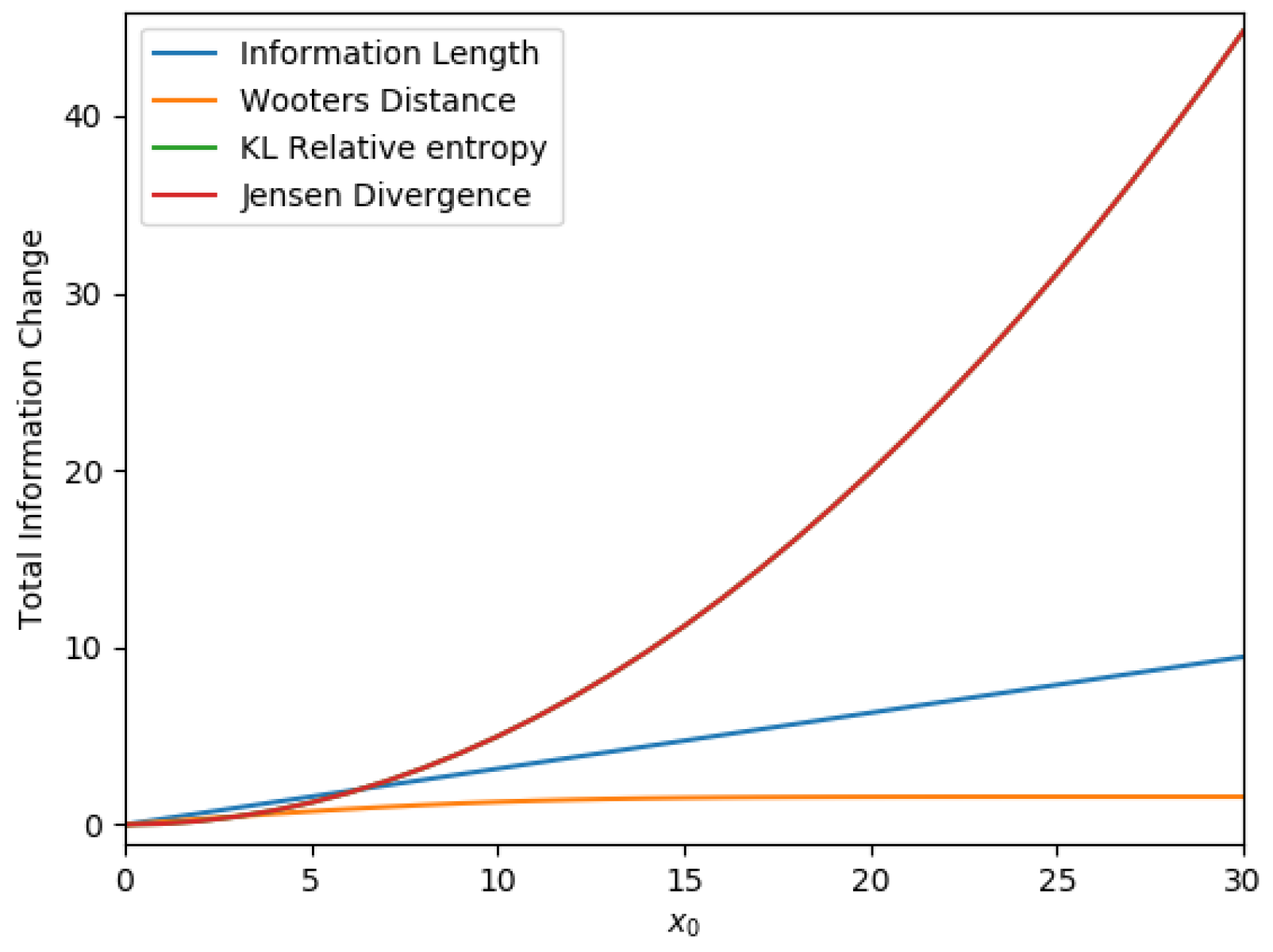
To elucidate the main difference between the distances in Equations (4)–(6) and Equation (13), we consider the relaxation problem by assuming . In the following, we compare the distance between and by using and in Equations (4)–(6) and Equation (13). Analytical expressions for these distances are given in [22].
Each curve in Figure 1 shows how each distance depends on the initial mean position . The four different curves are for (in blue), Wootters’ distance (in orange), K-L relative entropy (in green), and Jensen divergence (in red), respectively. The relative entropy and Jensen divergence exhibit similar behavior, the red and green color curves being superimposed on each other. Of note is a linear relation between and in Figure 1. Such linear relation is not seen in other distances. This means that the information length is a unique measure that manifests a linear geometry around its equilibrium point in a linear Gaussian process [28,30]. Note that for a nonlinear force f, has a power-law relation with for a sufficiently large [18,28]. These contrast with the behaviour in a chaotic system [16,28] where depends sensitively on the initial condition and abruptly changes with . Thus, the information length provides a useful tool to geometrically understand attractor structures in relaxation problems.
3.2. Correlation between Two Interacting Components
We next show that the information length is also useful in elucidating the correlation between two interacting species such as two competing components relaxing to the same equilibrium in the long time limit. Specifically, the two interacting components with the time-dependent PDFs and are coupled through the Dichotomous noise [110,111] (see Appendix B) and relax into the same equilibrium Gaussian PDF around in the long time limit. Here, is the total PDF. For the case considered below, satisfies the O-U process (see Appendix B for details). We choose the initial conditions where with zero initial mean value while takes an initial mean value . These are demonstrated in the cartoon figure, Figure 2a,c.
Although , at the intermediate time , evolves in time due to its coupling to and thus , as shown in Figure 2b. Consequently, calculated from monotonically increases to its asymptotic value until it reaches the equilibrium (see Figure A2 in [22] for time-evolution of from and ). On the other hand, with an initial mean value undergoes a different time evolution (unless ) until it reaches the equilibrium.
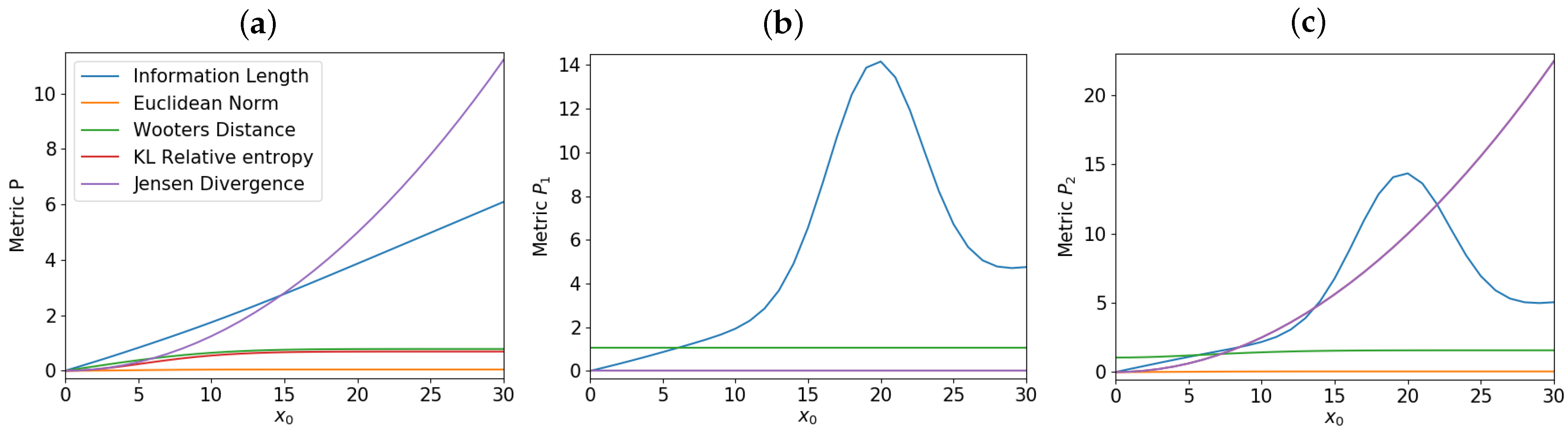
The distances in Equations (4)–(7) and Equation (13) can be calculated from the total , and for different values of . Results are shown in Figure 3a–c, respectively; (a) and , (b) and , and (c) and , respectively. Specifically, for each value of , we calculate the distances in Equations (4)–(7) and Equation (13) by using and for Figure 3a; and for Figure 3b; and for Figure 3c. The same procedure above is then repeated for many other ’s to show how each distance depends on .
For the total P, a linear relation between and is seen in Figure 3a (like in Figure 1). This linear relation is not seen in calculated from either or in Figure 3b or Figure 3c; a non-monotonic dependence of in Figure 3b,c is due to large-fluctuations and strong-correlation between and during time-evolution for large . What is quite remarkable is that in contrast to other distances, calculated from and in Figure 3b,c exhibits a very similar dependence on . It means that despite very different time-evolutions of and (see Figure 2), they undergo similar total change in information. These results suggest that strong coupling between two components can be inferred from their similar information length (see also [24,25]).
4. Thermodynamic Relations
To elucidate the utility of information geometric theory in understanding non-equilibrium thermodynamics, we review some of the important thermodynamic measures of irreversibility and dissipation [112] and relate them to information geometric measures and [29]. For illustration below, we use the model in Equations (14) and (15) unless stated otherwise. Corresponding to Equations (14) and (15) is the following Fokker-Planck equation [109]
where is the probability current.
4.1. Entropy Production Rate and Flow
For non-equilibrium thermodynamics, we need to consider the entropy in the system S and the environment , and the total entropy . To clarify the difference among these, we go over some derivation by using and to obtain
where,
Here, we used integration by parts in t and x. denotes the (total) entropy production rate, which is non-negative by definition, and serves as a measure of irreversibility [112]. The sign of in Equation (22) represents the direction in which the entropy flows between the system and environment. Specifically, () when the entropy flows from the system (environment) to the environment (system). is related to the heat flux from the system to the environment. The equality holds in an equilibrium reversible process. In this case, , which is the usual equilibrium thermodynamic relation. In comparison, when , .
For the O-U process with and in Equation (14), Equations (17)–(19) and Equations (21)–(22) lead to (see [29] for details)
Here, we used , , , , , and .
In order to relate these thermodynamical quantities and above to the information rate , we recall that for the O-U process [15,17,26,27,28],
Equations (24) and (27) then give us
Interestingly, Equation (28) reveals that the entropy production rate needs be normalized by variance . This is because of the extensive nature of unlike or . That is, changes its value when the variable x is rescaled by a scalar factor, say, () as . Furthermore, Equation (28) shows that the information rate in general does not have a simple relation to the entropy production rate (c.f., [107]).
One interesting limit of Equation (28) is the case of constant with . In that case, Equation (24) becomes while Equations (13), (27) and (28) give us
Equation (29) simply states that measures the total change in the mean value normalized by fluctuation level . Equation (30) manifests a linear relation between and when , as invoked in the previous works (e.g., [107]). Furthermore, a linear relation between and in Equation (30) implies that minimizing the entropy production along the trajectory corresponds to minimizing , which, in turn, is equivalent to minimizing (see Section 5 for further discussions).
Finally, to demonstrate how entropy production rate and thermal bath temperature (D) are linked to the speed of fluctuations [97], we rewrite Equation (28) as
For constant variance , Equation (31) gives a simple relation .
4.2. Non-Equilibrium Thermodynamical Laws
To relate the statistical measures in Section 4.1 to thermodynamics, we let U (internal energy) be the average potential energy and obtain (see also [66,113] and references therein)
where
The power represents the average rate at which the work is done to the system because of time-varying potential; the average work during the time interval is calculated by . On the other hand, represents the rate of dissipated heat.
Equation (32) establishes the non-equilibrium thermodynamic relation . Physically, it simply means that the work done to the system increases U while the dissipated heat to the environment decreases it. Equations (21), (32), and (34) permit us to define a non-equilibrium (information) free energy [92] and its time-derivative
where and . Since , Equation (35) leads to the following inequality
where the non-negative dissipated power (lost to the environment) is defined. Finally, the time-integral version of Equation (36) provides the bound on the average work performed on the system as (e.g., [68]).
4.3. Relative Entropy as a Measure of Irreversibility
The relative entropy has proven to be useful in understanding irreversibilities and non-equilibrium thermodynamic inequality relations [91,92,93,94,114,115,116]. In particular, the dissipated work (in Equation (36)) is related to the relative entropy between the PDFs in the forward and reverse processes
(e.g., see [91,92,93,94].) Here, and are the PDFs for the forward and reverse processes driven by the forward and reverse protocols, respectively. Using Equation (36) in Equation (37) immediately gives
which is a proxy for irreversibility (see [115,116] for a slightly different expression of Equation (38)). It is useful to note that forward and reversal protocols are also used to establish various fluctuations theorems for different dissipative measures such as entropy production, dissipated work, etc. (see, e.g., [80] for a nice review and references therein).
However, we cannot consider forward and reversal protocols in the absence of a model control parameter that can be prescribed as a function of time. Even in this case, the relative entropy is useful in quantifying irreversibility through inequalities, and this is what we focus on in the remainder of Section 4.3.
To this end, let us consider a non-equilibrium state which has an instantaneous non-equilibrium stationary state and calculate the relative entropy between the two. Here, is a steady solution of the Fokker-Planck equation in Equation (20) (e.g., see [29]). Specifically, one finds by treating the parameters to be constant (being frozen to their instantaneous values at a given time). Here, V and are the potential energy and the stationary free energy, respectively. For clarity, an example of is given in Section 4.4.
The average of in the non-equilibrium state can be expressed as follows:
Here, we used the fact the relative entropy is non-negative. Equation (40) explicitly shows that non-equilibrium free energy is bounded below by the stationary one (see also [1,92] and references therein for open Hamiltonian systems).
Here, , etc. The derivation of Equation (41) for open-driven Hamiltonian systems is provided in [92] (see their Equation (38)).
On the other hand, we directly calculate the time-derivative of in Equation (40) by using , , and , and :
4.4. Example
We consider with a constant u so that in Equation (14). While the discussion below explicitly involves , the results are general and valid for the limiting case . The case with is an example where the forward and reversal protocols do not exist while a non-equilibrium stationary state does.
For , Equation (19) is simplified as follows
For the non-equilibrium stationary state with fixed and D, is also constant (). Therefore, we have
Then, we can find (see [29] for details)
Here, we used Equations (23)–(26), and in Equations (44) and (18), respectively, and .
It is worth looking at the two interesting limits of Equations (46)–(50). First, in the long time limit as , the following simpler relations are found:
Equation (51) illustrates how the external force keeps the system out of equilibrium even in the long time limit, with non-zero entropy production and dissipation. When there is no external force , the system reaches equilibrium as , and all quantities in Equation (51) apart from become zero.
The second is when the system is initially in equilibrium with and and evolve in time as it is driven out of equilibrium by . As u does not affect variance, () and for all time. In this case, we find
Equation (52) shows that , , , , and start with zero values at and monotonically increase to their asymptotic values as .
5. Inequalities
Section 4 utilized the average (first moment) of a variable (e.g., ) and the average of its first time derivative () while the work is defined by the time integral of in Equation (33). This section aims to show that the rates at which average quantities vary with time are bounded by fluctuations and . Since the average and time derivatives do not commute, we pay particular attention to when the average is taken.
To this end, let us first define the microscopic free energy (called the chemical potential energy in [113]). In terms of , we have and . On the other hand,
means that the average rate of change in the microscopic free is the power. From Equation (54), it follows
Equation (55) establishes the relation between the microscopic free energy and .
Next, we calculate the time-derivative of
Using in Equation (56) gives in terms of as
Equation (57) is to be used in Section 5.1 for linking to through an inequality.
5.1. General Inequality Relations
Equation (60) (Equation (59)) establishes the inequality between entropy production rate (heat flux) and the product of the RMS fluctuations of the microscopic free energy (potential energy) and . Since , we have
These relations are to be used in Section 5.2 below.
5.2. Applications to the Non-Autonomous O-U Process
For a linear O-U process with and in Equation (14), we use , and to show
6. Geodesics, Control and Hyperbolic Geometry
The section aims to discuss geodesics in information geometry and its implications for self-organization and control. To illustrate the key concepts, we utilize an analytically solvable, generalized O-U process given by
where is a damping constant; is a deterministic force which determines the time evolution of the mean value of x; is a short (delta)-correlated noise with the time-dependent amplitude in general, satisfying Equation (15).
6.1. Geodesics–Shortest-Distance Path
A geodesics between the two spatial locations is a unique path with the shortest distance. A similar concept can be applied to information geometry to define a unique evolution path between the two given PDFs, say, and in the statistical space. The Wootters’ distance in quantum mechanics in Equation (4) is such an example. For time-varying stochastic processes, there is an infinite number of different trajectories between the two PDFs at different times. The key question that we address in this section is how to find an exact time evolution of when initial and final PDFs [15] are given. This is a much more difficult problem than finding a minimum distance between two PDFs (like the Wootter’s distance). In the following, we sketch some main steps needed for finding such a unique evolution path (the so-called geodesics) between given initial and final PDFs by minimizing (see [15] for detailed steps).
For the O-U process in Equation (64), a geodesic solution does not exist for constant , and D. Thus, finding a geodesic solution boils down to determing suitable functions of , or [15]. To be specific, let and , respectively, be the PDFs at the time and () and find a geodesic solution by minimizing . The latter is equivalent to minimizing and to keeping constant. (This geodesics is also called an optimal path (e.g., see [107]).) We rewrite in Equation (27) for the O-U process in terms of
The Euler-Lagrange equation
( and ) then gives us
where c is constant. An alternative method of obtaining Equations (69) and (70) is provided in Appendix C. The following equations are obtained from Equations (69) and (70) [15]
where is another (integration) constant. General solutions to Equations (70) and (71) for were found in terms of hyperbolic functions as [15]
where A and B are constant.
Equation (73) can be rewritten using and as follows
where s denotes the sign of c so that when while when . Equation (74) is an equation of a circle for the variables z and with the radius R and the center , defined in the upper-half plane where . Thus, geodesic motions occur along the portions of a circle as long as (as can be seen in Figure 4). A geodesic moves on a circle with a larger radius for a larger information rate and speed and vice versus. This manifests the hyperbolic geometry in the upper half Poincaré model [13,117] where the half-plane represents z and (see also Appendix D). The constants , and B determine the coordinate of the center and the radius of the circle R. These constants should be fixed by the fixed conditions at the initial and final time .
Having found the most general form of the geodesic solution for and , the next steps require finding the values of constant values to satisfy the boundary conditions at and , and then finding appropriate , , and that ensure the geodesic solutions. This means the O-U process should be controlled by , and to ensure a geodesic solution.
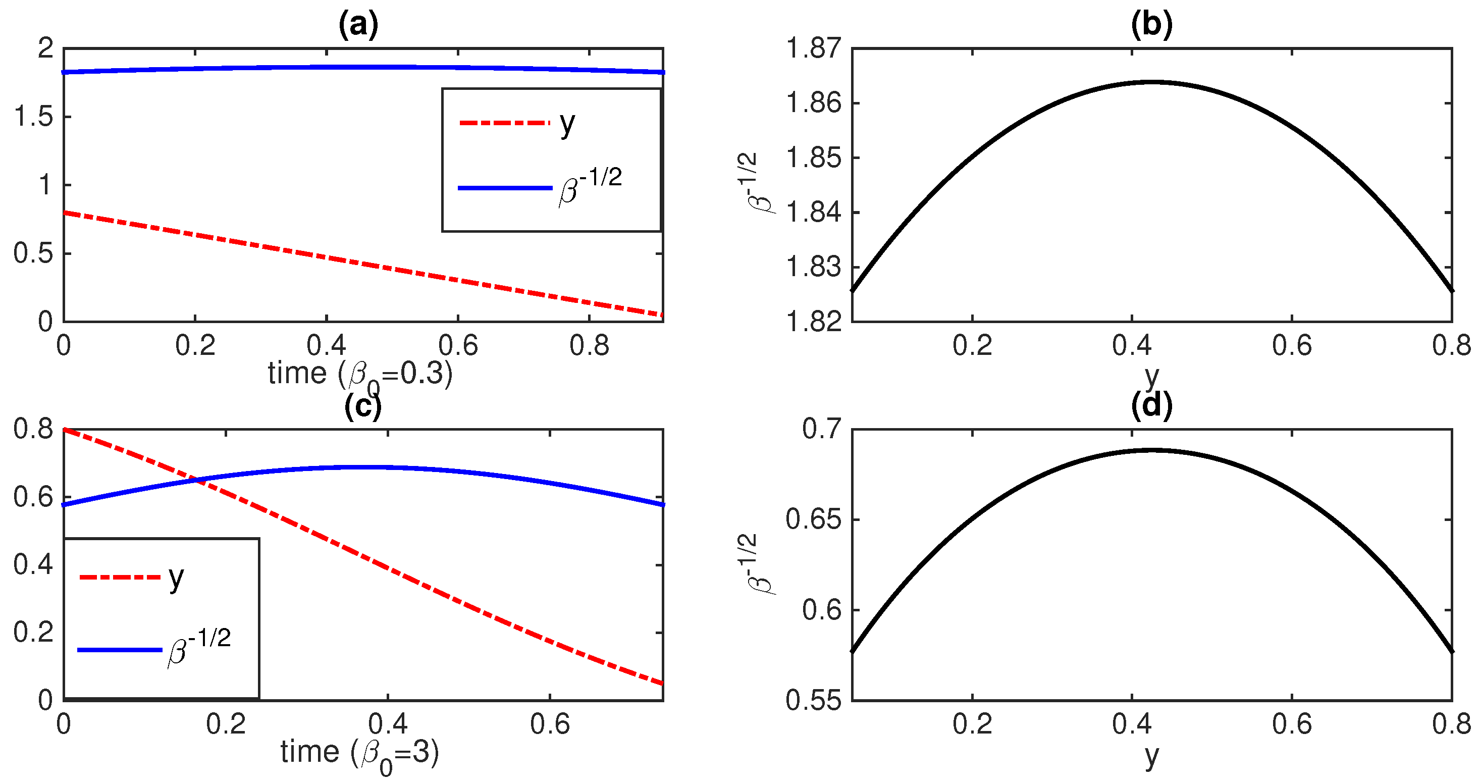
Figure 4 shows an example of a geodesic solution in the upper half-plane y and when is constant while and are time-dependent. The boundary conditions are chosen as and in all panels (a)–(d). in panels (a) and (b) while in panels (c) and (d). Interestingly, circular-shape phase-portraits are seen in panels (b) and (d), reflecting hyperbolic geometry noted above (see also Appendix D) [13,117]. The speed at which the geodesic motion takes place in the phase portrait is determined by the constant value of (i.e., the larger , the faster time evolution).
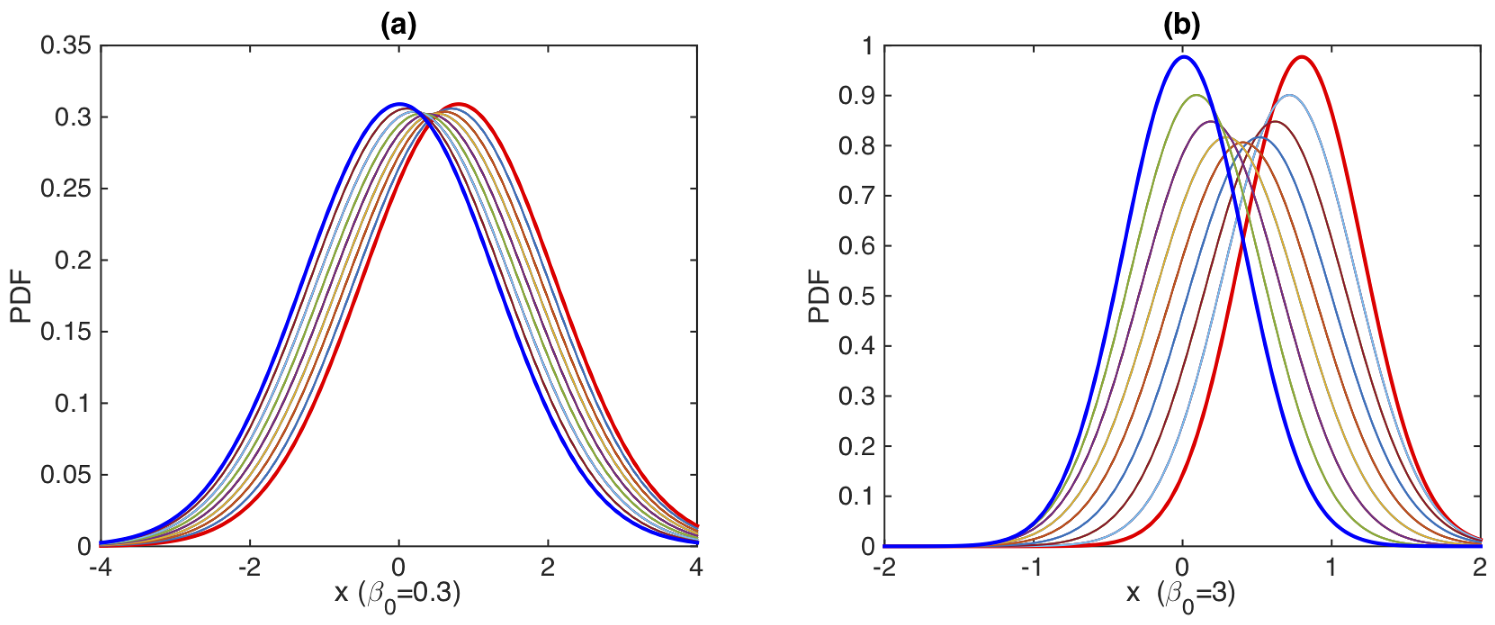
Figure 5a,b are the corresponding PDF snapshots at different times (shown in different colors), demonstrating how the PDF evolves from the initial PDF in red to the final PDF in blue. In both cases, it is prominent that the PDF width () initially broadens and then becomes narrower.
6.2. Comments on Self-Organization and Control
Self-organization (also called homeostasis) is the novel phenomena where order spontaneously emerges out of disorder and is maintained by different feedbacks in complex systems [45,52,53,118,119,120,121,122,123]. The extremum principles of thermodynamics such as the minimum entropy production (e.g., [119,121]) or maximum entropy entropy production (e.g., [122,123]) have been proposed by considering a steady state or an instant time in different problems.
However, far from equilibrium, self-organization can be a time-varying non-equilibrium process involving perpetual or large fluctuations (e.g., see [52,53,54]). In this case, the extreme of entropy production should be on accumulative entropy production over time rather than at one instant time nor in a steady state. That is, we should consider the time-integral of the entropy production , or equivalently, the time-integral of . As seen from Equations (24) and (53), for a linear O-U process with a constant variance, there is an exact proportionality between and . In this case, the extreme of would be the same as the extreme of . However, as noted previously, does not hold in general (e.g., see Equation (28)).
With these comments, we now look at the implications of a geodesic for self-organization, in particular, in biosystems. For the very existence and optimal functions of a living organiss, it is critical to minimize the dispersion of its physical states and to maintain its states within certain bounds upon changing conditions [124]. How fast its state changes in time can be quantified by the surprise rate . Since , we use its RMS value (see Equation (9)) and realize that the total change over a finite time interval is nothing more than . Thus, minimizing the accumulative/time-integral of the RMS surprise rate is equivalent to minimizing . Envisioning surprise rate as biological cost associated with changes (e.g., needed in updating the future prediction based on the current state [124,125]), we can then interpret as an accumulative biological cost. Thus, geodesic would be an optimal path that minimizes such an accumulative biological cost.
Ref [15] addressed how to utilize this idea to control populations (tumors). Specifically, the results in Section 6.1 were applied to a nonlinear stochastic growth model (obtained by a nonlinear change of variables of the O-U process), and the geodesic solution in Equation (73) was used to find the optimal protocols and in reducing a large-size tumor to a smaller one. Here, in this problem, represents the heterogeneity of tumor cells (e.g., larger D for metastatic tumor) that can be controlled by gene reprogramming while models the effect of a drug or radiation that reduces the mean tumor population/size.
7. Discussions and Conclusions
There has been a growing interest in information geometry from theoretical and practical considerations. This paper discussed some recent developments in information geometric theory, focusing on time-dependent dynamic aspects of non-equilibrium processes (e.g., time-varying mean value, time-varying variance, or temperature) and their thermodynamic and physical/biological implications.
In Section 2 and Section 3, by utilizing a Langevin model of an over-damped stochastic process , we highlighted the importance of a path-dependent distance in describing time-varying processes. In Section 4 and Section 5, we elucidated the thermodynamic meanings of the relative entropy and the information rate by relating them to the entropy production rate (), , heat flux (), dissipated work (), etc., and demonstrated the role of in determining bounds (or speed limit) on thermodynamical quantities.
Specifically, in the O-U process, we showed the exact relation (Equation (28)), which is simplified as when ( is the standard deviation of x). Finally, Section 6 discussed geodesic and its implication for self-organization as well as the underlying hyperbolic geometry. It remains future works to explore the link between and the entropy production rate in other (e.g., nonlinear) systems consisting of three or more interacting components or data from self-organizing systems (e.g., normal brain).
Funding
This research received no funding.
Data Availability Statement
Data are available from the author.
Acknowledgments
Eun-jin Kim acknowledges the Leverhulme Trust Research Fellowship (RF- 2018-142-9) and thanks the collaborators, especially, James Heseltine who contributed to the works in this paper.
Conflicts of Interest
The author declares no conflict of interest.
Appendix A
In this Appendix, we show the invariance of Equation (9) when x changes as . Using the conservation of the probability, we then have
Since is independent of time t, it follows that . Using this and , we have
This shows that and give the same .
Appendix B. The Coupled O-U Process
Here, D is the strength of a short-correlated Gaussian noise given by Equation (15). These equations are the coupled O-U processes with the coupling constants and through the Dichotomous noise [110,111].
For simplicity, we use and and the following initial conditions
The solutions are given by
where
for . In the limit of , and in Equations (A7) and (A8) approach the same equilibrium distribution
where . We note that the total PDF satisfies the single O-U process where the initial PDF is given by the sum of Equations (A5) and (A6).
Figure 3 is shown for the fixed parameter values , and , . Different values of the initial mean position of are used to examine how metrics depend on . As noted in Section 2.2, at is chosen to be the same as the final equilibrium state which has the zero mean value and inverse temperature .
Appendix C. Curved Geometry: The Christoffel and Ricci-Curvature Tensors
A geodesic solution in Section 6.1 can also be found by solving the geodesic equation in general relativity (e.g., [31,107]). To this end, we let the two parameters be and and express Equation (A11) in terms of the metric tensor as follows (see also Equation (10))
where
Note that while is diagonal, the 1-st diagonal component depends on (the second parameter). That is, is not independent of j-th parameter for in general. From Equation (A12), we can find non-zero components of connection tensor ()
A geodesic equation in terms of the Christoffel tensors becomes
Equations (A13)–(A15) give Equation (70). Note that if is independent of the () for all i and j, the Christoffel tensors have non-zero values only for , leading to a much simpler geodesic solution (e.g., see [31]).
Finally, to appreciate the curved geometry associated with this geodesic solution, we proceed to calculate the Riemann curvature tensor and the Ricci tensor from Equation (A13) and find the following non-zero components [15]
Non-zero curvature tensors represent that the metric space is curved with a finite curvature. Specifically, we find the Ricci tensor and curvature R:
The negative curvature is typical of hyperbolic geometry. Finally, using , we calculate the Einstein field equation
Since where is the stress-energy tensor, we see that for this problem.
Appendix D. Hyperbolic Geometry
References
- Cover, T.M.; Thomas, J.A. Elements of Information Theory; Wiley: New York, NY, USA, 1991. [Google Scholar]
- Parr, T.; Da Costa, L.; Friston, K.J. Markov blankets, information geometry and stochastic thermodynamics. Philos. Trans. R. Soc. A 2019, 378, 20190159. [Google Scholar] [CrossRef] [PubMed] [Green Version]
- Oizumi, M.; Tsuchiya, N.; Amari, S. Unified framework for information integration based on information geometry. Proc. Nat. Am. Soc. 2016, 113, 14817. [Google Scholar] [CrossRef] [PubMed] [Green Version]
- Kowalski, A.M.; Martin, M.T.; Plastino, A.; Rosso, O.A.; Casas, M. Distances in Probability Space and the Statistical Complexity Setup. Entropy 2011, 13, 1055–1075. [Google Scholar] [CrossRef] [Green Version]
- Martin, M.T.; Plastino, A.; Rosso, O.A. Statistical complexity and disequilibrium. Phys. Lett. A 2003, 311, 126–132. [Google Scholar] [CrossRef]
- Gibbs, A.L.; Su, F.E. On choosing and bounding probability metrics. Int. Stat. Rev. 2002, 70, 419–435. [Google Scholar] [CrossRef] [Green Version]
- Jordan, R.; Kinderlehrer, D.; Otto, F. The variational formulation of the Fokker–Planck equation. SIAM J. Math. Anal. 1998, 29, 1–17. [Google Scholar] [CrossRef]
- Takatsu, A. Wasserstein geometry of Gaussian measures. Osaka J. Math. 2011, 48, 1005–1026. [Google Scholar]
- Lott, J. Some geometric calculations on Wasserstein space. Commun. Math. Phys. 2008, 277, 423–437. [Google Scholar] [CrossRef] [Green Version]
- Gangbo, W.; McCann, R.J. The geometry of optimal transportation. Acta Math. 1996, 177, 113–161. [Google Scholar] [CrossRef]
- Zamir, R. A proof of the Fisher information inequality via a data processing argument. IEEE Trans. Inf. Theory 1998, 44, 1246–1250. [Google Scholar] [CrossRef]
- Otto, F.; Villani, C. Generalization of an Inequality by Talagrand and Links with the Logarithmic Sobolev Inequality. J. Funct. Anal. 2000, 173, 361–400. [Google Scholar] [CrossRef] [Green Version]
- Costa, S.; Santos, S.; Strapasson, J. Fisher information distance. Discrete Appl. Math. 2015, 197, 59–69. [Google Scholar] [CrossRef]
- Ferradans, S.; Xia, G.-S.; Peyré, G.; Aujol, J.-F. Static and dynamic texture mixing using optimal transport. Lecture Notes Comp. Sci. 2013, 7893, 137–148. [Google Scholar]
- Kim, E.; Lee, U.; Heseltine, J.; Hollerbach, R. Geometric structure and geodesic in a solvable model of nonequilibrium process. Phys. Rev. E 2016, 93, 062127. [Google Scholar] [CrossRef] [PubMed] [Green Version]
- Nicholson, S.B.; Kim, E. Investigation of the statistical distance to reach stationary distributions. Phys. Lett. A 2015, 379, 83–88. [Google Scholar] [CrossRef]
- Heseltine, J.; Kim, E. Novel mapping in non-equilibrium stochastic processes. J. Phys. A 2016, 49, 175002. [Google Scholar] [CrossRef]
- Kim, E.; Hollerbach, R. Signature of nonlinear damping in geometric structure of a nonequilibrium process. Phys. Rev. E 2017, 95, 022137. [Google Scholar] [CrossRef] [PubMed] [Green Version]
- Kim, E.; Hollerbach, R. Geometric structure and information change in phase transitions. Phys. Rev. E 2017, 95, 062107. [Google Scholar] [CrossRef] [Green Version]
- Kim, E.; Jacquet, Q.; Hollerbach, R. Information geometry in a reduced model of self-organised shear flows without the uniform coloured noise approximation. J. Stat. Mech. 2019, 2019, 023204. [Google Scholar] [CrossRef] [Green Version]
- Anderson, J.; Kim, E.; Hnat, B.; Rafiq, T. Elucidating plasma dynamics in Hasegawa-Wakatani turbulence by information geometry. Phys. Plasmas 2020, 27, 022307. [Google Scholar] [CrossRef]
- Heseltine, J.; Kim, E. Comparing information metrics for a coupled Ornstein-Uhlenbeck process. Entropy 2019, 21, 775. [Google Scholar] [CrossRef] [PubMed] [Green Version]
- Kim, E.; Heseltine, J.; Liu, H. Information length as a useful index to understand variability in the global circulation. Mathematics 2020, 8, 299. [Google Scholar] [CrossRef] [Green Version]
- Kim, E.; Hollerbach, R. Time-dependent probability density functions and information geometry of the low-to-high confinement transition in fusion plasma. Phys. Rev. Res. 2020, 2, 023077. [Google Scholar] [CrossRef] [Green Version]
- Hollerbach, R.; Kim, E.; Schmitz, L. Time-dependent probability density functions and information diagnostics in forward and backward processes in a stochastic prey-predator model of fusion plasmas. Phys. Plasmas 2020, 27, 102301. [Google Scholar] [CrossRef]
- Guel-Cortez, A.J.; Kim, E. Information Length Analysis of Linear Autonomous Stochastic Processes. Entropy 2020, 22, 1265. [Google Scholar] [CrossRef] [PubMed]
- Guel-Cortez, A.J.; Kim, E. Information geometric theory in the prediction of abrupt changes in system dynamics. Entropy 2021, 23, 694. [Google Scholar] [CrossRef]
- Kim, E. Investigating Information Geometry in Classical and Quantum Systems through Information Length. Entropy 2018, 20, 574. [Google Scholar] [CrossRef] [Green Version]
- Kim, E. Information geometry and non-equilibrium thermodynamic relations in the over-damped stochastic processes. J. Stat. Mech. Theory Exp. 2021, 2021, 093406. [Google Scholar] [CrossRef]
- Parr, T.; Da Costa, L.; Heins, C.; Ramstead, M.J.D.; Friston, K.J. Memory and Markov Blankets. Entropy 2021, 23, 1105. [Google Scholar] [CrossRef]
- Da Costa, L.; Thomas, P.; Biswa, S.; Karl, F.J. Neural Dynamics under Active Inference: Plausibility and Efficiency of Information Processing. Entropy 2021, 23, 454. [Google Scholar] [CrossRef]
- Frieden, B.R. Science from Fisher Information; Cambridge University Press: Cambridge, UK, 2004. [Google Scholar]
- Wootters, W. Statistical distance and Hilbert-space. Phys. Rev. D 1981, 23, 357–362. [Google Scholar] [CrossRef]
- Ruppeiner, G. Thermodynamics: A Riemannian geometric model. Phys. Rev. A. 1079, 20, 1608. [Google Scholar] [CrossRef]
- Salamon, P.; Nulton, J.D.; Berry, R.S. Length in statistical thermodynamics. J. Chem. Phys. 1985, 82, 2433–2436. [Google Scholar] [CrossRef]
- Nulton, J.; Salamon, P.; Andresen, B.; Anmin, Q. Quasistatic processes as step equilibrations. J Chem. Phys. 1985, 83, 334. [Google Scholar] [CrossRef]
- Braunstein, S.L.; Caves, C.M. Statistical distance and the geometry of quantum states. Phys. Rev. Lett. 1994, 72, 3439. [Google Scholar] [CrossRef]
- Diósi, L.; Kulacsy, K.; Lukács, B.; Rácz, A. Thermodynamic length, time, speed, and optimum path to minimize entropy production. J. Chem. Phys. 1996, 105, 11220. [Google Scholar] [CrossRef] [Green Version]
- Crooks, G.E. Measuring thermodynamic length. Phys. Rev. Lett. 2007, 99, 100602. [Google Scholar] [CrossRef] [Green Version]
- Salamon, P.; Nulton, J.D.; Siragusa, G.; Limon, A.; Bedeaus, D.; Kjelstrup, D. A Simple Example of Control to Minimize Entropy Production. J. Non-Equilib. Thermodyn. 2002, 27, 45–55. [Google Scholar] [CrossRef]
- Feng, E.H.; Crooks, G.E. Far-from-equilibrium measurements of thermodynamic length. Phys. Rev. E. 2009, 79, 012104. [Google Scholar] [CrossRef] [Green Version]
- Sivak, D.A.; Crooks, G.E. Thermodynamic Metrics and Optimal Paths. Phys. Rev. Lett. 2012, 8, 190602. [Google Scholar] [CrossRef] [PubMed] [Green Version]
- Matey, A.; Lamberti, P.W.; Martin, M.T.; Plastron, A. Wortters’ distance resisted: A new distinguishability criterium. Eur. Rhys. J. D 2005, 32, 413–419. [Google Scholar]
- d’Onofrio, A. Fractal growth of tumors and other cellular populations: Linking the mechanistic to the phenomenological modeling and vice versa. Chaos Solitons Fractals 2009, 41, 875. [Google Scholar] [CrossRef] [Green Version]
- Newton, A.P.L.; Kim, E.; Liu, H.-L. On the self-organizing process of large scale shear flows. Phys. Plasmas 2013, 20, 092306. [Google Scholar] [CrossRef]
- Kim, E.; Liu, H.-L.; Anderson, J. Probability distribution function for self-organization of shear flows. Phys. Plasmas 2009, 16, 0552304. [Google Scholar] [CrossRef] [Green Version]
- Kim, E.; Diamond, P.H. Zonal flows and transient dynamics of the L-H transition. Phys. Rev. Lett. 2003, 90, 185006. [Google Scholar] [CrossRef] [PubMed] [Green Version]
- Feinberg, A.P.; Irizarry, R.A. Stochastic epigenetic variation as a driving force of development, evolutionary adaptation, and disease. Proc. Natl. Acad. Sci. USA 2010, 107, 1757. [Google Scholar] [CrossRef] [PubMed] [Green Version]
- Wang, N.X.; Zhang, X.M.; Han, X.B. The effects of environmental disturbances on tumor growth. Braz. J. Phys. 2012, 42, 253. [Google Scholar] [CrossRef] [Green Version]
- Lee, J.; Farquhar, K.S.; Yun, J.; Frankenberger, C.; Bevilacqua, E.; Yeung, E.; Kim, E.; Balázsi, G.; Rosner, M.R. Network of mutually repressive metastasis regulators can promote cell heterogeneity and metastatic transitions. Proc. Natl. Acad. Sci. USA 2014, 111, E364. [Google Scholar] [CrossRef] [PubMed] [Green Version]
- Lee, U.; Skinner, J.J.; Reinitz, J.; Rosner, M.R.; Kim, E. Noise-driven phenotypic heterogeneity with finite correlation time. PLoS ONE 2015, 10, e0132397. [Google Scholar]
- Haken, H. Information and Self-Organization: A Macroscopic Approach to Complex Systems, 3rd ed.; Springer: Berlin/Heidelberg, Germany, 2006; pp. 63–64. [Google Scholar]
- Kim, E. Intermittency and self-organisation in turbulence and statistical mechanics. Entropy 2019, 21, 574. [Google Scholar] [CrossRef] [Green Version]
- Aschwanden, M.J.; Crosby, N.B.; Dimitropoulou, M.; Georgoulis, M.K.; Hergarten, S.; McAteer, J.; Milovanov, A.V.; Mineshige, S.; Morales, L.; Nishizuka, N.; et al. 25 Years of Self-Organized Criticality: Solar and Astrophysics. Space Sci. Rev. 2016, 198, 47–166. [Google Scholar] [CrossRef] [Green Version]
- Zweben, S.J.; Boedo, J.A.; Grulke, O.; Hidalgo, C.; LaBombard, B.; Maqueda, R.J.; Scarin, P.; Terry, J.L. Edge turbulence measurements in toroidal fusion devices. Plasma Phys. Contr. Fusion 2007, 49, S1–S23. [Google Scholar] [CrossRef]
- Politzer, P.A. Observation of avalanche-like phenomena in a magnetically confined plasma. Phys. Rev. Lett. 2000, 84, 1192–1195. [Google Scholar] [CrossRef] [PubMed]
- Beyer, P.; Benkadda, S.; Garbet, X.; Diamond, P.H. Nondiffusive transport in tokamaks: Three-dimensional structure of bursts and the role of zonal flows. Phys. Rev. Lett. 2000, 85, 4892–4895. [Google Scholar] [CrossRef] [Green Version]
- Drake, J.F.; Guzdar, P.N.; Hassam, A.B. Streamer formation in plasma with a temperature gradient. Phys. Rev. Lett. 1988, 61, 2205–2208. [Google Scholar] [CrossRef]
- Antar, G.Y.; Krasheninnikov, S.I.; Devynck, P.; Doerner, R.P.; Hollmann, E.M.; Boedo, J.A.; Luckhardt, S.C.; Conn, R.W. Experimental evidence of intermittent convection in the edge of magnetic confinement devices. Phys. Rev. Lett. 2001, 87, 065001. [Google Scholar] [CrossRef] [Green Version]
- Carreras, B.A.; Hidalgo, E.; Sanchez, E.; Pedrosa, M.A.; Balbin, R.; Garcia-Cortes, I.; van Milligen, B.; Newman, D.E.; Lynch, V.E. Fluctuation-induced flux at the plasma edge in toroidal devices. Phys. Plasmas 1996, 3, 2664–2672. [Google Scholar] [CrossRef]
- De Vries, P.C.; Johnson, M.F.; Alper, B.; Buratti, P.; Hender, T.C.; Koslowski, H.R.; Riccardo, V. JET-EFDA Contributors, Survey of disruption causes at JET. Nuclear Fusion 2011, 51, 053018. [Google Scholar] [CrossRef]
- Kates-Harbeck, J.; Svyatkovskiy, A.; Tang, W. Predicting disruptive instabilities in controlled fusion plasmas through deep learning. Nature 2019, 568, 527. [Google Scholar] [CrossRef]
- Landau, L.; Lifshitz, E.M. Statistical Physics: Part 1. In Course of Theoretical Physics; Elsevier Ltd.: New York, NY, USA, 1980; Volume 5. [Google Scholar]
- Shannon, C.E. A Mathematical Theory of Communication. Bell Syst. Tech. J. 1948, 27, 623. [Google Scholar] [CrossRef]
- Jarzynski, C.R. Equalities and Inequalities: Irreversibility and the Second Law of Thermodynamics at the Nanoscale. Annu. Rev. Condens. Matter Phys. 2011, 2, 329–351. [Google Scholar] [CrossRef] [Green Version]
- Sekimoto, K. Stochastic Energetic; Lecture Notes in Physics 799; Springer: Heidelberg, Germany, 2010. [Google Scholar] [CrossRef]
- Jarzynski, C.R. Comparison of far-from-equilibrium work relations. Physique 2007, 8, 495–506. [Google Scholar] [CrossRef] [Green Version]
- Jarzynski, C.R. Nonequilibrium Equality for Free Energy Differences. Phys. Rev. Lett. 1997, 78, 2690–2693. [Google Scholar] [CrossRef] [Green Version]
- Evans, D.J.; Cohen, G.D.; Morriss, G.P. Probability of Second Law Violations in Shearing Steady States. Phys. Rev. Lett. 1993, 71, 2401. [Google Scholar] [CrossRef] [Green Version]
- Evans, D.J.; Searles, D.J. The Fluctuation Theorem. Adv. Phys. 2012, 51, 1529–1585. [Google Scholar] [CrossRef]
- Gallavotti, G.; Cohen, E.G.D. Dynamical Ensembles in Nonequilibrium Statistical Mechanics. Phys. Rev. Lett. 1995, 74, 2694. [Google Scholar] [CrossRef] [Green Version]
- Kurchan, J. Fluctuation theorem for stochastic dynamics. J. Phys. A Math. Gen. 1998, 31, 3719. [Google Scholar] [CrossRef] [Green Version]
- Searles, D.J.; Evans, D.J. Ensemble dependence of the transient fluctuation theorem. J. Chem. Phys. 2000, 13, 3503. [Google Scholar] [CrossRef] [Green Version]
- Seifert, U. Entropy production along a stochastic trajectory and an integral fluctuation theorem. Phys. Rev. Lett. 2005, 95, 040602. [Google Scholar] [CrossRef] [PubMed] [Green Version]
- Abreu, D.; Seifert, U. Extracting work from a single heat bath through feedback. EuroPhys. Lett. 2011, 94, 10001. [Google Scholar] [CrossRef]
- Seifert, U. Stochastic thermodynamics, fluctuation theorems and molecular machines. Rep. Prog. Phys. 2012, 75, 26001. [Google Scholar] [CrossRef] [Green Version]
- Spinney, R.E.; Ford, I.J. Fluctuation relations: A pedagogical overview. arXiv 2012, arXiv:1201.6381S. [Google Scholar]
- Haas, K.R.; Yang, H.; Chu, J.-W. Trajectory Entropy of Continuous Stochastic Processes at Equilibrium. J. Phys. Chem. Lett. 2014, 5, 999. [Google Scholar] [CrossRef]
- Van den Broeck, C. Stochastic thermodynamics: A brief introduction. Phys. Complex Colloids 2013, 184, 155–193. [Google Scholar]
- Murashita, Y. Absolute Irreversibility in Information Thermodynamics. arXiv 2015, arXiv:1506.04470. [Google Scholar]
- Tomé, T. Entropy Production in Nonequilibrium Systems Described by a Fokker-Planck Equation. Braz. J. Phys. 2016, 36, 1285–1289. [Google Scholar] [CrossRef] [Green Version]
- Salazar, D.S.P. Work distribution in thermal processes. Phys. Rev. E 2020, 101, 030101. [Google Scholar] [CrossRef] [PubMed] [Green Version]
- Kullback, S. Letter to the Editor: The Kullback-Leibler distance. Am. Stat. 1951, 41, 340–341. [Google Scholar]
- Sagawa, T. Thermodynamics of Information Processing in Small Systems; Springer: Berlin/Heidelberg, Germany, 2012. [Google Scholar]
- Nielsen, M.A.; Chuang, I.L. Quantum Computation and Quantum Information; Cambridge University Press: Cambridge, UK, 2000. [Google Scholar]
- Landauer, R. Irreversibility and heat generation in the computing process. IBM J. Res. Dev. 1961, 5, 183–191. [Google Scholar] [CrossRef]
- Bérut, A.; Arakelyan, A.; Petrosyan, A.; Ciliberto, S.; Dillenschneider, R.; Lutz, E. Experimental verification of Landauer’s principle linking information and thermodynamics. Nature 2012, 483, 187. [Google Scholar] [CrossRef]
- Leff, H.S.; Rex, A.F. Maxwell’s Demon: Entropy, Information, Computing; Princeton University Press: Princeton, NJ, USA, 1990. [Google Scholar]
- Bekenstein, J.D. How does the entropy/information bound work? Found. Phys. 2005, 35, 1805. [Google Scholar] [CrossRef] [Green Version]
- Capozziello, S.; Luongo, O. Information entropy and dark energy evolution. Int. J. Mod. Phys. D 2018, 27, 1850029. [Google Scholar] [CrossRef] [Green Version]
- Kawai, R.; Parrondo, J.M.R.; Van den Broeck, C. Dissipation: The phase-space perspective. Phys. Rev. Lett. 2007, 98, 080602. [Google Scholar] [CrossRef] [PubMed] [Green Version]
- Esposito, M.; Van den Broeck, C. Second law and Landauer principle far from equilibrium. Europhys. Lett. 2011, 95, 40004. [Google Scholar] [CrossRef] [Green Version]
- Horowitz, J.; Jarzynski, C.R. An illustrative example of the relationship between dissipation and relative entropy. Phys. Rev. E 2009, 79, 021106. [Google Scholar] [CrossRef] [PubMed] [Green Version]
- Parrondo, J.M.R.; van den Broeck, C.; Kawai, R. Entropy production and the arrow of time. New J. Phys. 2009, 11, 073008. [Google Scholar] [CrossRef]
- Deffner, S.; Lutz, E. Information free energy for nonequilibrium states. arXiv 2012, arXiv:1201.3888. [Google Scholar]
- Horowitz, J.M.; Sandberg, H. Second-law-like inequalities with information and their interpretations. New J. Phys. 2014, 16, 125007. [Google Scholar] [CrossRef]
- Nicholson, S.B.; García-Pintos, L.P.; del Campo, A.; Green, J.R. Time-information uncertainty relations in thermodynamics. Nat. Phys. 2020, 16, 1211–1215. [Google Scholar] [CrossRef]
- Flego, S.P.; Frieden, B.R.; Plastino, A.; Plastino, A.R.; Soffer, B.H. Nonequilibrium thermodynamics and Fisher information: Sound wave propagation in a dilute gas. Phys. Rev. E 2003, 68, 016105. [Google Scholar] [CrossRef]
- Carollo, A.; Spagnolo, B.; Dubkov, A.A.; Valenti, D. On quantumness in multi-parameter quantum estimation. J. Stat. Mech. Theory E 2019, 2019, 094010. [Google Scholar] [CrossRef] [Green Version]
- Carollo, A.; Valenti, D.; Spagnolo, B. Geometry of quantum phase transitions. Phys. Rep. 2020, 838, 1–72. [Google Scholar] [CrossRef] [Green Version]
- Davies, P. Does new physics lurk inside living matter? Phys. Today 2020, 73, 34. [Google Scholar] [CrossRef]
- Sjöqvist, E. Geometry along evolution of mixed quantum states. Phys. Rev. Res. 2020, 2, 013344. [Google Scholar] [CrossRef] [Green Version]
- Briët, J.; Harremoës, P. Properties of classical and quantum Jensen-Shannon divergence. Phys. Rev. A 2009, 79, 052311. [Google Scholar] [CrossRef] [Green Version]
- Casas, M.; Lambertim, P.; Lamberti, P.; Plastino, A.; Plastino, A.R. Jensen-Shannon divergence, Fisher information, and Wootters’ hypothesis. arXiv 2004, arXiv:quant-ph/0407147. [Google Scholar]
- Sánchez-Moreno, P.; Zarzo, A.; Dehesa, J.S. Jensen divergence based on Fisher’s information. J. Phys. A Math. Theor. 2012, 45, 125305. [Google Scholar] [CrossRef] [Green Version]
- López-Ruiz, L.; Mancini, H.; Calbet, X. A statistical measure of complexity. Phys. Lett. A 1995, 209, 321–326. [Google Scholar] [CrossRef] [Green Version]
- Cafaro, C.; Alsing, P.M. Information geometry aspects of minimum entropy production paths from quantum mechanical evolutions. Phys. Rev. E 2020, 101, 022110. [Google Scholar] [CrossRef] [Green Version]
- Ashida, K.; Oka, K. Stochastic thermodynamic limit on E. coli adaptation by information geometric approach. Biochem. Biophys. Res. Commun. 2019, 508, 690–694. [Google Scholar] [CrossRef] [Green Version]
- Risken, H. The Fokker-Planck Equation: Methods of Solution and Applications; Springer: Berlin, Germany, 1996. [Google Scholar]
- Van Den Brock, C. On the relation between white shot noise, Gaussian white noise, and the dichotomic Markov process. J. Stat. Phys. 1983, 31, 467–483. [Google Scholar] [CrossRef]
- Bena, I. Dichotomous Markov Noise: Exact results for out-of-equilibrium systems (a brief overview). Int. J. Mod. Phys. B 2006, 20, 2825–2888. [Google Scholar] [CrossRef] [Green Version]
- Onsager, L.; Machlup, S. Fluctuations and Irreversible Processes. Phys. Rev. 1953, 91, 1505–1512. [Google Scholar] [CrossRef]
- Parrondo, J.M.R.; de Cisneros, B.J.; Brito, R. Thermodynamics of Isothermal Brownian Motors. In Stochastic Processes in Physics, Chemistry, and Biology; Freund, J.A., Pöschel, T., Eds.; Lecture Notes in Physics; Springer: Berlin/Heidelberg, Germany, 2000; Volume 557. [Google Scholar] [CrossRef]
- Gaveau, B.; Granger, L.; Moreau, M.; Schulman, L. Dissipation, interaction, and relative entropy. Phys. Rev. E 2014, 89, 032107. [Google Scholar] [CrossRef] [PubMed] [Green Version]
- Ignacio, A.; Martínez, G.B.; Jordan, M.H.; Juan, M.R.P. Inferring broken detailed balance in the absence of observable currents. Nat. Commun. 2019, 10, 3542. [Google Scholar]
- Roldán, É.; Barral, J.; Martin, P.; Parrondo, J.M.R.; Jülicher, F. Quantifying entropy production in active fluctuations of the hair-cell bundle from time irreversibility and uncertainty relations. New J. Phys. 2021, 23, 083013. [Google Scholar] [CrossRef]
- Chevallier, E.; Kalunga, E.; Angulo, J. Kernel Density Estimation on Spaces of Gaussian Distributions and Symmetric Positive Definite Matrices. 2015. Available online: hal.archives-ouvertes.fr/hal-01245712 (accessed on 29 September 2021).
- Nicolis, G.; Prigogine, I. Self-Organization in Nonequilibrium Systems: From Dissipative Structures to Order through Fluctuations; John Wiley and Son: New York, NY, USA, 1977. [Google Scholar]
- Prigogine, I. Time, structure, and fluctuations. Science 1978, 201, 777–785. [Google Scholar] [CrossRef] [Green Version]
- Jaynes, E.T. The Minimum Entropy Production Principle. Ann. Rev. Phys. Chem. 1980, 31, 579–601. [Google Scholar] [CrossRef] [Green Version]
- Mehdi, N. On the Evidence of Thermodynamic Self-Organization during Fatigue: A Review. Entropy 2020, 22, 372. [Google Scholar]
- Dewar, R.C. Information theoretic explanation of maximum entropy production, the fluctuation theorem and self-organized criticality in non-equilibrium stationary states. J. Phys. A. Math. Gen. 2003, 36, 631–641. [Google Scholar] [CrossRef] [Green Version]
- Sekhar, J.A. Self-Organization, Entropy Generation Rate, and Boundary Defects: A Control Volume Approach. Entropy 2021, 23, 1092. [Google Scholar] [CrossRef] [PubMed]
- Philipp, S.; Thomas, F.; Ray, D.; Friston, K.J. Exploration, novelty, surprise, and free energy minimization. Front. Psychol. 2013, 4, 1–5. [Google Scholar]
- Friston, K.J. The free-energy principle: A unified brain theory? Nat. Rev. Neurosci. 2012, 11, 127–138. [Google Scholar] [CrossRef] [PubMed]

Figure 2.
(top) and (bottom) at time in panel (a), in panel (b), and in panel (c). Note that (.
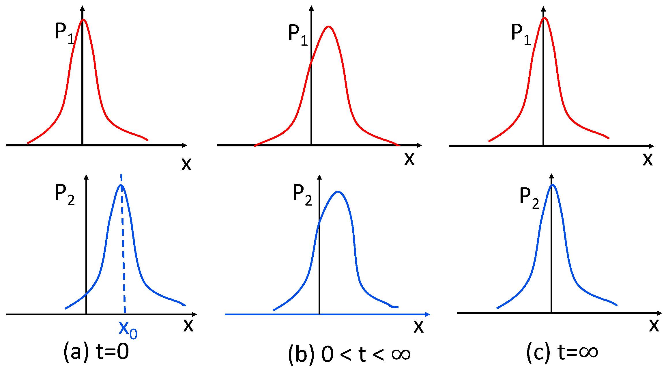

Figure 4.
y and against time for and 3 in (a,c), respectively; the corresponding geodesic circular segments in the upper half-plane in (b,d), respectively. In both cases, and . (Figure 3 in [15]).

Publisher’s Note: MDPI stays neutral with regard to jurisdictional claims in published maps and institutional affiliations. |
© 2021 by the author. Licensee MDPI, Basel, Switzerland. This article is an open access article distributed under the terms and conditions of the Creative Commons Attribution (CC BY) license (https://creativecommons.org/licenses/by/4.0/).
Share and Cite
MDPI and ACS Style
Kim, E.-j. Information Geometry, Fluctuations, Non-Equilibrium Thermodynamics, and Geodesics in Complex Systems. Entropy 2021, 23, 1393. https://0-doi-org.brum.beds.ac.uk/10.3390/e23111393
AMA Style
Kim E-j. Information Geometry, Fluctuations, Non-Equilibrium Thermodynamics, and Geodesics in Complex Systems. Entropy. 2021; 23(11):1393. https://0-doi-org.brum.beds.ac.uk/10.3390/e23111393
Chicago/Turabian StyleKim, Eun-jin. 2021. "Information Geometry, Fluctuations, Non-Equilibrium Thermodynamics, and Geodesics in Complex Systems" Entropy 23, no. 11: 1393. https://0-doi-org.brum.beds.ac.uk/10.3390/e23111393
Note that from the first issue of 2016, this journal uses article numbers instead of page numbers. See further details here.