
Fast Approximations of the Jeffreys Divergence between Univariate Gaussian Mixtures via Mixture Conversions to Exponential-Polynomial Distributions


Sony Computer Science Laboratories, Tokyo 141-0022, Japan
Entropy 2021, 23(11), 1417; https://0-doi-org.brum.beds.ac.uk/10.3390/e23111417
Submission received: 7 September 2021
/
Revised: 20 October 2021
/
Accepted: 26 October 2021
/
Published: 28 October 2021
(This article belongs to the Special Issue Distance in Information and Statistical Physics III)
Abstract
:The Jeffreys divergence is a renown arithmetic symmetrization of the oriented Kullback–Leibler divergence broadly used in information sciences. Since the Jeffreys divergence between Gaussian mixture models is not available in closed-form, various techniques with advantages and disadvantages have been proposed in the literature to either estimate, approximate, or lower and upper bound this divergence. In this paper, we propose a simple yet fast heuristic to approximate the Jeffreys divergence between two univariate Gaussian mixtures with arbitrary number of components. Our heuristic relies on converting the mixtures into pairs of dually parameterized probability densities belonging to an exponential-polynomial family. To measure with a closed-form formula the goodness of fit between a Gaussian mixture and an exponential-polynomial density approximating it, we generalize the Hyvärinen divergence to -Hyvärinen divergences. In particular, the 2-Hyvärinen divergence allows us to perform model selection by choosing the order of the exponential-polynomial densities used to approximate the mixtures. We experimentally demonstrate that our heuristic to approximate the Jeffreys divergence between mixtures improves over the computational time of stochastic Monte Carlo estimations by several orders of magnitude while approximating the Jeffreys divergence reasonably well, especially when the mixtures have a very small number of modes.
1. Introduction
1.1. Statistical Mixtures and Statistical Divergences
We consider the problem of approximating the Jeffreys divergence [1] between two finite univariate continuous mixture models [2] and with continuous component distributions ’s and s defined on a coinciding support . The mixtures and may have a different number of components (i.e., ). Historically, Pearson [3] first considered a univariate Gaussian mixture of two components for modeling the distribution of the ratio of forehead breadth to body length of a thousand crabs in 1894 (Pearson obtained a unimodal mixture).
Although our work applies to any continuous mixtures of an exponential family (e.g., Rayleigh mixtures [4] with restricted support ), we explain our method for the most prominent family of mixtures encountered in practice: the Gaussian mixture models or GMMs for short. In the remainder, a univariate GMM with k Gaussian components
is called a k-GMM.
The KLD is an oriented divergence since .
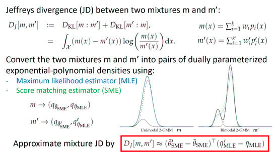
The Jeffreys divergence (JD) [1] is the arithmetic symmetrization of the forward KLD and the reverse KLDs:
The JD is a symmetric divergence: . In the literature, the Jeffreys divergence [7] has also been called the J-divergence [8,9], the symmetric Kullback–Leibler divergence [10] and sometimes the symmetrical Kullback–Leibler divergence [11,12]. In general, it is provably hard to calculate the definite integral of the KLD between two continuous mixtures in closed-form: For example, the KLD between two GMMs has been shown to be non-analytic [13]. Thus, in practice, when calculating the JD between two GMMs, one can either approximate [14,15], estimate [16], or bound [17,18] the KLD between mixtures. Another approach to bypass the computational intractability of calculating the KLD between mixtures consists of designing new types of divergences that admit closed-form expressions for mixtures. See, for example, the Cauchy–Schwarz divergence [19] or the total square divergence [20] (a total Bregman divergence) that admit the closed-form formula when handling GMMs. The total square divergence [20] is invariant to rigid transformations and provably robust to outliers in clustering applications.
In practice, to estimate the KLD between mixtures, one uses the following Monte Carlo (MC) estimator:
where is s independent and identically distributed (i.i.d.) samples from . This MC estimator is by construction always non-negative and therefore consistent. That is, we have under mild conditions [21].
Similarly, we estimate the Jeffreys divergence via MC sampling as follows:
where are s i.i.d. samples from the “middle mixture” . By choosing the middle mixture for sampling, we ensure that we keep the symmetric property of the JD (i.e., ), and we also have consistency under mild conditions [21]: . The time complexity to stochastically estimate the JD is , with s typically ranging from to in applications. Notice that the number of components of a mixture can be very large (e.g., for n input data when using Kernel Density Estimators [2]). KDEs may also have a large number of components and may potentially exhibit many spurious modes visualized as small bumps when plotting the densities.
1.2. Jeffreys Divergence between Densities of an Exponential Family
We consider approximating the JD by converting continuous mixtures into densities of exponential families [22]. A continuous exponential family (EF) of order D is defined as a family of probability density functions with support and the probability density function:
where is called the log-normalizer, which ensures the normalization of (i.e., ):
Parameter is called the natural parameter, and the functions , …, are called the sufficient statistics [22]. Let denote the natural parameter space: , an open convex domain for regular exponential families [22]. The exponential family is said to be minimal when the functions are linearly independent.
It is well-known that one can bypass the definite integral calculation of the KLD when the probability density functions and belong to the same exponential family [23,24]:
where is the Bregman divergence induced by the log-normalizer, a strictly convex real-analytic function [22]. The Bregman divergence [25] between two parameters and for a strictly convex and smooth generator F is defined by:
Thus, the Jeffreys divergence between two pdfs and belonging to the same exponential family is a symmetrized Bregman divergence [26]:
Let denote the Legendre–Fenchel convex conjugate of :
The Legendre transform ensures that and , and the Jeffreys divergence between two pdfs and belonging to the same exponential family is:
Notice that the log-normalizer does not appear explicitly in the above formula.
1.3. A Simple Approximation Heuristic
Densities of an exponential family admit a dual parameterization [22]: , called the moment parameterization (or mean parameterization). Let H denote the moment parameter space. Let us use the subscript and superscript notations to emphasize the coordinate system used to index a density: In our notation, we thus write .
In view of Equation (7), our method to approximate the Jeffreys divergence between mixtures m and consists of first converting those mixtures m and into pairs of polynomial exponential densities (PEDs) in Section 2. To convert a mixture into a pair dually parameterized (but not dual because ), we shall consider “integral extensions” (or information projections) of the Maximum Likelihood Estimator [22] (MLE estimates in the moment parameter space ) and of the Score Matching Estimator [27] (SME estimates in the natural parameter space ).
We shall consider polynomial exponential families [28] (PEFs) also called exponential-polynomial families (EPFs) [29]. PEFs are regular minimal exponential families with polynomial sufficient statistics for . For example, the exponential distributions form a PEF with , and , and the normal distributions form an EPF with , and , etc. Although the log-normalizer can be obtained in closed-form for lower order PEFs (e.g., or ) or very special subfamilies (e.g., when and , exponential-monomial families [30]), a no-closed form formula is available for of EPFs in general as soon [31,32], and the cumulant function is said to be computationally intractable. Notice that when , the leading coefficient is negative for even integer order D. EPFs are attractive because these families can universally model any smooth multimodal distribution [28] and require fewer parameters in comparison to GMMs: Indeed, a univariate k-GMM (at most k modes and antimodes) requires parameters to specify (or for a KDE with constant kernel width or for a KDE with varying kernel widths, but then observations). A density of an EPF of order D is called an exponential-polynomial density (EPD) and requires D parameters to specify , with, at most, modes (and antimodes). The case of the quartic (polynomial) exponential densities () has been extensively investigated in [31,33,34,35,36,37]. Armstrong and Brigo [38] discussed order-6 PEDs, and Efron and Hastie reported and order-7 PEF in their textbook (see Figure 5.7 of [39]). Figure 1 displays two examples of converting a GMM into a pair of dually parameterized exponential-polynomial densities.
Then by converting both mixture m and mixture into pairs of dually natural/moment parameterized unnormalized PEDs, i.e., and , we approximate the JD between mixtures m and by using the four parameters of the PEDs
Let denote the approximation formula obtained from the two pairs of PEDs:
Let . Then we have
Note that is not a proper divergence as it may be negative since, in general, . That is, may not satisfy the law of the indiscernibles. Approximation is exact when , with both m and belonging to an exponential family.
We experimentally show in Section 4 that the heuristic yields fast approximations of the JD compared to the MC baseline estimations by several order of magnitudes while approximating the JD reasonably well when the mixtures have a small number of modes.
For example, Figure 2 displays the unnormalized PEDs obtained for two Gaussian mixture models ( components and components) into PEDs of a PEF of order . The MC estimation of the JD with samples yields , while the PED approximation of Equation (8) on corresponding PEFs yields (the relative error is or about ). It took about milliseconds (with on a Dell Inspiron 7472 laptop) to MC estimate the JD, while it took about milliseconds with the PEF approximation. Thus, we obtained a speed-up factor of about 3190 (three orders of magnitude) for this particular example. Notice that when viewing Figure 2, we tend to visually evaluate the dissimilarity using the total variation distance (a metric distance):
rather than by a dissimilarity relating to the KLD. Using Pinsker’s inequality [40,41], we have and . Thus, large TV distance (e.g., ) between mixtures may have a small JD since Pinsker’s inequality yields .
Let us point out that our approximation heuristic is deterministic, while the MC estimations are stochastic: That is, each MC run (Equation (4)) returns a different result, and a single MC run may yield a very bad approximation of the true Jeffreys divergence.
We compare our fast heuristic with two more costly methods relying on numerical procedures to convert natural ↔ moment parameters:
- Simplify GMMs into , and approximately convert the ’s into ’s. Then approximate the Jeffreys divergence as
- Simplify GMMs into , and approximately convert the ’s into ’s. Then approximate the Jeffreys divergence as
1.4. Contributions and Paper Outline
Our contributions are summarized as follows:
- We explain how to convert any continuous density (including GMMs) into a polynomial exponential density in Section 2 using integral-based extensions of the Maximum Likelihood Estimator [22] (MLE estimates in the moment parameter space H, Theorem 1 and Corollary 1) and the Score Matching Estimator [27] (SME estimates in the natural parameter space , Theorem 3). We show a connection between SME and the Moment Linear System Estimator [28] (MLSE).
- We show how to approximate the Jeffreys divergence between GMMs using a pair of natural/moment parameter PED conversion and present experimental results that display a gain of several orders of magnitude of performance when compared to the vanilla Monte Carlo estimator in Section 4. We observe that the quality of the approximations depend on the number of modes of the GMMs [43]. However, calculating or counting the modes of a GMM is a difficult problem in its own [43].
The paper is organized as follows: In Section 2, we show how to convert arbitrary probability density functions into polynomial exponential densities using the integral-based Maximum Likelihood Estimator (MLE) and Score Matching Estimator (SME). We describe a Maximum Entropy method to iteratively convert moment parameters into natural parameters in Section 2.3.1. It is followed by Section 3, which shows how to calculate in closed-form the order-2 Hyvärinen divergence between a GMM and a polynomial exponential density. We use this criterion to perform model selection. Section 4 presents our computational experiments that demonstrate a gain of several orders of magnitudes for GMMs with a small number of modes. Finally, we conclude in Section 5.
2. Converting Finite Mixtures to Exponential Family Densities
We report two generic methods to convert a mixture into a density of an exponential family: The first method extending the MLE in Section 2.1 proceeds using the mean parameterization , while the second method extending the SME in Section 2.2 uses the natural parameterization of the exponential family. We then describe how to convert the moments parameters into natural parameters (and vice versa) for polynomial exponential families in Section 2.3. We show how to instantiate these generic conversion methods for GMMs: It requires calculating non-central moments of GMMs in closed-form. The efficient computations of raw moments of GMMs is detailed in Section 2.4.
2.1. Conversion Using the Moment Parameterization (MLE)
Let us recall that in order to estimate the moment or mean parameter of a density belonging an exponential family
with a sufficient statistic vector from an i.i.d. sample set , the Maximum Likelihood Estimator (MLE) [22,44] yields
In statistics, Equation (12) is called the estimating equation. The MLE exists under mild conditions [22] and is unique since the Hessian of the estimating equation is positive-definite (log-normalizers are always strictly convex and real analytic [22]). The MLE is consistent and asymptotically normally distributed [22]. Furthermore, since the MLE satisfies the equivariance property [22], we have , where denotes the gradient of the conjugate function of the cumulant function of the exponential family. In general, is intractable for PEDs with .
By considering the empirical distribution
where denotes the Dirac distribution at location , we can formulate the MLE problem as a minimum KLD problem between the empirical distribution and a density of the exponential family:
since the entropy term is independent of .
Thus, to convert an arbitrary smooth density into a density of an exponential family , we have to solve the following minimization problem:
Rewriting the minimization problem as:
we obtain
The minimum is unique since (positive-definite matrix). This conversion procedure can be interpreted as an integral extension of the MLE, hence the notation in . Notice that the ordinary MLE is obtained for the empirical distribution: : .
Theorem 1.
The best density of an exponential family minimizing the Kullback–Leibler divergence between a density r and a density of an exponential family is .
Notice that when , we obtain so that the method is consistent (by analogy to the finite i.i.d. MLE case): .
The KLD right-sided minimization problem can be interpreted as an information projection of r onto . As a corollary of Theorem 1, we obtain:
Corollary 1
(Best right-sided KLD simplification of a mixture). The best right-sided KLD simplification of a homogeneous mixture of exponential families [2] with , i.e., , into a single component is given by .
Equation (16) allows us to greatly simplify the proofs reported in [45] for mixture simplifications that involved the explicit use of the Pythagoras’ theorem in the dually flat spaces of exponential families [42]. Figure 3 displays the geometric interpretation of the best KLD simplification of a GMM with ambient space the probability space , where denotes the Lebesgue measure and the Borel -algebra of .
Let us notice that Theorem 1 yields an algebraic system for polynomial exponential densities, i.e., for , to compute for a given GMM (since raw moments are algebraic). In contrast with this result, the MLE of i.i.d. observations is in general not an algebraic function [46] but a transcendental function.
2.2. Converting to a PEF Using the Natural Parameterization (SME)
Integral-Based Score Matching Estimator (SME)
To convert the density into an exponential density with sufficient statistics , we can also use the Score Matching Estimator [27,47] (SME). The Score Matching Estimator minimizes the Hyvärinen divergence (Equation (4) of [47]):
The Hyvärinen divergence is also known as half of the relative Fisher information in the optimal transport community (Equation (8) of [48] or Equation (2.2) in [49]), where it is defined for two measures and as follows:
Moreover, the relative Fisher information can be defined on complete Riemannian manifolds [48].
That is, we convert a density into an exponential family density using the following minimizing problem:
Beware that in statistics, the score is defined by , but in Score Matching, we refer to the “data score” defined by . Hyvärinen [47] gave an explanation of the naming “score” using a spurious location parameter.
- Generic solution: It can be shown that for exponential families [47], we obtain the following solution:whereis a symmetric matrix, andis a D-dimensional column vector.
Theorem 2.
The best conversion of a density into a density of an exponential family minimizing the right-sided Hyvärinen divergence is
- Solution instantiated for polynomial exponential families:For polynomial exponential families of order D, we have and , and therefore, we haveandwhere denotes the l-th raw moment of distribution (with the convention that ). For a probability density function , we have .Thus, the integral-based SME of a density r is:For example, matrix is
- Faster PEF solutions using Hankel matrices:The method of Cobb et al. [28] (1983) anticipated the Score Matching method of Hyvärinen (2005). It can be derived from Stein’s lemma for exponential families [50]. The integral-based Score Matching method is consistent, i.e., if , then : The probabilistic proof for is reported as Theorem 2 of [28]. The integral-based proof is based on the property that arbitrary order partial mixed derivatives can be obtained from higher-order partial derivatives with respect to [29]:where .The complexity of the direct SME method is as it requires the inverse of the -dimensional matrix .We show how to lower this complexity by reporting an equivalent method (originally presented in [28]) that relies on recurrence relationships between the moments of for PEDs. Recall that denotes the l-th raw moment .Let denote the symmetric matrix with (with ), and the D-dimensional vector with . We solve the system to obtain . We then obtain the natural parameter from the vector asNow, if we inspect matrix , we find that matrix is a Hankel matrix: A Hankel matrix has constant anti-diagonals and can be inverted in quadratic-time [51,52] instead of cubic time for a general matrix. (The inverse of a Hankel matrix is a Bezoutian matrix [53].) Moreover, a Hankel matrix can be stored using linear memory (store coefficients) instead of quadratic memory of regular matrices.For example, matrix is:and requires only coefficients to be stored instead of . The order-d moment matrix isis a Hankel matrix stored using coefficients:In statistics, those matrices are called moment matrices and well-studied [54,55,56]. The variance of a random variable X can be expressed as the determinant of the order-2 moment matrix:This observation yields a generalization of the notion of variance to random variables: . The variance can be expressed as for . See [57] (Chapter 5) for a detailed description related to U-statistics.For GMMs r, the raw moments to build matrix can be calculated in closed-form, as explained in Section 2.4.
Theorem 3 (Score matching GMM conversion)
The Score Matching conversion of a GMM into a polynomial exponential density of order D is obtained as
where denote the ith non-central moment of the GMM .
2.3. Converting Numerically Moment Parameters from/to Natural Parameters
Recall that our fast heuristic approximates the Jeffreys divergence by
Because F and are not available in closed form (except for the case of the normal family), we cannot obtain from a given (using ) nor from a given (using ).
However, provided that we can approximate numerically and , we also consider these two approximations for the Jeffreys divergence:
and
We show how to numerically estimate from in Section 2.3.1. Next, in Section 2.3.2, we show how to stochastically estimate .
2.3.1. Converting Moment Parameters to Natural Parameters Using Maximum Entropy
Let us report the iterative approximation technique of [58] (which extended the method described in [35]) based on solving a maximum entropy problem (MaxEnt problem). This method will be useful when comparing our fast heuristic with the approximations and .
The density of any exponential family can be characterized as a maximum entropy distribution given the D moment constraints : Namely, subject to the moment constraints for , where we added by convention and (so that ). The solution of this MaxEnt problem [58] is , where are the Lagrangian parameters. Here, we adopt the following canonical parameterization of the densities of an exponential family:
That is, and for . Parameter is a kind of augmented natural parameter that includes the log-normalizer in its first coefficient.
Let denote the set of non-linear equations for . The Iterative Linear System Method [58] (ILSM) converts to iteratively. We initialize to (and calculate numerically ).
At iteration t with current estimate , we use the following first-order Taylor approximation:
Let denote the matrix:
We have
We update as follows:
For a PEF of order D, we have
This yields a moment matrix (Hankel matrix), which can be inverted in quadratic time [52]. In our setting, the moment matrix is invertible because , see [59].
Let denote after T iterations (retrieved from ) and the corresponding natural parameter of the PED. We have the following approximation of the JD:
The method is costly because we need to numerically calculate and the ’s (e.g., univariate Simpson integrator). Another potential method consists of estimating these expectations using acceptance-rejection sampling [60,61]. We may also consider the holonomic gradient descent [29]. Thus, the conversion method is costly. Our heuristic bypasses this costly moment-to-natural parameter conversion by converting each mixture m to a pair of PEDs parameterized in the natural and moment parameters (i.e., loosely speaking, we untangle these dual parameterizations).
2.3.2. Converting Natural Parameters to Moment Parameters
2.4. Raw Non-Central Moments of Normal Distributions and GMMs
In order to implement the MLE or SME Gaussian mixture conversion procedures, we need to calculate the raw moments of a Gaussian mixture model. The l-th moment raw moment of a standard normal distribution is 0 when l is odd (since the normal standard density is an even function) and when l is even, where is the double factorial (with by convention). Using the binomial theorem, we deduce that a normal distribution has finite moments:
That is, we have
where denotes the double factorial:
By the linearity of the expectation , we deduce the l-th raw moment of a GMM :
3. Goodness-of-Fit between GMMs and PEDs: Higher Order Hyvärinen Divergences
Once we have converted a GMM into an unnormalized PED , we would like to evaluate the quality of the conversion, i.e., , using a statistical divergence . This divergence shall allow us to perform model selection by choosing the order D of the PEF so that for , where is a prescribed threshold. Since PEDs have computationally intractable normalization constants, we consider a right-sided projective divergence [42] that satisfies for any . For example, we may consider the -divergence [65] that is a two-sided projective divergence: for any and converge to the KLD when . However, the -divergence between a mixture model and an unnormalized PEF does not yield a closed-form formula. Moreover, the -divergence between two unnormalized PEDs is expressed using the log-normalizer function that is computationally intractable [66].
In order to a get a closed-form formula for a divergence between a mixture model and an unnormalized PED, we consider the order- (for ) Hyvärinen divergence [42] as follows:
The Hyvärinen divergence [42] (order-1 Hyvärinen divergence) has also been called the Fisher divergence [27,67,68,69] or relative Fisher information [48]. Notice that when , , the ordinary Hyvärinen divergence [27].
The Hyvärinen divergences is a right-sided projective divergence, meaning that the divergence satisfies for any . That is, we have . Thus, we have for an unnormalized PED . For statistical estimation, it is enough to have a sided projective divergence since we need to evaluate the goodness of fit between the (normalized) empirical distribution and the (unnormalized) parameteric density.
For univariate distributions, , and , where is the unnormalized model.
Let be a homogeneous polynomial defining the shape of the EPF:
For PEDs with the homogeneous polynomial , we have .
Theorem 4.
The Hyvärinen divergence of order 2 between a Gaussian mixture and a polynomial exponential family density is available in closed form.
Proof.
We have with
denoting the derivative of the Gaussian mixture density . It follows that:
where
Therefore, we have
with .
Therefore, we obtain
Thus, the Hyvärinen divergence of order 2 between a GMM and a PED is available in closed-form. □
For example, when (i.e., mixture m is a single Gaussian ) and is a normal distribution (i.e., PED with , ), we obtain the following formula for the order-2 Hyvärinen divergence:
4. Experiments: Jeffreys Divergence between Mixtures
In this section, we evaluate our heuristic to approximate the Jeffreys divergence between two mixtures m and :
Recall that stochastically estimating the JD between k-GMMs with Monte Carlo sampling using s samples (i.e., ) requires and is not deterministic. That is, different MC runs yield fluctuating values that may be fairly different. In comparison, approximating by using by converting mixtures to D-order PEDs require time to compute the raw moments and time to invert a Hankel moment matrix. Thus, by choosing , we obtain a deterministic algorithm that is faster than the MC sampling when . Since there are, at most, k modes for a k-GMM, we choose order for the PEDs.
To obtain quantitative results on the performance of our heuristic , we build random GMMs with k components as follows: , where , and , where the ’s, and and are independent uniform distributions on . The mixture weights are then normalized to sum up to one. For each value of k, we make 1000 trial experiments to gather statistics and use for evaluating the Jeffreys divergence by Monte Carlo samplings. We denote by the error of an experiment. Table 1 presents the results of the experiments for : The table displays the average error, the maximum error (minimum error is very close to zero, of order ), and the speed-up obtained by our heuristic . Those experiments were carried out on a Dell Inspiron 7472 laptop (equipped with an Intel(R) Core(TM) i5-8250U CPU at 1.60 GHz).
Notice that the quality of the approximations of depend on the number of modes of the GMMs. However, calculating the number of modes is difficult [43,70], even for simple cases [71,72].
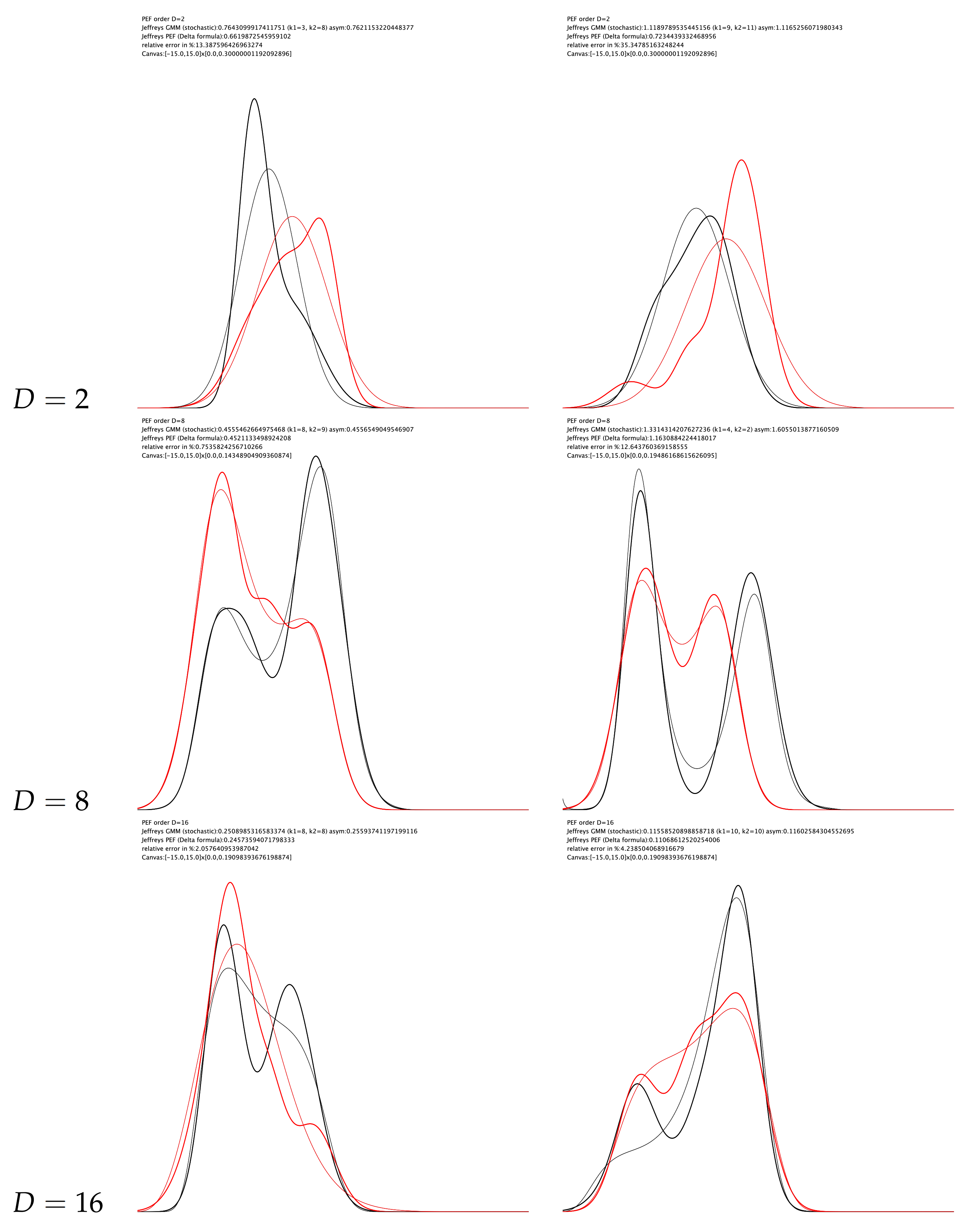
Figure 4 displays several experiments of converting mixtures to pairs of PEDs to obtain approximations of the Jeffreys divergence.
Figure 5 illustrates the use of the order-2 Hyvärinen divergence to perform model selection for choosing the order of a PED.
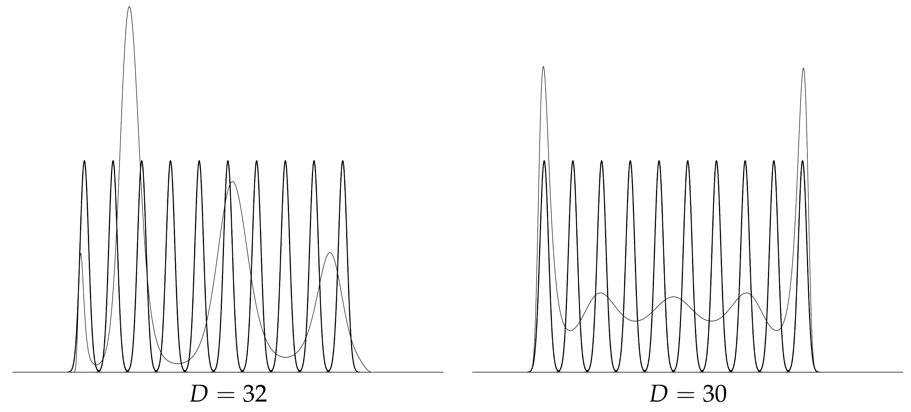
Finally, Figure 6 displays some limitations of the GMM to PED conversion when the GMMs have many modes. In that case, running the conversion to obtain and estimate the Jeffreys divergence by
improves the results but requires more computation.
Next, we consider learning a PED by converting a GMM derived itself from a Kernel Density Estimator (KDE). We use the duration of the eruption for the Old Faithful geyser in Yellowstone National Park (Wyoming, USA): The dataset consists of 272 observations (https://www.stat.cmu.edu/~larry/all-of-statistics/=data/faithful.dat) (access date: 25 October 2021) and is included in the R language package ‘stats’. Figure 7 displays the GMMs obtained from the KDEs of the Old Faithful geyser dataset when choosing for each component (left) and . Observe that the data are bimodal once the spurious modes (i.e., small bumps) are removed, as studied in [32]. Barron and Sheu [32] modeled that dataset using a bimodal PED of order , i.e., a quartic distribution. We model it with a PED of order using the integral-based Score Matching method. Figure 8 displays the unnormalized bimodal density (i.e., ) that we obtained using the integral-based Score Matching method (with ).
5. Conclusions and Perspectives
Many applications [7,73,74,75] require computing the Jeffreys divergence (the arithmetic symmetrization of the Kullback–Leibler divergence) between Gaussian mixture models. Since the Jeffreys divergence between GMMs is provably not available in closed-form [13], one often ends up implementing a costly Monte Carlo stochastic approximation of the Jeffreys divergence. In this paper, we first noticed the simple expression of the Jeffreys divergence between densities and of an exponential family using their dual natural and moment parameterizations [22] and :
where and for the cumulant function of the exponential family. This led us to propose a simple and fast heuristic to approximate the Jeffreys divergence between Gaussian mixture models: First, convert a mixture m to a pair of dually parameterized polynomial exponential densities using extensions of the Maximum Likelihood and Score Matching Estimators (Theorems 1 and 3), and then approximate the JD deterministically by
The order of the polynomial exponential family may be either prescribed or selected using the order-2 Hyvärinen divergence, which evaluates in closed form the dissimilarity between a GMM and a density of an exponential-polynomial family (Theorem 4). We experimentally demonstrated that the Jeffreys divergence between GMMs can be reasonably well approximated by for mixtures with a small number of modes, and we obtained an overall speed-up of several order of magnitudes compared to the Monte Carlo sampling method. We also propose another deterministic heuristic to estimate as
where is numerically calculated using an iterative conversion procedure based on maximum entropy [58] (Section 2.3.1). Our technique extends to other univariate mixtures of exponential families (e.g., mixtures of Rayleigh distributions, mixtures of Gamma distributions, or mixtures of Beta distributions, etc). One limitation of our method is that the PED modeling of a GMM may not guarantee obtaining the same number of modes as the GMM even when we increase the order D of the exponential-polynomial densities. This case is illustrated in Figure 9 (right).
Although PEDs are well-suited to calculate Jeffreys divergence compared to GMMs, we point out that GMMs are better suited for sampling, while PEDs require Monte Carlo methods (e.g., adaptive rejection sampling or MCMC methods [62]). Furthermore, we can estimate the Kullback–Leibler divergence between two PEDs using rejection sampling (or other McMC methods [62]) or by using the -divergence [76] with close to zero [66] (e.g., ). The web page of the project is https://franknielsen.github.io/JeffreysDivergenceGMMPEF/index.html (accessed on 25 October 2021).
Funding
This research received no external funding.
Informed Consent Statement
Not applicable.
Data Availability Statement
Not applicable.
Conflicts of Interest
The authors declare no conflict of interest.
References
- Jeffreys, H. An invariant form for the prior probability in estimation problems. Proc. R. Soc. Lond. Ser. A Math. Phys. Sci. 1946, 186, 453–461. [Google Scholar]
- McLachlan, G.J.; Basford, K.E. Mixture Models: Inference and Applications to Clustering; M. Dekker: New York, NY, USA, 1988; Volume 38. [Google Scholar]
- Pearson, K. Contributions to the mathematical theory of evolution. Philos. Trans. R. Soc. Lond. A 1894, 185, 71–110. [Google Scholar]
- Seabra, J.C.; Ciompi, F.; Pujol, O.; Mauri, J.; Radeva, P.; Sanches, J. Rayleigh mixture model for plaque characterization in intravascular ultrasound. IEEE Trans. Biomed. Eng. 2011, 58, 1314–1324. [Google Scholar] [CrossRef] [PubMed]
- Kullback, S. Information Theory and Statistics; Courier Corporation: North Chelmsford, MA, USA, 1997. [Google Scholar]
- Cover, T.M. Elements of Information Theory; John Wiley & Sons: Hoboken, NJ, USA, 1999. [Google Scholar]
- Vitoratou, S.; Ntzoufras, I. Thermodynamic Bayesian model comparison. Stat. Comput. 2017, 27, 1165–1180. [Google Scholar] [CrossRef] [Green Version]
- Kannappan, P.; Rathie, P. An axiomatic characterization of J-divergence. In Transactions of the Tenth Prague Conference on Information Theory, Statistical Decision Functions, Random Processes; Springer: Dordrecht, The Netherlands, 1988; pp. 29–36. [Google Scholar]
- Burbea, J. J-Divergences and related concepts. Encycl. Stat. Sci. 2004. [Google Scholar] [CrossRef]
- Tabibian, S.; Akbari, A.; Nasersharif, B. Speech enhancement using a wavelet thresholding method based on symmetric Kullback–Leibler divergence. Signal Process. 2015, 106, 184–197. [Google Scholar] [CrossRef]
- Veldhuis, R. The centroid of the symmetrical Kullback-Leibler distance. IEEE Signal Process. Lett. 2002, 9, 96–99. [Google Scholar] [CrossRef] [Green Version]
- Nielsen, F. Jeffreys centroids: A closed-form expression for positive histograms and a guaranteed tight approximation for frequency histograms. IEEE Signal Process. Lett. 2013, 20, 657–660. [Google Scholar] [CrossRef] [Green Version]
- Watanabe, S.; Yamazaki, K.; Aoyagi, M. Kullback information of normal mixture is not an analytic function. IEICE Tech. Rep. Neurocomput. 2004, 104, 41–46. [Google Scholar]
- Cui, S.; Datcu, M. Comparison of Kullback-Leibler divergence approximation methods between Gaussian mixture models for satellite image retrieval. In Proceedings of the 2015 IEEE International Geoscience and Remote Sensing Symposium (IGARSS), Milan, Italy, 26–31 July 2015; pp. 3719–3722. [Google Scholar]
- Cui, S. Comparison of approximation methods to Kullback–Leibler divergence between Gaussian mixture models for satellite image retrieval. Remote Sens. Lett. 2016, 7, 651–660. [Google Scholar] [CrossRef] [Green Version]
- Sreekumar, S.; Zhang, Z.; Goldfeld, Z. Non-asymptotic Performance Guarantees for Neural Estimation of f-Divergences. In Proceedings of the International Conference on Artificial Intelligence and Statistics (PMLR 2021), San Diego, CA, USA, 18–24 July 2021; pp. 3322–3330. [Google Scholar]
- Durrieu, J.L.; Thiran, J.P.; Kelly, F. Lower and upper bounds for approximation of the Kullback-Leibler divergence between Gaussian mixture models. In Proceedings of the 2012 IEEE International Conference on Acoustics, Speech and Signal Processing (ICASSP), Kyoto, Japan, 25–30 March 2012; pp. 4833–4836. [Google Scholar]
- Nielsen, F.; Sun, K. Guaranteed bounds on information-theoretic measures of univariate mixtures using piecewise log-sum-exp inequalities. Entropy 2016, 18, 442. [Google Scholar] [CrossRef] [Green Version]
- Jenssen, R.; Principe, J.C.; Erdogmus, D.; Eltoft, T. The Cauchy–Schwarz divergence and Parzen windowing: Connections to graph theory and Mercer kernels. J. Frankl. Inst. 2006, 343, 614–629. [Google Scholar] [CrossRef]
- Liu, M.; Vemuri, B.C.; Amari, S.i.; Nielsen, F. Shape retrieval using hierarchical total Bregman soft clustering. IEEE Trans. Pattern Anal. Mach. Intell. 2012, 34, 2407–2419. [Google Scholar]
- Robert, C.; Casella, G. Monte Carlo Statistical Methods; Springer Science & Business Media: Berlin/Heidelberg, Germany, 2013. [Google Scholar]
- Barndorff-Nielsen, O. Information and Exponential Families: In Statistical Theory; John Wiley & Sons: Hoboken, NJ, USA, 2014. [Google Scholar]
- Azoury, K.S.; Warmuth, M.K. Relative loss bounds for on-line density estimation with the exponential family of distributions. Mach. Learn. 2001, 43, 211–246. [Google Scholar] [CrossRef] [Green Version]
- Banerjee, A.; Merugu, S.; Dhillon, I.S.; Ghosh, J. Clustering with Bregman divergences. J. Mach. Learn. Res. 2005, 6, 1705–1749. [Google Scholar]
- Bregman, L.M. The relaxation method of finding the common point of convex sets and its application to the solution of problems in convex programming. USSR Comput. Math. Math. Phys. 1967, 7, 200–217. [Google Scholar] [CrossRef]
- Nielsen, F.; Nock, R. Sided and symmetrized Bregman centroids. IEEE Trans. Inf. Theory 2009, 55, 2882–2904. [Google Scholar] [CrossRef] [Green Version]
- Hyvärinen, A. Estimation of non-normalized statistical models by score matching. J. Mach. Learn. Res. 2005, 6, 695–709. [Google Scholar]
- Cobb, L.; Koppstein, P.; Chen, N.H. Estimation and moment recursion relations for multimodal distributions of the exponential family. J. Am. Stat. Assoc. 1983, 78, 124–130. [Google Scholar] [CrossRef]
- Hayakawa, J.; Takemura, A. Estimation of exponential-polynomial distribution by holonomic gradient descent. Commun. Stat.-Theory Methods 2016, 45, 6860–6882. [Google Scholar] [CrossRef] [Green Version]
- Nielsen, F.; Nock, R. MaxEnt upper bounds for the differential entropy of univariate continuous distributions. IEEE Signal Process. Lett. 2017, 24, 402–406. [Google Scholar] [CrossRef]
- Matz, A.W. Maximum likelihood parameter estimation for the quartic exponential distribution. Technometrics 1978, 20, 475–484. [Google Scholar] [CrossRef]
- Barron, A.R.; Sheu, C.H. Approximation of density functions by sequences of exponential families. Ann. Stat. 1991, 19, 1347–1369, Correction in 1991, 19, 2284–2284. [Google Scholar]
- O’toole, A. A method of determining the constants in the bimodal fourth degree exponential function. Ann. Math. Stat. 1933, 4, 79–93. [Google Scholar] [CrossRef]
- Aroian, L.A. The fourth degree exponential distribution function. Ann. Math. Stat. 1948, 19, 589–592. [Google Scholar] [CrossRef]
- Zellner, A.; Highfield, R.A. Calculation of maximum entropy distributions and approximation of marginal posterior distributions. J. Econom. 1988, 37, 195–209. [Google Scholar] [CrossRef]
- McCullagh, P. Exponential mixtures and quadratic exponential families. Biometrika 1994, 81, 721–729. [Google Scholar] [CrossRef]
- Mead, L.R.; Papanicolaou, N. Maximum entropy in the problem of moments. J. Math. Phys. 1984, 25, 2404–2417. [Google Scholar] [CrossRef] [Green Version]
- Armstrong, J.; Brigo, D. Stochastic filtering via L2 projection on mixture manifolds with computer algorithms and numerical examples. arXiv 2013, arXiv:1303.6236. [Google Scholar]
- Efron, B.; Hastie, T. Computer Age Statistical Inference; Cambridge University Press: Cambridge, UK, 2016; Volume 5. [Google Scholar]
- Pinsker, M. Information and Information Stability of Random Variables and Processes (Translated and Annotated by Amiel Feinstein); Holden-Day Inc.: San Francisco, CA, USA, 1964. [Google Scholar]
- Fedotov, A.A.; Harremoës, P.; Topsoe, F. Refinements of Pinsker’s inequality. IEEE Trans. Inf. Theory 2003, 49, 1491–1498. [Google Scholar] [CrossRef]
- Amari, S. Information Geometry and Its Applications; Applied Mathematical Sciences; Springer: Berlin/Heidelberg, Germany, 2016. [Google Scholar]
- Carreira-Perpinan, M.A. Mode-finding for mixtures of Gaussian distributions. IEEE Trans. Pattern Anal. Mach. Intell. 2000, 22, 1318–1323. [Google Scholar] [CrossRef] [Green Version]
- Brown, L.D. Fundamentals of statistical exponential families with applications in statistical decision theory. Lect. Notes-Monogr. Ser. 1986, 9, 1–279. [Google Scholar]
- Pelletier, B. Informative barycentres in statistics. Ann. Inst. Stat. Math. 2005, 57, 767–780. [Google Scholar] [CrossRef]
- Améndola, C.; Drton, M.; Sturmfels, B. Maximum likelihood estimates for Gaussian mixtures are transcendental. In Proceedings of the International Conference on Mathematical Aspects of Computer and Information Sciences, Berlin, Germany, 11–13 November 2015; pp. 579–590. [Google Scholar]
- Hyvärinen, A. Some extensions of score matching. Comput. Stat. Data Anal. 2007, 51, 2499–2512. [Google Scholar] [CrossRef] [Green Version]
- Otto, F.; Villani, C. Generalization of an inequality by Talagrand and links with the logarithmic Sobolev inequality. J. Funct. Anal. 2000, 173, 361–400. [Google Scholar] [CrossRef] [Green Version]
- Toscani, G. Entropy production and the rate of convergence to equilibrium for the Fokker-Planck equation. Q. Appl. Math. 1999, 57, 521–541. [Google Scholar] [CrossRef] [Green Version]
- Hudson, H.M. A natural identity for exponential families with applications in multiparameter estimation. Ann. Stat. 1978, 6, 473–484. [Google Scholar] [CrossRef]
- Trench, W.F. An algorithm for the inversion of finite Hankel matrices. J. Soc. Ind. Appl. Math. 1965, 13, 1102–1107. [Google Scholar] [CrossRef]
- Heinig, G.; Rost, K. Fast algorithms for Toeplitz and Hankel matrices. Linear Algebra Its Appl. 2011, 435, 1–59. [Google Scholar] [CrossRef] [Green Version]
- Fuhrmann, P.A. Remarks on the inversion of Hankel matrices. Linear Algebra Its Appl. 1986, 81, 89–104. [Google Scholar] [CrossRef] [Green Version]
- Lindsay, B.G. On the determinants of moment matrices. Ann. Stat. 1989, 17, 711–721. [Google Scholar] [CrossRef]
- Lindsay, B.G. Moment matrices: Applications in mixtures. Ann. Stat. 1989, 17, 722–740. [Google Scholar] [CrossRef]
- Provost, S.B.; Ha, H.T. On the inversion of certain moment matrices. Linear Algebra Its Appl. 2009, 430, 2650–2658. [Google Scholar] [CrossRef]
- Serfling, R.J. Approximation Theorems of Mathematical Statistics; John Wiley & Sons: Hoboken, NJ, USA, 2009; Volume 162. [Google Scholar]
- Mohammad-Djafari, A. A. A Matlab program to calculate the maximum entropy distributions. In Maximum Entropy and Bayesian Methods; Springer: Berlin/Heidelberg, Germany, 1992; pp. 221–233. [Google Scholar]
- Karlin, S. Total Positivity; Stanford University Press: Redwood City, CA, USA, 1968; Volume 1. [Google Scholar]
- von Neumann, J. Various Techniques Used in Connection with Random Digits. In Monte Carlo Method; National Bureau of Standards Applied Mathematics Series; Householder, A.S., Forsythe, G.E., Germond, H.H., Eds.; US Government Printing Office: Washington, DC, USA, 1951; Volume 12, Chapter 13; pp. 36–38. [Google Scholar]
- Flury, B.D. Acceptance-rejection sampling made easy. SIAM Rev. 1990, 32, 474–476. [Google Scholar] [CrossRef]
- Rohde, D.; Corcoran, J. MCMC methods for univariate exponential family models with intractable normalization constants. In Proceedings of the 2014 IEEE Workshop on Statistical Signal Processing (SSP), Gold Coast, Australia, 29 June–2 July 2014; pp. 356–359. [Google Scholar]
- Barr, D.R.; Sherrill, E.T. Mean and variance of truncated normal distributions. Am. Stat. 1999, 53, 357–361. [Google Scholar]
- Amendola, C.; Faugere, J.C.; Sturmfels, B. Moment Varieties of Gaussian Mixtures. J. Algebr. Stat. 2016, 7, 14–28. [Google Scholar] [CrossRef] [Green Version]
- Fujisawa, H.; Eguchi, S. Robust parameter estimation with a small bias against heavy contamination. J. Multivar. Anal. 2008, 99, 2053–2081. [Google Scholar] [CrossRef] [Green Version]
- Nielsen, F.; Nock, R. Patch matching with polynomial exponential families and projective divergences. In Proceedings of the International Conference on Similarity Search and Applications, Tokyo, Japan, 24–26 October 2016; pp. 109–116. [Google Scholar]
- Yang, Y.; Martin, R.; Bondell, H. Variational approximations using Fisher divergence. arXiv 2019, arXiv:1905.05284. [Google Scholar]
- Kostrikov, I.; Fergus, R.; Tompson, J.; Nachum, O. Offline reinforcement learning with Fisher divergence critic regularization. In Proceedings of the International Conference on Machine Learning (PMLR 2021), online, 7–8 June 2021; pp. 5774–5783. [Google Scholar]
- Elkhalil, K.; Hasan, A.; Ding, J.; Farsiu, S.; Tarokh, V. Fisher Auto-Encoders. In Proceedings of the International Conference on Artificial Intelligence and Statistics (PMLR 2021), San Diego, CA, USA, 13–15 April 2021; pp. 352–360. [Google Scholar]
- Améndola, C.; Engström, A.; Haase, C. Maximum number of modes of Gaussian mixtures. Inf. Inference J. IMA 2020, 9, 587–600. [Google Scholar] [CrossRef]
- Aprausheva, N.; Mollaverdi, N.; Sorokin, S. Bounds for the number of modes of the simplest Gaussian mixture. Pattern Recognit. Image Anal. 2006, 16, 677–681. [Google Scholar] [CrossRef] [Green Version]
- Aprausheva, N.; Sorokin, S. Exact equation of the boundary of unimodal and bimodal domains of a two-component Gaussian mixture. Pattern Recognit. Image Anal. 2013, 23, 341–347. [Google Scholar] [CrossRef]
- Xiao, Y.; Shah, M.; Francis, S.; Arnold, D.L.; Arbel, T.; Collins, D.L. Optimal Gaussian mixture models of tissue intensities in brain MRI of patients with multiple-sclerosis. In Proceedings of the International Workshop on Machine Learning in Medical Imaging, Beijing, China, 20 September 2010; pp. 165–173. [Google Scholar]
- Bilik, I.; Khomchuk, P. Minimum divergence approaches for robust classification of ground moving targets. IEEE Trans. Aerosp. Electron. Syst. 2012, 48, 581–603. [Google Scholar] [CrossRef]
- Alippi, C.; Boracchi, G.; Carrera, D.; Roveri, M. Change Detection in Multivariate Datastreams: Likelihood and Detectability Loss. In Proceedings of the Twenty-Fifth International Joint Conference on Artificial Intelligence, IJCAI 2016, New York, NY, USA, 9–15 July 2016. [Google Scholar]
- Eguchi, S.; Komori, O.; Kato, S. Projective power entropy and maximum Tsallis entropy distributions. Entropy 2011, 13, 1746–1764. [Google Scholar] [CrossRef]
- Orjebin, E. A Recursive Formula for the Moments of a Truncated Univariate Normal Distribution. 2014, Unpublished note.
- Del Castillo, J. The singly truncated normal distribution: A non-steep exponential family. Ann. Inst. Stat. Math. 1994, 46, 57–66. [Google Scholar] [CrossRef] [Green Version]
Figure 1.
Two examples illustrating the conversion of a GMM m (black) of components (dashed black) into a pair of polynomial exponential densities of order . PED is displayed in green, and PED is displayed in blue. To display , we first converted to using an iterative linear system descent method (ILSDM), and we numerically estimated the normalizing factors and to display the normalized PEDs.

Figure 2.
Two mixtures (black) and (red) of components and components (left), respectively. The unnormalized PEFs (middle) and (right) of order . Jeffreys divergence (about ) is approximated using PEDs within compared to the Monte Carlo estimate with a speed factor of about 3190. Notice that displaying and on the same PDF canvas as the mixtures would require calculating the partition functions and (which we do not in this figure). The PEDs and of the pairs and parameterized in the moment space are not shown here.

Figure 3.
The best simplification of a GMM into a single normal component () is geometrically interpreted as the unique m-projection of onto the Gaussian family (a e-flat): We have .
Figure 3.
The best simplification of a GMM into a single normal component () is geometrically interpreted as the unique m-projection of onto the Gaussian family (a e-flat): We have .

Figure 4.
Experiments of approximating the Jeffreys divergence between two mixtures by considering pairs of PEDs. Notice that only the PEDs estimated using the Score Matching in the natural parameter space are displayed.
Figure 4.
Experiments of approximating the Jeffreys divergence between two mixtures by considering pairs of PEDs. Notice that only the PEDs estimated using the Score Matching in the natural parameter space are displayed.

Figure 5.
Selecting the PED order D my evaluating the best divergence order-2 Hyvärinen divergence (for ) values. Here, the order (boxed) yields the lowest order-2 Hyvärinen divergence: The GMM is close to the PED.
Figure 5.
Selecting the PED order D my evaluating the best divergence order-2 Hyvärinen divergence (for ) values. Here, the order (boxed) yields the lowest order-2 Hyvärinen divergence: The GMM is close to the PED.

Figure 6.
Some limitation examples of the conversion of GMMs (black) to PEDs (grey) using the integral-based Score Matching estimator: Case of GMMs with many modes.
Figure 6.
Some limitation examples of the conversion of GMMs (black) to PEDs (grey) using the integral-based Score Matching estimator: Case of GMMs with many modes.

Figure 7.
Modeling the Old Faithful geyser by a KDE (GMM with components, uniform weights ): Histogram (#bins = 25) (left), KDE with (middle), and KDE with with less spurious bumps (right).
Figure 7.
Modeling the Old Faithful geyser by a KDE (GMM with components, uniform weights ): Histogram (#bins = 25) (left), KDE with (middle), and KDE with with less spurious bumps (right).

Figure 8.
Modeling the Old Faithful geyser by an exponential-polynomial distribution of order .

Figure 9.
GMM modes versus PED modes: (left) same number and locations of modes for the GMM and the PED; (right) 4 modes for the GMM but only 2 modes for the PED.
Figure 9.
GMM modes versus PED modes: (left) same number and locations of modes for the GMM and the PED; (right) 4 modes for the GMM but only 2 modes for the PED.


Table 1.
Comparison of with for random GMMs.
| k | D | Average Error | Maximum Error | Speed-Up |
|---|---|---|---|---|
| 2 | 4 | 0.1180799978221536 | 0.9491425404132259 | 2008.2323536011806 |
| 3 | 6 | 0.12533811294546526 | 1.9420608151988419 | 1010.4917042114389 |
| 4 | 8 | 0.10198448868508087 | 5.290871019594698 | 474.5135294829539 |
| 5 | 10 | 0.06336388579897352 | 3.8096955246161848 | 246.38780782640987 |
| 6 | 12 | 0.07145257192133717 | 1.0125283726458822 | 141.39097909641052 |
| 7 | 14 | 0.10538875853178625 | 0.8661463142793943 | 88.62985036546912 |
| 8 | 16 | 0.4150905507007969 | 0.4150905507007969 | 58.72277575395611 |
Publisher’s Note: MDPI stays neutral with regard to jurisdictional claims in published maps and institutional affiliations. |
© 2021 by the author. Licensee MDPI, Basel, Switzerland. This article is an open access article distributed under the terms and conditions of the Creative Commons Attribution (CC BY) license (https://creativecommons.org/licenses/by/4.0/).
Share and Cite
MDPI and ACS Style
Nielsen, F. Fast Approximations of the Jeffreys Divergence between Univariate Gaussian Mixtures via Mixture Conversions to Exponential-Polynomial Distributions. Entropy 2021, 23, 1417. https://0-doi-org.brum.beds.ac.uk/10.3390/e23111417
AMA Style
Nielsen F. Fast Approximations of the Jeffreys Divergence between Univariate Gaussian Mixtures via Mixture Conversions to Exponential-Polynomial Distributions. Entropy. 2021; 23(11):1417. https://0-doi-org.brum.beds.ac.uk/10.3390/e23111417
Chicago/Turabian StyleNielsen, Frank. 2021. "Fast Approximations of the Jeffreys Divergence between Univariate Gaussian Mixtures via Mixture Conversions to Exponential-Polynomial Distributions" Entropy 23, no. 11: 1417. https://0-doi-org.brum.beds.ac.uk/10.3390/e23111417
Note that from the first issue of 2016, this journal uses article numbers instead of page numbers. See further details here.