
Single Neuronal Dynamical System in Self-Feedbacked Hopfield Networks and Its Application in Image Encryption

College of Geo-Exploration Science and Technology, Jilin University, Changchun 130026, China
*
Author to whom correspondence should be addressed.
Entropy 2021, 23(4), 456; https://0-doi-org.brum.beds.ac.uk/10.3390/e23040456
Submission received: 18 February 2021
/
Revised: 31 March 2021
/
Accepted: 10 April 2021
/
Published: 13 April 2021
(This article belongs to the Section Signal and Data Analysis)
Abstract
:Image encryption is a confidential strategy to keep the information in digital images from being leaked. Due to excellent chaotic dynamic behavior, self-feedbacked Hopfield networks have been used to design image ciphers. However, Self-feedbacked Hopfield networks have complex structures, large computational amount and fixed parameters; these properties limit the application of them. In this paper, a single neuronal dynamical system in self-feedbacked Hopfield network is unveiled. The discrete form of single neuronal dynamical system is derived from a self-feedbacked Hopfield network. Chaotic performance evaluation indicates that the system has good complexity, high sensitivity, and a large chaotic parameter range. The system is also incorporated into a framework to improve its chaotic performance. The result shows the system is well adapted to this type of framework, which means that there is a lot of room for improvement in the system. To investigate its applications in image encryption, an image encryption scheme is then designed. Simulation results and security analysis indicate that the proposed scheme is highly resistant to various attacks and competitive with some exiting schemes.
1. Introduction
Neural networks and neuro-dynamics expand to different application areas including signal processing, information security, encryption and associative memory [1,2,3,4,5,6]. The Hopfield network is a typical dynamic neural network with abundant dynamic characteristics. Since Hopfield proposed the model, it has been applied to solving multifarious optimization problems [7,8,9]. However, the conventional Hopfield network often obtained a solution which was far from the optimal solution [10].
Since the obstacle was reported, multitudinous improved methods have been applied to the Hopfield network [11,12,13,14,15]. Among these modifications of the Hopfield network, a self-feedbacked Hopfield network has similar properties with the conventional Hopfield network, but have higher convergence speed [15]. It was also proved to have good chaotic dynamic behavior [16]. Therefore, the self-feedbacked Hopfield network has been widely used in optimization problems and image encryption [17,18,19,20,21,22,23,24]. However, the self-feedbacked Hopfield network still has some interesting properties to be discovered. We found that the single neuron of the self-feedbacked Hopfield network also showed complex dynamic behavior. Self-feedbacked Hopfield networks that were used to generate chaos phenomena have complex structures, a large computational amount and fixed parameters [16,18,19,20,21,22]. Due to these properties, self-feedbacked Hopfield networks need to be combined with other chaotic maps [18,19,20,21], which have consequently limited the application. On the contrary, the structure and calculation of single neuron are simplified, and the single neuron can present chaos phenomenon as its parameters vary in continuous range. Therefore, the single neuron has a broad application scope.
In recent years, chaotic systems have been widely applied in cryptography and pseudo-random number [25,26,27,28,29]. The orbits of high-dimensional chaotic systems are difficult to be predicted, but the systems need complex performance analysis and high implementation costs [30,31]. Many simple chaotic systems (e.g., logistic map, sine map, and chebyshev map) have been used to achieve high efficiency due to fewer parameters and a simple structure [32,33,34,35,36,37,38,39]. However, the simple chaotic systems have drawbacks in the application. Due to the small number of parameters, the key space is limited, and the initial states can be estimated through certain methods [40,41,42]. This makes the applications of simple chaotic systems not secure enough [41,43,44]. Also, sensitivity to the effects of computer precision may degenerate the systems into being non-chaotic immediately [45]. The single neuronal dynamical system in a self-feedbacked Hopfield network has sufficient parameters and excellent chaotic properties.
In addition, various frameworks that can improve the properties of simple chaotic systems have been proposed, including a combination of multiple maps [46,47,48,49], modifying the chaotic sequences generated by chaotic maps [50,51,52], and modifying the existing maps [53,54,55]. Most of the frameworks set the existing maps as a whole and incorporate them into the fixed format [54,56,57,58], thus generating new maps with better performance automatically. The single neuronal dynamical system in self-feedbacked Hopfield network is also applicable to existing frameworks, and it can achieve a positive effect.
In this paper, the discrete form of single neuronal dynamical system (SNDS) is derived from the self-feedbacked Hopfield network. Moreover, SNDS is incorporated into a framework and enhanced single neuronal dynamical system (ESNDS) is produced. At last, an image encryption scheme based on the ESNDS is designed.
The paper is organized as follows. Section 2 presents the derivation process of the SNDS discrete form. Section 3 demonstrates the chaotic dynamic behavior of SNDS from two perspectives. The structure and performance of ESNDS is shown in Section 4, where the sequences generated from ESNDS are also test. Section 5 shows an encryption scheme and the results of simulation and analysis. Section 6 reveals our conclusion.
2. Mathematical Preliminaries
2.1. The Hopfield Networks
The Hopfield network [8] is defined as Equations (1) and (2):
where, represents the capacitance of the neuron; represents the input of neuron at time instance, ; represents the output of neuron at time instance, ; is the resistance of neuron ; is the finite impedance between the output and the neuron ; is any other fixed input current to neuron ; is the activation function of neurons. The structure of conventional Hopfield network is shown in Figure 1.
We assume , , . Also, assuming that , , . According to Figure 1, there is no self-feedbacks in conventional Hopfield Neural network, we can denote in the condition of and , then Equations (1) and (2) are transformed to Equations (3) and (4):
2.2. Single Neuronal Dynamical System in Self-Feedbacked Hopfield Networks
The structure of self-feedbacked Hopfield network is shown in Figure 2.
According to Figure 2, we have . For a single neuron, we don’t add the output of other neurons, so set , . The Equations (3) and (4) can be converted into single neuron format, as Equations (5) and (6):
where, is unit interval, set . The Equation (7) can then be obtained:
We assume , , , then Equation (7) is transformed to Equation (8):
For conventional Hopfield network, the activation function is sigmoid. Therefore, this study uses sigmoid function as activation function. The Equation (5) is transformed to Equation (9):
Thus, the single neuronal dynamical system in self-feedbacked Hopfield networks is obtained.
3. Analysis of Single Neuronal Dynamical System
3.1. Dynamical Behavior in Single Neuronal Dynamical System
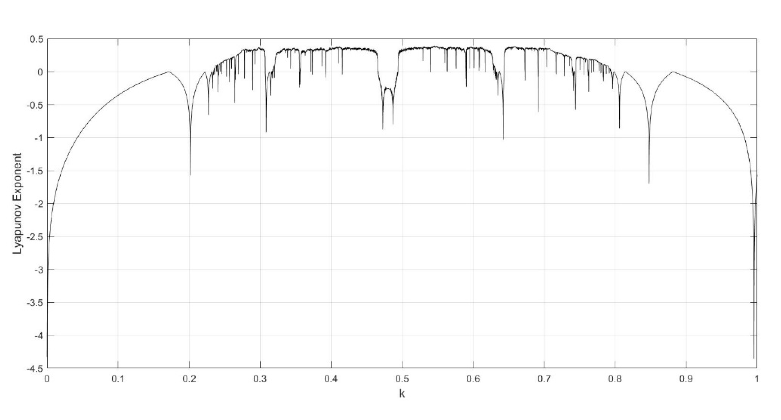
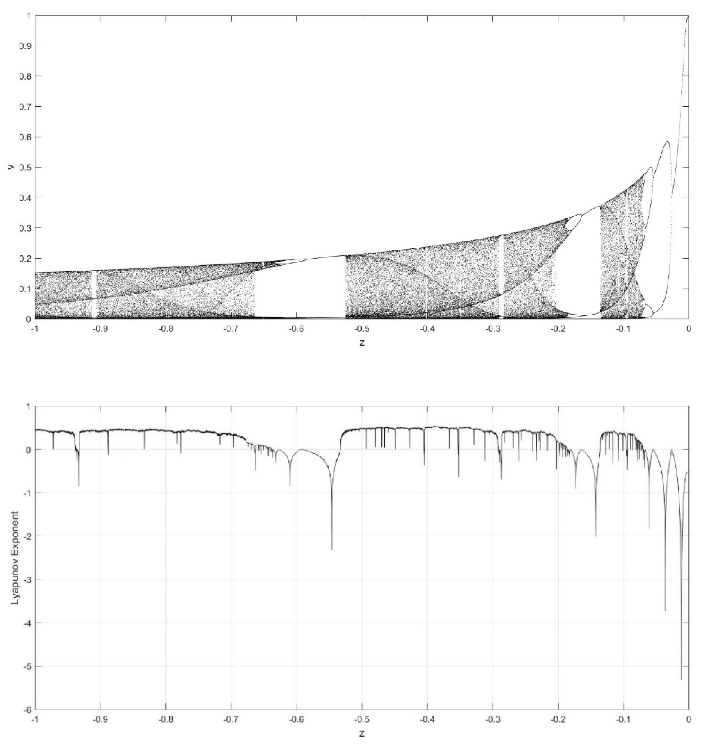
On the basis of Equations (8) and (9), it should be noted that the single neuronal dynamical system (SNDS) has four parameters. We can vary them to show complex dynamic behaviors. When the parameters hold specific value, a sequence of bifurcation leading to chaos can be observed by changing one parameter. To unmask the dynamical behavior of the SNDS, the single-parameter bifurcation diagrams and the corresponding evolution diagrams of the Lyapunov exponent are drawn, as shown in Figure 3, Figure 4, Figure 5 and Figure 6. In the figures, there is distinct correspondence between bifurcation diagrams and evolution diagrams of the Lyapunov exponent. For parameter , Figure 3 shows multiple instances of entering and exiting chaos, which are associated with multiple bifurcations phenomenon. The instances that exit chaos are sudden, and it corresponds to the sudden decrease of Lyapunov exponent in the evolution diagram. For parameter , as shown in Figure 4, it first gradually enters chaos, and then gradually exits after a period of evolution. In the evolution, chaos is not continuous. Furthermore, the Lyapunov exponent diagram of has symmetry in the domain of definition. Parameter also appears discontinuous chaos phenomenon in a large range, and parameter appears chaos phenomenon only within a very small range.
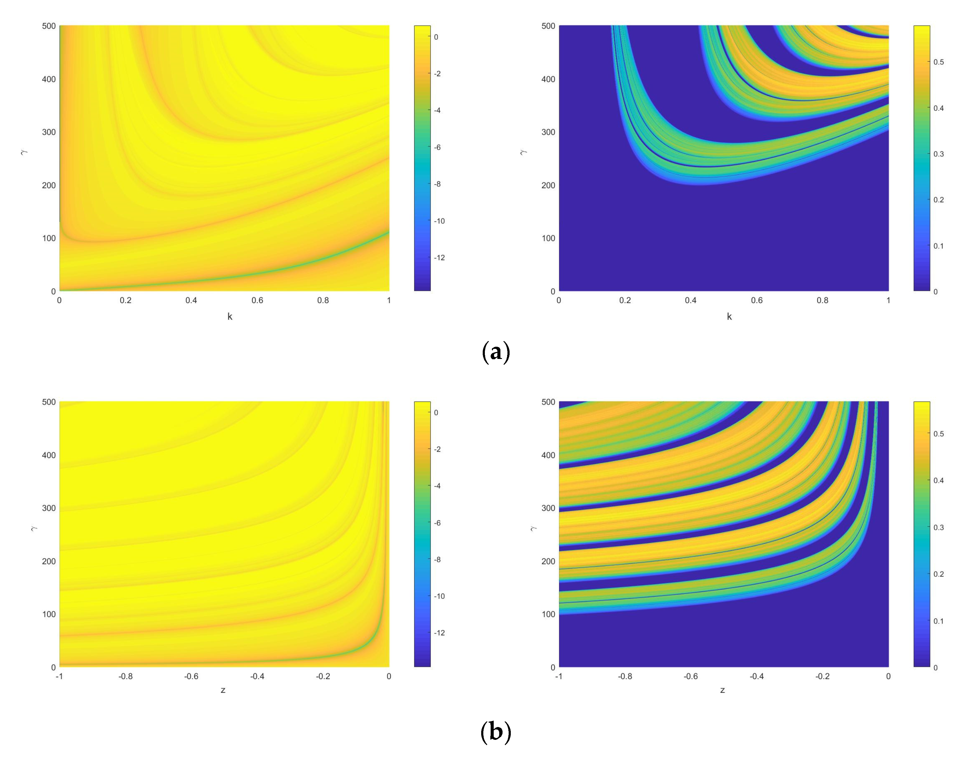
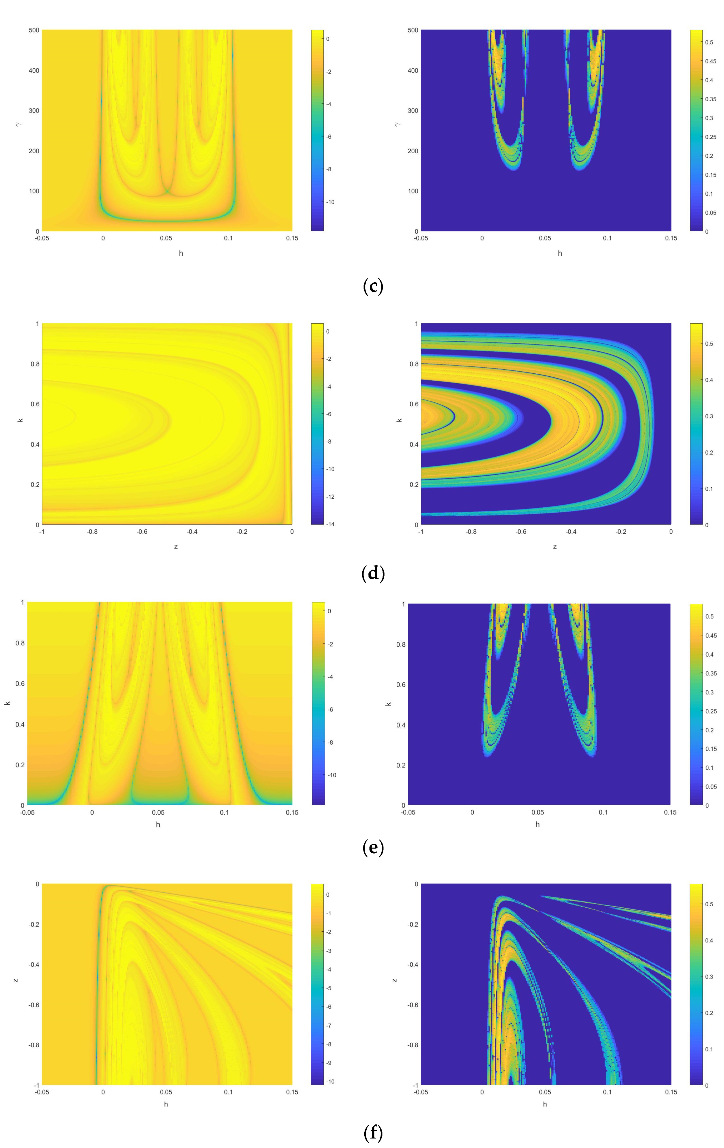
In addition, the double-parameter evolution diagrams of Lyapunov exponent are used for a clearer understanding of the dynamical behavior of SNDS, as shown in Figure 7. The Figure includes six parameter combinations. Each combination is presented by two two-dimensional evolution diagrams of Lyapunov exponent. The latter two-dimensional evolution diagram is formed on the basis of setting Lyapunov exponent which is less than zero to be zero. In Figure 7, some interesting phenomenon can be observed. The combinations of , , and appear wide area of chaos, and the area is banded in the diagram. This corresponds to the single-parameter evolution diagram of the Lyapunov exponent. On the contrary, the chaos range of the combination with parameter is narrow.
3.2. Efficiency Analysis
High efficiency of the chaotic map is necessary as practical applications always involve the generation of a large number of pseudorandom sequences. Compared with self-feedbacked Hopfield networks, SNDS has low implementation cost. Table 1 shows the time elapsed by SNDS and self-feedbacked Hopfield networks when generating pseudorandom sequences. The experimental environments are as follows: Matlab R2017a, Intel (R) Core (TM) i5-9400F CPU @ 2.90 GHz with 24 GB memory, Windows 10 Operation System. In the experiment, each sequence is generated 100 times, and the average running time is taken as the result. This indicates that SNDS has the higher efficiency than self-feedbacked Hopfield networks.
4. Enhanced Single Neuronal Dynamic System and Random Bit Generation
4.1. Enhanced Single Neuronal Dynamic System
By incorporating SNDS into the framework proposed in [54], The enhanced single neuronal dynamic system (ESNDS) is obtained. It is described by Equation (10):
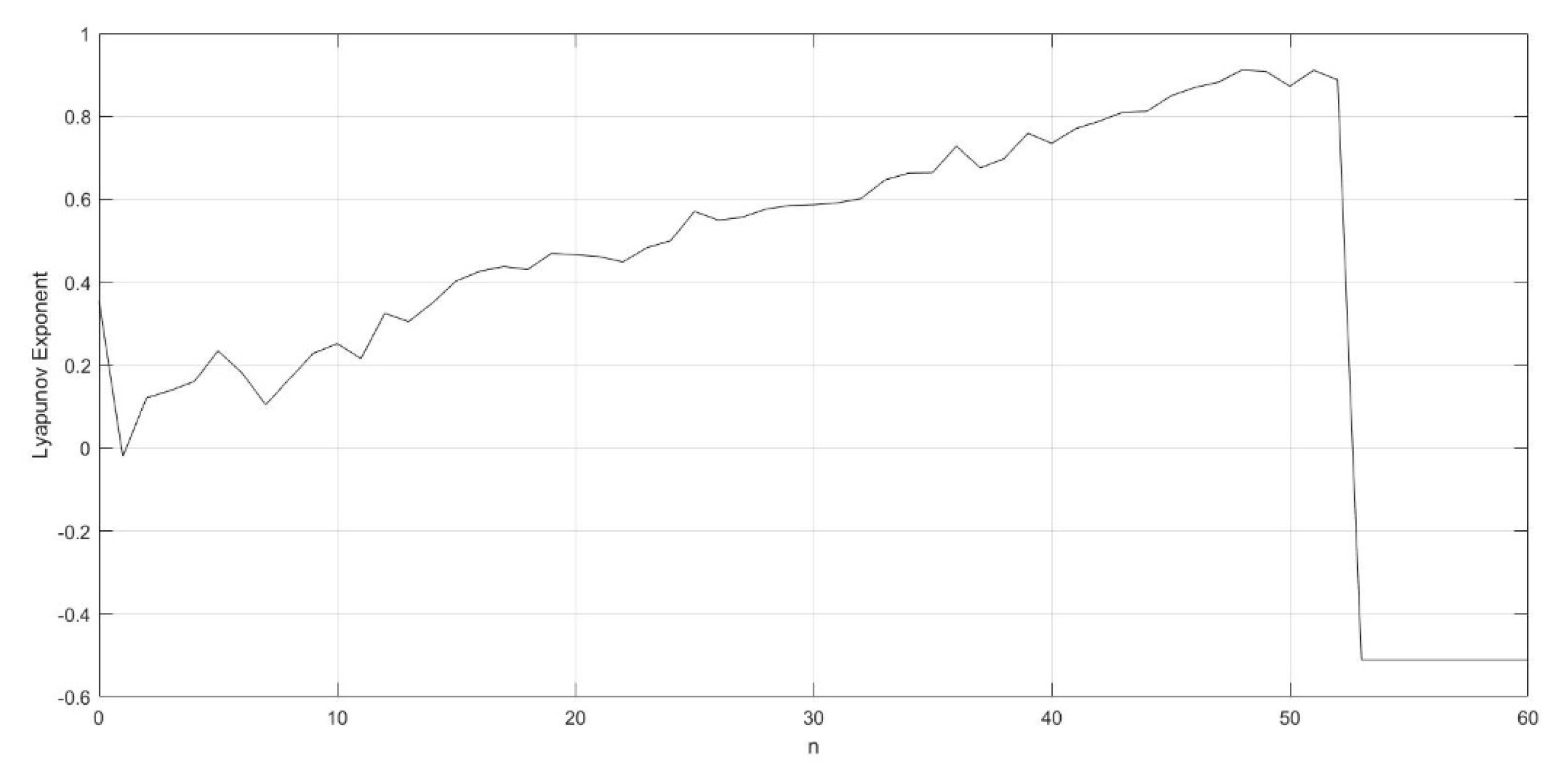
where the parameter is the value of after an intermediate calculation. The Lyapunov exponent evolution diagram of is shown as Figure 8. In this paper, is set to a fixed value of 14.
For ESNDS, the bifurcation diagrams and Lyapunov exponent evolution diagrams of single-parameter are shown in Figure 9, Figure 10, Figure 11 and Figure 12. It can be seen that the chaotic range of all parameters tends to be continuous. The Lyapunov exponent of Parameter falls first and rises later, and occurs around . The other three parameters are also in chaos over a wide range. Note that for , the chaotic property of this parameter has been greatly improved. It means that SNDS can achieve better performance by using the frameworks suitable for a simple chaotic system. This greatly increases the application potential of SNDS.
4.2. Random Bit Generation
4.2.1. NIST SP800-22 Test
To demonstrate the robustness of ESNDS and the potential of its application in image encryption, the NIST SP800-22 test standard is used for ESNDS. It is designed by National Institute of Standards and Technology (NIST) to validate the randomness of binary sequences [59]. NIST SP800-22 is the most complete statistical test suite for randomness test of binary sequences [60]. The binary numbers are generated by the value of in the iterative process of ESNDS. For each value of , we discard the former 10 decimal digits and compare the result with 0.5, the process is shown as Equations (11) and (12):
The NIST test standard includes 15 subsets. In the experiment, all subsets were considered, and each subset can output a p-value. If the p-value is greater than 0.01, the sequence is thought to pass a subset. The length of each binary sequence is 1,000,000 bits, and we test 100 binary sequences for each subset. During the process, the initial values of parameters for ESNDS are set as follows: , , , , and . The result is shown in Table 2, and of the last round is put into the table. According to [59], the minimum pass rate of each subset is 96 percent. Therefore, a dynamical system is chaotic enough if the minimum pass rate is achieved in all subsets.
4.2.2. TestU01
To further investigate the pseudo-random sequence generated by ESNDS, two binary sequences are used in TestU01. As an empirical statistical test suite, TestU01 can evaluate the randomness of sequences through a collection of utilities [61]. The length of two binary sequences is 30,000,000 bits and 1,000,000,000 bits, respectively. In standard tests suits, the sequence size of nearly 30,000,000 is commonly used [62,63]. In the experiment, three predefined batteries, Rabbit, Alphabit, and Block Alphabit, are used to evaluate the randomness of bits generated by ESNDS. The initial values of parameters for ESNDS are set as follows: , , , , and . The result is shown in Table 3. It can be seen that the sequences have strong randomness and ESNDS is effective.
4.2.3. The Sensitivity to Initial Condition
The sensitivity to initial condition is how slightly a parameter or initial value change will generate different sequence. In this section, the four parameters and initial value of ESNDS are studied. The result is shown in Figure 13. It is seen that the sequences vary at about ten iterations of all parameters and initial value. Therefore, ESNDS is sufficiently sensitive to initial condition and can fully ensure encryption security.
4.3. Performance Analysis
4.3.1. Sample Entropy
Sample Entropy (SE) is used to describe the complexity of a time series quantitatively [64]. The computing method of SE is defined in [65]. The time series with a lower degree of regularity always have a larger SE. Therefore, a lager SE indicates that the time series is higher complexity. In order to reflect the complexity of the sequences generated by ESNDS clearly, we introduced two simple chaotic maps (i.e., Sine map, Logistic map) and Two coupled chaotic maps which are proposed in [48,55]. The coupled chaotic map in [48] is defined as Equation (13), and that in [55] is defined as Equations (14) and (15).
For intuitive comparison, the parameters and are selected to depict the SE of ESNDS, as shown in Figure 14. Furthermore, Figure 14a includes the SE of coupled chaotic map in [55] along parameters and , and Figure 14b includes the SE of coupled chaotic map in [48] and simple chaotic maps along parameter . It can be seen that ESNDS have relatively wider chaotic range and larger SE than the simple chaotic maps and the coupled chaotic maps. This indicates that ESNDS can generate sequences with more complex properties. It is of significance for chaotic maps applied in data security.
4.3.2. Efficiency Analysis
In considering the complexity of sequences generated by chaotic maps, the high efficiency of chaotic maps is also necessary. The implementation cost of ESNDS is calculated in different length of sequence, and it is also compared with coupled chaotic maps proposed in [48,55], as shown in Table 4. In the experiment, each sequence is generated 100 times, and the average running time is taken as the result. It can be seen that implementation cost of ESNDS is in the middle of the three chaotic maps. Therefore, ESNDS is suitable for data security.
5. Application to Image Encryption
5.1. Encryption Process
Step 1: The original grayscale image is read as a matrix for further processing. In addition, each element in the matrix is an integer from 0 to 255.
Step 2: The chaotic sequence is obtained from the ESNDS for encryption. , , , and are initial values of ESNDS, so they are used as the security keys. Iterate the ESNDS times, and discard the former elements. Therefore, a new sequence with ) is obtained.
Step 3: Take the former elements as sequence , the next elements as sequence , and the rest elements as sequence . The following modifications were made to sequence and , as Equation (16):
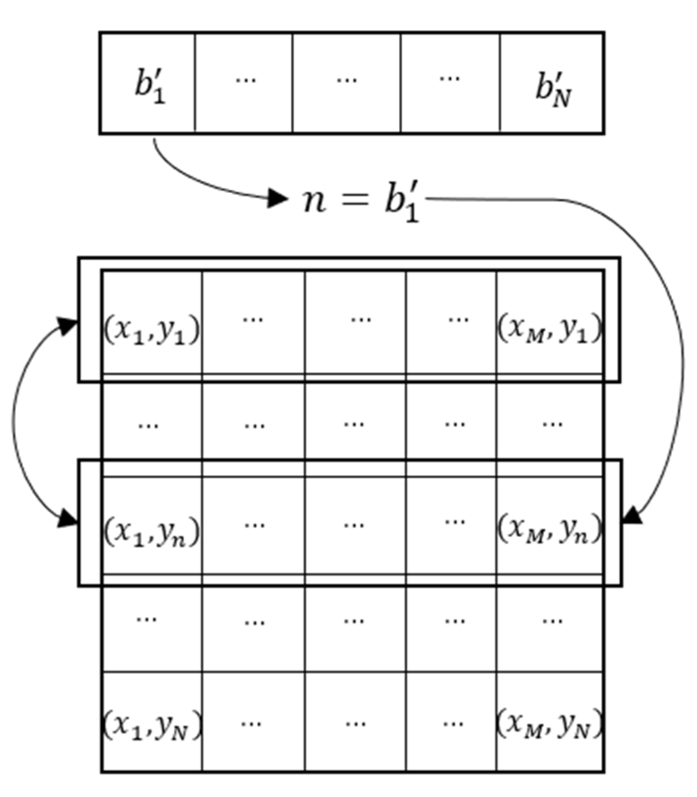
Step 4: Obtain the column permutation matrix. The process is shown in Figure 15.
Step 5: Obtain the row permutation matrix. The process is shown in Figure 16.
Step 6: The permutated matrix is converted into the 1D matrix , and sort the sequence in ascending order. According to the sorting result, matrix is obtained. The process is shown in Figure 17.
Step 7: Obtain the diffused matrix from the sequence and the matrix by Equations (17) and (18):
Step8: Convert into the encrypted image with the size of .
The decryption is the inverse process of encryption.
In the experiment, the initial value of ESNDS , the parameters , , , , and four images are used to verify encryption effect of the encryption method. The original images and results of encryption are shown in Figure 18.
5.2. Security Analysis
5.2.1. Security Key Space
Key space refers to the summation of the different keys that can be used for encryption. Due to multiple parameters of ESNDS, it is very complicated to determine the range of all the keys that can generate chaotic sequences simultaneously. Therefore, we confirm the range of some parameters by the two-dimensional diagram of Lyapunov exponent to determine the minimum key space. The two-dimensional evolution diagram of Lyapunov exponent of is shown as Figure 19. Figure 19 and Section 4.2.2 show that the both space of and is about , and the space of is . We can get the minimum key space is . The minimum key space is larger than which enough to resist brute force attacks [66,67].
5.2.2. Information Entropy
The information entropy is a measurement standard of the degree of information ordering in digital images [68]. It is defined as Equation (19):
where represents the grayscale level of an image, and represents the probability of the grayscale value . For a completely random image, the theoretical value of information entropy is 8 [69]. As shown in Table 5, the information entropy of encrypted images is close to the theoretical value. It shows the degree of information ordering tends to disorder after the encryption scheme.
5.2.3. Correlation Analysis
In plaintext images, adjacent pixels tend to have high correlations. This is related to the discernibility of the information in the images. Therefore, it is necessary to reduce the correlation between adjacent pixels in the encrypted images [70]. The equation is shown as Equation (20):
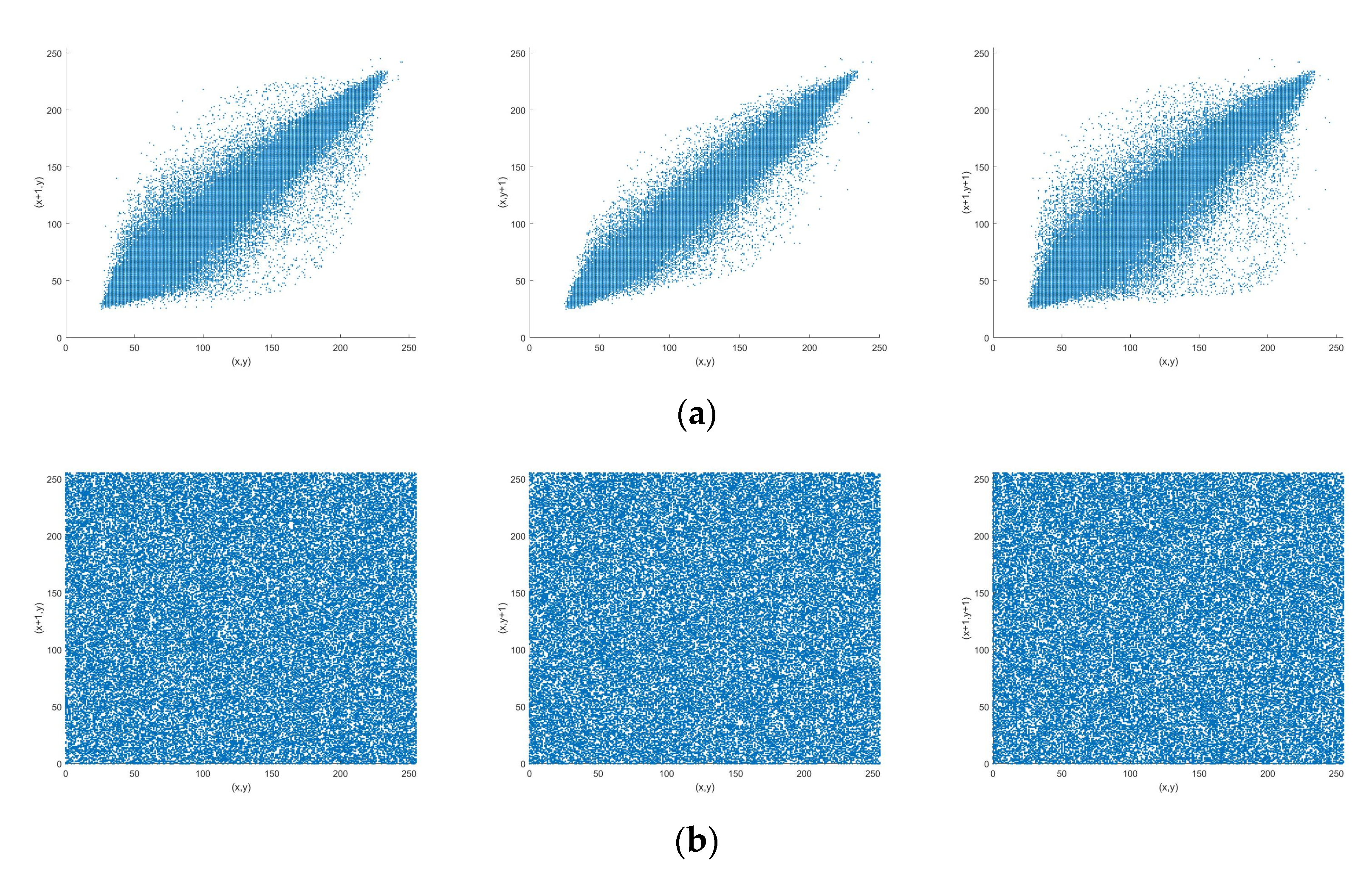
where, and are the gray values of adjacent pixels, and represents the correlation coefficient between adjacent pixels. The horizontal, vertical and diagonal correlation of original image Lena and encrypted image Lena is shown in Figure 20. As shown in Table 6, compared with original images, the correlation coefficient of encrypted images is greatly reduced. This means that the encrypted images effectively conceal the information of the original images. In addition, Table 7 demonstrates the correlation coefficient of encrypted Lena using various encryption schemes. It can be seen that our scheme achieves relatively favorable performance among these methods.
5.2.4. Sensitivity Analysis
A good encryption scheme should be sensitive to tiny changes in key and plaintext image. To test the sensitivity of the proposed scheme, two with only differences are used to encrypt the original images, respectively. The difference between two encrypted images can be measured through the Number of Pixel Change Rate (NPCR) and the Unified Average Changing Intensity (UACI). The NPCR and UACI are calculated by Equations (21) and (22) [72]:
where and are two images with the size of . If , then , otherwise, . According to [77], the expected value of NPCR and UACI are 99.6094% and 33.4635% for 8-bit grayscale images. Table 8 shows the value of NPCR and UACI of four images. It can be seen that the proposed encryption scheme is sensitive to tiny changes in key.
5.2.5. Histogram Analysis
The histogram analysis refers to the number of times each value appears, so as to reflect the distribution of pixel values of an image [21]. The ideal histogram should be flat and smooth to resist statistic attacks. The Figure 21 shows the histograms of four original images and the histograms of corresponding encrypted images. The pixel value distribution of the four encrypted images is uniform, so it can resist statistic attacks.
5.2.6. Noise Robustness
Due to noise attack or noise jamming in the transmission channel, the pixel value modification of cipher images may appear [78,79]. The noise makes the information in cipher images difficult to recover. However, receivers would like to recover the original images as much as possible in the situation. Thus, an encryption scheme should have an ability of resisting noise.
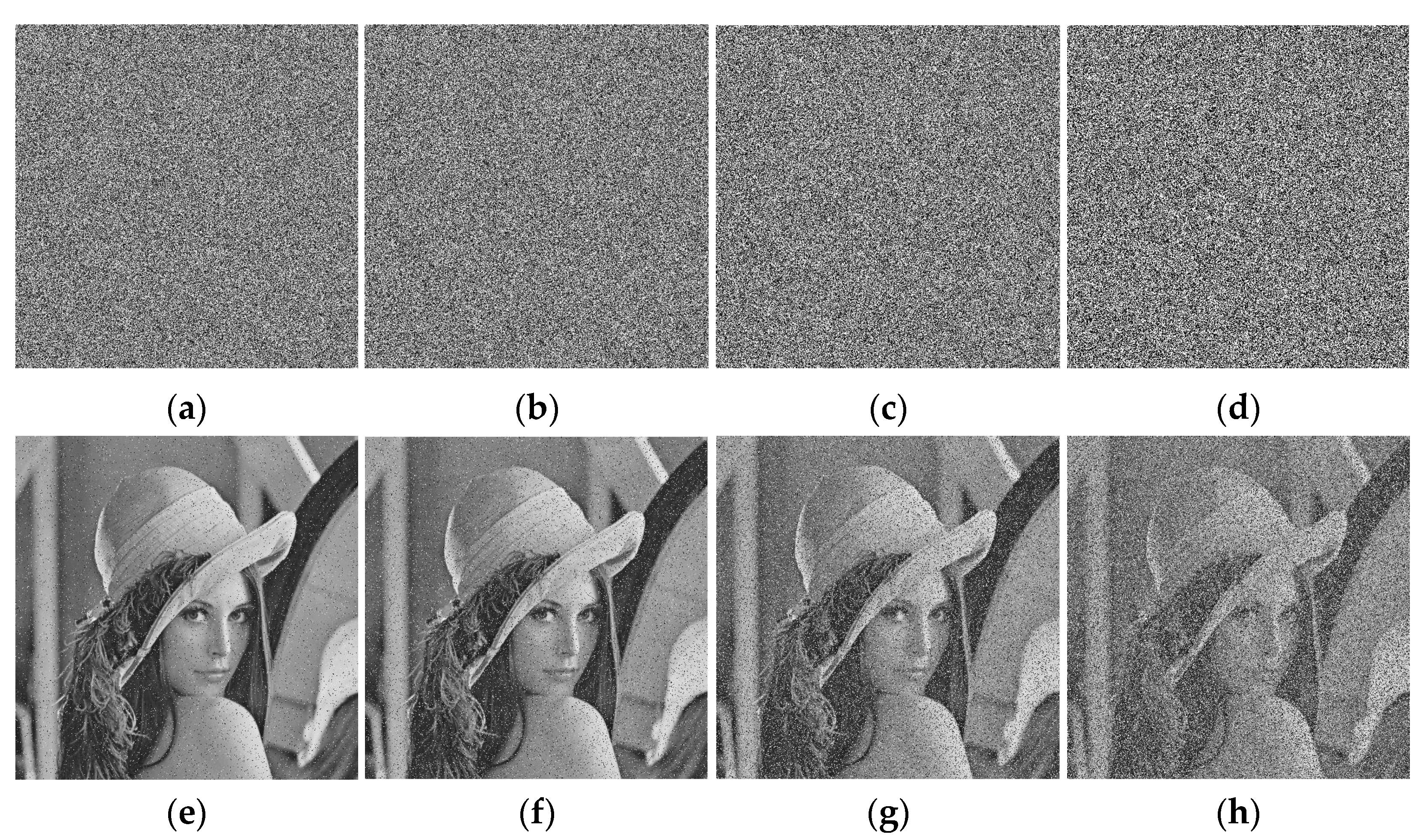
To test the ability of resisting noise, an experiment on noise attack is performed. Four different proportions of ‘salt & pepper’ noise are added to the encrypted Lena. The decryption process is then applied to the images with “salt & pepper” noise. The results are shown in Figure 22. It can be seen that the decrypted images recover most information of the original images.
5.2.7. Robustness to Data Loss
In practical application, digital images are vulnerable to data loss in the process of communication for all kind of reason. This may be caused by the various interception, and some parts of digital images may be missing. In this case, the receiver can be easily failed to get the intact data. To cope with this, the encrypted images should have good anti-cutting performance.
Our proposed encryption scheme has enough robustness to data loss. The data loss is performed at the rate of 25% and 50% in different positions, and the processed images are used for decryption. The results are shown in Figure 23. It can be seen that the decrypted images restore most of the original details visually. This shows the encryption scheme has enough robustness to data loss.
5.3. Speed Analysis
Since the proposed encryption scheme is a kind of symmetric encryption scheme, the decryption is the inverse process of encryption. We only analyze the encryption speed in this section.
For the time complexity analysis of the scheme, the time-consuming part includes floating-point operations for the construction of chaotic sequences in ESNDS and permutation-diffusion process. Table 9 lists the computational complexity of the proposed encryption scheme as well as some other chaos-based image encryption schemes. The efficiency of the proposed scheme is comparable with existing chaos-based ciphers.
Furthermore, the speed of the encryption scheme is tested. The experimental environment is same as that in Section 3.2. The images with different size are encrypted, and the running time is shown in Table 10. In the experiment, each encryption is repeated 100 times, and the average running time is taken as the result. It can be seen that the average encryption/decryption speed of proposed scheme is enough for image encryption applications.
6. Conclusions
In this paper, the single neuronal dynamical system in self-feedbacked Hopfield network is proposed, and its derivation process of the discrete form is given. The chaotic dynamic behavior of the system is described from single-parameter and double-parameter perspectives. The implementation cost of the system is also lower than self-feedbacked Hopfield networks. Furthermore, we apply a framework for improving chaotic properties of the simple chaotic system to our system and achieve good performance. It is important to note that this applicability can make for the system being considered in more fields. In addition, an image encryption scheme based on the enhanced system is herein designed. The simulation results and security analysis prove that the scheme has an excellent performance.
The single neuronal dynamical system in self-feedbacked Hopfield Networks still has a large scope for exploration. In future work, we will continue improving the system, such as changing the activation function.
Author Contributions
Conceptualization, X.X.; Methodology, X.X.; Software, X.X.; Visualization, X.X.; Writing, X.X.; Supervision, S.C.; Validation, S.C. All authors have read and agreed to the published version of the manuscript.
Funding
This research was funded by Jilin province and Jilin university co-building project, grant number SXGJXX2017-2; and the program for JLU science and technology innovative research team, grant number JLUSTIRT, 2017TD-26.
Data Availability Statement
Not applicable.
Acknowledgments
We thank the editors and the reviewers for their constructive suggestions and insightful comments, which helped us greatly to improve this manuscript.
Conflicts of Interest
The authors declare no conflict of interest.
References
- Fradkov, A.L.; Evans, R.J. Control of chaos: Methods and applications in engineering. Annu. Rev. Control 2005, 29, 33–56. [Google Scholar] [CrossRef]
- Kiani, B.A.; Fallahi, K.; Pariz, N.; Leung, H. A chaotic secure communication scheme using fractional chaotic systems based on an extended fractional Kalman filter. Commun. Nonlinear Sci. Numer. Simul. 2009, 14, 863–879. [Google Scholar] [CrossRef]
- Mead, C. Neuromorphic electronic systems. Proc. IEEE 1990, 78, 1629–1636. [Google Scholar] [CrossRef] [Green Version]
- Pickett, M.D.; Williams, R.S. Phase transitions enable computational universality in neuristor-based cellular automata. Nanotechnology 2013, 24, 384002. [Google Scholar] [CrossRef] [PubMed] [Green Version]
- Volos, C.K.; Kyprianidis, I.M.; Stouboulos, I.N. Image encryption process based on chaotic synchronization phenomena. Signal Process. 2013, 93, 1328–1340. [Google Scholar] [CrossRef]
- Yang, J.; Wang, L.; Wang, Y.; Guo, T. A novel memristive Hopfield neural network with application in associative memory. Neurocomputing 2017, 227, 142–148. [Google Scholar] [CrossRef]
- Hopfield, J.J. Neural networks and physical systems with emergent collective computational abilities. Proc. Natl. Acad. Sci. USA 1982, 79, 2554–2558. [Google Scholar] [CrossRef] [Green Version]
- Hopfield, J.J. Neurons with graded response have collective computational properties like those of two-state neurons. Proc. Natl. Acad. Sci. USA 1984, 81, 3088–3092. [Google Scholar] [CrossRef] [Green Version]
- Lázaro, O.; Girma, D. A Hopfield neural-network-based dynamic channel allocation with handoff channel reservation control. Ieee Trans. Veh. Technol. 2000, 49, 1578–1587. [Google Scholar] [CrossRef]
- Wilson, G.; Pawley, G. On the stability of the travelling salesman problem algorithm of Hopfield and Tank. Biol. Cybern. 1988, 58, 63–70. [Google Scholar] [CrossRef]
- Aiyer, S.V.; Niranjan, M.; Fallside, F. A theoretical investigation into the performance of the Hopfield model. IEEE Trans. Neural Netw. 1990, 1, 204–215. [Google Scholar] [CrossRef] [PubMed]
- Van den Bout, D.E.; Miller, T. Improving the performance of the Hopfield-Tank neural network through normalization and annealing. Biol. Cybern. 1989, 62, 129–139. [Google Scholar] [CrossRef]
- Yoshino, K. Hopfield neural network using oscillatory units with sigmoidal input-average out characteristics. IEICE Trans. 1994, 77, 219–227. [Google Scholar]
- Watanabe, Y.; Yoshino, K.; Kakeshita, T. Solving combinatorial optimization problems using the oscillatory neural network. IEICE Trans. Inf. Syst. 1997, 80, 72–77. [Google Scholar]
- Li, Y.; Tang, Z.; Wang, R.L.; Xia, G.; Xu, X. A fast and reliable approach to TSP using positively self-feedbacked hopfield networks. IEEJ Trans. Electron. Inf. Syst. 2004, 124, 2353–2358. [Google Scholar] [CrossRef] [Green Version]
- Danca, M.-F.; Kuznetsov, N. Hidden chaotic sets in a Hopfield neural system. Chaos Solitons Fractals 2017, 103, 144–150. [Google Scholar] [CrossRef]
- Li, Y.; Tang, Z.; Xia, G.; Wang, R. A positively self-feedbacked Hopfield neural network architecture for crossbar switching. IEEE Trans. Circuits Syst. I Regul. Pap. 2005, 52, 200–206. [Google Scholar]
- Liu, L.; Zhang, L.; Jiang, D.; Guan, Y.; Zhang, Z. A simultaneous scrambling and diffusion color image encryption algorithm based on Hopfield chaotic neural network. IEEE Access 2019, 7, 19. [Google Scholar] [CrossRef]
- Bigdeli, N.; Farid, Y.; Afshar, K. A robust hybrid method for image encryption based on Hopfield neural network. Comput. Electr. Eng. 2012, 38, 356–369. [Google Scholar] [CrossRef]
- Hu, Y.; Yu, S.; Zhang, Z. On the Security Analysis of a Hopfield Chaotic Neural Network-Based Image Encryption Algorithm. Complexity 2020, 2020. [Google Scholar] [CrossRef]
- Wang, X.-Y.; Li, Z.-M. A color image encryption algorithm based on Hopfield chaotic neural network. Opt. Lasers Eng. 2019, 115, 107–118. [Google Scholar] [CrossRef]
- Tlelo-Cuautle, E.; Díaz-Muñoz, J.D.; González-Zapata, A.M.; Li, R.; León-Salas, W.D.; Fernández, F.V.; Guillén-Fernández, O.; Cruz-Vega, I. Chaotic image encryption using hopfield and hindmarsh–rose neurons implemented on FPGA. Sensors 2020, 20, 1326. [Google Scholar] [CrossRef] [PubMed] [Green Version]
- Ding, Y.; Dong, L.; Zhao, B.; Lu, Z. High Order Hopfield Network with Self-feedback to Solve Crossbar Switch Problem. In Proceedings of the International Conference on Neural Information Processing, Shanghai, China, 13–17 November 2011; Springer: Berlin/Heidelberg, Germany, 2011; pp. 315–322. [Google Scholar]
- Wang, J.; Yi, W. Nonpositive hopfield neural network with self-feedback and its application to maximum clique problems. Neural Inf. Process. Lett. Rev. 2006, 10. [Google Scholar]
- Zhu, S.; Zhu, C.; Cui, H.; Wang, W. A class of quadratic polynomial chaotic maps and its application in cryptography. IEEE Access 2019, 7, 34141–34152. [Google Scholar] [CrossRef]
- Zhu, S.; Zhu, C.; Wang, W. A new image encryption algorithm based on chaos and secure hash SHA-256. Entropy 2018, 20, 716. [Google Scholar] [CrossRef] [Green Version]
- de la Fraga, L.G.; Torres-Pérez, E.; Tlelo-Cuautle, E.; Mancillas-López, C. Hardware implementation of pseudo-random number generators based on chaotic maps. Nonlinear Dyn. 2017, 90, 1661–1670. [Google Scholar] [CrossRef]
- Ullah, A.; Jamal, S.S.; Shah, T. A novel construction of substitution box using a combination of chaotic maps with improved chaotic range. Nonlinear Dyn. 2017, 88, 2757–2769. [Google Scholar] [CrossRef]
- Belazi, A.; Khan, M.; Abd El-Latif, A.A.; Belghith, S. Efficient cryptosystem approaches: S-boxes and permutation–substitution-based encryption. Nonlinear Dyn. 2017, 87, 337–361. [Google Scholar] [CrossRef]
- Del Rey, A.M.; Sánchez, G.R. An image encryption algorithm based on 3D cellular automata and chaotic maps. Int. J. Mod. Phys. C 2015, 26, 1450069. [Google Scholar] [CrossRef]
- Chai, X.-L.; Gan, Z.-H.; Yuan, K.; Lu, Y.; Chen, Y.-R. An image encryption scheme based on three-dimensional Brownian motion and chaotic system. Chin. Phys. B 2017, 26, 020504. [Google Scholar] [CrossRef]
- Wu, G.-C.; Baleanu, D. Discrete fractional logistic map and its chaos. Nonlinear Dyn. 2014, 75, 283–287. [Google Scholar] [CrossRef]
- Wang, Y.; Liu, Z.; Ma, J.; He, H. A pseudorandom number generator based on piecewise logistic map. Nonlinear Dyn. 2016, 83, 2373–2391. [Google Scholar] [CrossRef]
- Liu, L.; Miao, S.; Cheng, M.; Gao, X. A pseudorandom bit generator based on new multi-delayed Chebyshev map. Inf. Process. Lett. 2016, 116, 674–681. [Google Scholar] [CrossRef]
- Pareek, N.K.; Patidar, V.; Sud, K.K. Image encryption using chaotic logistic map. Image Vis. Comput. 2006, 24, 926–934. [Google Scholar] [CrossRef]
- Borujeni, S.E.; Ehsani, M.S. Modified logistic maps for cryptographic application. Appl. Math. 2015, 6, 773. [Google Scholar] [CrossRef] [Green Version]
- Belazi, A.; Abd El-Latif, A.A. A simple yet efficient S-box method based on chaotic sine map. Optik 2017, 130, 1438–1444. [Google Scholar] [CrossRef]
- Ye, G.; Huang, X. An efficient symmetric image encryption algorithm based on an intertwining logistic map. Neurocomputing 2017, 251, 45–53. [Google Scholar] [CrossRef]
- Li, C.; Xie, T.; Liu, Q.; Cheng, G. Cryptanalyzing image encryption using chaotic logistic map. Nonlinear Dyn. 2014, 78, 1545–1551. [Google Scholar] [CrossRef] [Green Version]
- Ye, G. Image scrambling encryption algorithm of pixel bit based on chaos map. Pattern Recognit. Lett. 2010, 31, 347–354. [Google Scholar] [CrossRef]
- Arroyo, D.; Rhouma, R.; Alvarez, G.; Li, S.; Fernandez, V. On the security of a new image encryption scheme based on chaotic map lattices. Chaos Interdiscip. J. Nonlinear Sci. 2008, 18, 033112. [Google Scholar] [CrossRef] [Green Version]
- Wu, X.; Hu, H.; Zhang, B. Parameter estimation only from the symbolic sequences generated by chaos system. ChaosSolitons Fractals 2004, 22, 359–366. [Google Scholar] [CrossRef]
- Li, C.; Arroyo, D.; Lo, K.-T. Breaking a chaotic cryptographic scheme based on composition maps. Int. J. Bifurc. Chaos 2010, 20, 2561–2568. [Google Scholar] [CrossRef] [Green Version]
- Li, C.; Liu, Y.; Zhang, L.Y.; Chen, M.Z. Breaking a chaotic image encryption algorithm based on modulo addition and XOR operation. Int. J. Bifurc. Chaos 2013, 23, 1350075. [Google Scholar] [CrossRef] [Green Version]
- Li, C.; Feng, B.; Li, S.; Kurths, J.; Chen, G. Dynamic analysis of digital chaotic maps via state-mapping networks. IEEE Trans. Circuits Syst. I Regul. Pap. 2019, 66, 2322–2335. [Google Scholar] [CrossRef] [Green Version]
- Hua, Z.; Zhou, Y.; Pun, C.-M.; Chen, C.P. 2D Sine Logistic modulation map for image encryption. Inf. Sci. 2015, 297, 80–94. [Google Scholar] [CrossRef]
- Song, C.-Y.; Qiao, Y.-L.; Zhang, X.-Z. An image encryption scheme based on new spatiotemporal chaos. Opt. Int. J. Light Electron Opt. 2013, 124, 3329–3334. [Google Scholar] [CrossRef]
- Hua, Z.; Zhou, Y. Image encryption using 2D Logistic-adjusted-Sine map. Inf. Sci. 2016, 339, 237–253. [Google Scholar] [CrossRef]
- Mansouri, A.; Wang, X. A novel one-dimensional sine powered chaotic map and its application in a new image encryption scheme. Inf. Sci. 2020, 520, 46–62. [Google Scholar] [CrossRef]
- Lv-Chen, C.; Yu-Ling, L.; Sen-Hui, Q.; Jun-Xiu, L. A perturbation method to the tent map based on Lyapunov exponent and its application. Chin. Phys. B 2015, 24, 100501. [Google Scholar]
- Zhou, Y.; Bao, L.; Chen, C.P. A new 1D chaotic system for image encryption. Signal Process. 2014, 97, 172–182. [Google Scholar] [CrossRef]
- Wen, W.; Zhang, Y.; Fang, Z.; Chen, J.-x. Infrared target-based selective encryption by chaotic maps. Opt. Commun. 2015, 341, 131–139. [Google Scholar] [CrossRef]
- Abd El-Latif, A.A.; Niu, X. A hybrid chaotic system and cyclic elliptic curve for image encryption. Aeu-Int. J. Electron. Commun. 2013, 67, 136–143. [Google Scholar] [CrossRef]
- Pak, C.; Huang, L. A new color image encryption using combination of the 1D chaotic map. Signal Process. 2017, 138, 129–137. [Google Scholar] [CrossRef]
- Moysis, L.; Volos, C.; Jafari, S.; Munoz-Pacheco, J.M.; Kengne, J.; Rajagopal, K.; Stouboulos, I. Modification of the logistic map using fuzzy numbers with application to pseudorandom number generation and image encryption. Entropy 2020, 22, 474. [Google Scholar] [CrossRef] [Green Version]
- Hu, G.; Li, B. Coupling chaotic system based on unit transform and its applications in image encryption. Signal Process. 2021, 178, 107790. [Google Scholar] [CrossRef]
- Alawida, M.; Samsudin, A.; Teh, J.S. Enhanced digital chaotic maps based on bit reversal with applications in random bit generators. Inf. Sci. 2020, 512, 1155–1169. [Google Scholar] [CrossRef]
- Chen, C.; Sun, K.; He, S. An improved image encryption algorithm with finite computing precision. Signal Process. 2020, 168, 107340. [Google Scholar] [CrossRef]
- Bassham, L.E., III; Rukhin, A.L.; Soto, J.; Nechvatal, J.R.; Smid, M.E.; Barker, E.B.; Leigh, S.D.; Levenson, M.; Vangel, M.; Banks, D.L. Sp 800-22 Rev. 1a. a Statistical Test Suite for Random and Pseudorandom Number Generators for Cryptographic Applications; National Institute of Standards & Technology: Gaithersburg, MD, USA, 2010.
- Meranza-Castillón, M.; Murillo-Escobar, M.; López-Gutiérrez, R.; Cruz-Hernández, C. Pseudorandom number generator based on enhanced Hénon map and its implementation. Aeu-Int. J. Electron. Commun. 2019, 107, 239–251. [Google Scholar] [CrossRef]
- Simard, R. TestU01: AC Library for Empirical Testing of Random Number Generators P. L’Ecuyer. Les Cah. Du Gerad Issn 2006, 711, 2440. [Google Scholar]
- Lambić, D.; Nikolić, M. Pseudo-random number generator based on discrete-space chaotic map. Nonlinear Dyn. 2017, 90, 223–232. [Google Scholar] [CrossRef]
- Marangon, D.G.; Vallone, G.; Villoresi, P. Random bits, true and unbiased, from atmospheric turbulence. Sci. Rep. 2014, 4, 1–8. [Google Scholar] [CrossRef] [Green Version]
- Richman, J.S.; Moorman, J.R. Physiological time-series analysis using approximate entropy and sample entropy. Am. J. Physiol. Heart Circ. Physiol. 2000. [Google Scholar] [CrossRef] [Green Version]
- Hua, Z.; Zhou, Y.; Huang, H. Cosine-transform-based chaotic system for image encryption. Inf. Sci. 2019, 480, 403–419. [Google Scholar] [CrossRef]
- François, M.; Grosges, T.; Barchiesi, D.; Erra, R. Pseudo-random number generator based on mixing of three chaotic maps. Commun. Nonlinear Sci. Numer. Simul. 2014, 19, 887–895. [Google Scholar] [CrossRef]
- François, M.; Grosges, T.; Barchiesi, D.; Erra, R. A new image encryption scheme based on a chaotic function. Signal Process. Image Commun. 2012, 27, 249–259. [Google Scholar] [CrossRef]
- Hang, S.; Li-Dan, W. Multi-process image encryption scheme based on compressed sensing and multi-dimensional chaotic system. Acta Phys. Sin. 2019, 68, 200501. [Google Scholar] [CrossRef]
- Wei, X.; Guo, L.; Zhang, Q.; Zhang, J.; Lian, S. A novel color image encryption algorithm based on DNA sequence operation and hyper-chaotic system. J. Syst. Softw. 2012, 85, 290–299. [Google Scholar] [CrossRef]
- Behnia, S.; Akhshani, A.; Mahmodi, H.; Akhavan, A. A novel algorithm for image encryption based on mixture of chaotic maps. Chaos Solitons Fractals 2008, 35, 408–419. [Google Scholar] [CrossRef]
- Alawida, M.; Samsudin, A.; Teh, J.S.; Alkhawaldeh, R.S. A new hybrid digital chaotic system with applications in image encryption. Signal Process. 2019, 160, 45–58. [Google Scholar] [CrossRef]
- Wang, X.; Liu, L.; Zhang, Y. A novel chaotic block image encryption algorithm based on dynamic random growth technique. Opt. Lasers Eng. 2015, 66, 10–18. [Google Scholar] [CrossRef]
- Liu, W.; Sun, K.; Zhu, C. A fast image encryption algorithm based on chaotic map. Opt. Lasers Eng. 2016, 84, 26–36. [Google Scholar] [CrossRef]
- Gayathri, J.; Subashini, S. An efficient spatiotemporal chaotic image cipher with an improved scrambling algorithm driven by dynamic diffusion phase. Inf. Sci. 2019, 489, 227–254. [Google Scholar] [CrossRef]
- Diaconu, A.-V. Circular inter–intra pixels bit-level permutation and chaos-based image encryption. Inf. Sci. 2016, 355, 314–327. [Google Scholar] [CrossRef]
- Xu, L.; Li, Z.; Li, J.; Hua, W. A novel bit-level image encryption algorithm based on chaotic maps. Opt. Lasers Eng. 2016, 78, 17–25. [Google Scholar] [CrossRef]
- Wu, Y.; Noonan, J.P.; Agaian, S. NPCR and UACI randomness tests for image encryption. Cyber J. Multidiscip. J. Sci. Technol. J. Sel. Areas Telecommun. JSAT 2011, 1, 31–38. [Google Scholar]
- Alvarez, G.; Li, S. Some basic cryptographic requirements for chaos-based cryptosystems. Int. J. Bifurc. Chaos 2006, 16, 2129–2151. [Google Scholar] [CrossRef] [Green Version]
- Murillo-Escobar, M.A.; Meranza-Castillón, M.O.; López-Gutiérrez, R.M.; Cruz-Hernández, C. Suggested integral analysis for chaos-based image cryptosystems. Entropy 2019, 21, 815. [Google Scholar] [CrossRef] [Green Version]
Figure 1.
The structure of conventional Hopfield network [8].
Figure 1.
The structure of conventional Hopfield network [8].

Figure 2.
The structure of positively self-feedbacked Hopfield network [15].
Figure 2.
The structure of positively self-feedbacked Hopfield network [15].

Figure 3.
Single-parameter bifurcation diagram of versus parameter and corresponding Lyapunov exponent diagram for , , and .
Figure 3.
Single-parameter bifurcation diagram of versus parameter and corresponding Lyapunov exponent diagram for , , and .

Figure 4.
Single-parameter bifurcation diagram of versus parameter and corresponding Lyapunov exponent diagram for , , and .
Figure 4.
Single-parameter bifurcation diagram of versus parameter and corresponding Lyapunov exponent diagram for , , and .


Figure 5.
Single-parameter bifurcation diagram of versus parameter and corresponding Lyapunov exponent diagram for , , and .
Figure 5.
Single-parameter bifurcation diagram of versus parameter and corresponding Lyapunov exponent diagram for , , and .

Figure 6.
Single-parameter bifurcation diagram of versus parameter and corresponding Lyapunov exponent diagram for , , and .
Figure 6.
Single-parameter bifurcation diagram of versus parameter and corresponding Lyapunov exponent diagram for , , and .

Figure 7.
Two-dimensional evolution diagram of Lyapunov exponent (the original), and two-dimensional evolution diagram of Lyapunov exponent (set to ) of (a) - for and ; (b) - for and ; (c) - for and ; (d) - for and ; (e) - for and ; (f) - for and .
Figure 7.
Two-dimensional evolution diagram of Lyapunov exponent (the original), and two-dimensional evolution diagram of Lyapunov exponent (set to ) of (a) - for and ; (b) - for and ; (c) - for and ; (d) - for and ; (e) - for and ; (f) - for and .


Figure 8.
The evolution diagram of Lyapunov exponent versus parameter for , , , and .

Figure 9.
Single-parameter bifurcation diagram of versus parameter and corresponding Lyapunov exponent diagram for , , and .
Figure 9.
Single-parameter bifurcation diagram of versus parameter and corresponding Lyapunov exponent diagram for , , and .

Figure 10.
Single-parameter bifurcation diagram of versus parameter and corresponding Lyapunov exponent diagram for , , and .
Figure 10.
Single-parameter bifurcation diagram of versus parameter and corresponding Lyapunov exponent diagram for , , and .


Figure 11.
Single-parameter bifurcation diagram of versus parameter and corresponding Lyapunov exponent diagram for , , and .
Figure 11.
Single-parameter bifurcation diagram of versus parameter and corresponding Lyapunov exponent diagram for , , and .

Figure 12.
Single-parameter bifurcation diagram of versus parameter and corresponding Lyapunov exponent diagram for , , and .
Figure 12.
Single-parameter bifurcation diagram of versus parameter and corresponding Lyapunov exponent diagram for , , and .

Figure 13.
Sensitivity to initial condition of (a) varied initial value, for , , , ; (b) varied , for , , , ; (c) varied , for , , , ; (d) varied , for , , , ; (e) varied , for , , , .
Figure 13.
Sensitivity to initial condition of (a) varied initial value, for , , , ; (b) varied , for , , , ; (c) varied , for , , , ; (d) varied , for , , , ; (e) varied , for , , , .


Figure 14.
Comparison of SE between different maps: (a) ESNDS (z + 1) with , , , ESNDS (k) with , , , [55] ( ) with , and [55] ( ) with ; (b) ESNDS (z+1) with , , , ESNDS (k) with , , , [48] (), Sine map (), and Logistic map ().

Figure 15.
Matrix permutating process of column.

Figure 16.
Matrix permutating process of row.

Figure 17.
Permutating process of matrix .

Figure 18.
Encryption result of some images. (a) the original images; (b) the encrypted images.


Figure 19.
Two-dimensional evolution diagram of Lyapunov exponent (set to ) of for , .

Figure 20.
Correlation analysis of image Lena. (a) horizontal, vertical and diagonal correlation of original image; (b) horizontal, vertical and diagonal correlation of encrypted image.
Figure 20.
Correlation analysis of image Lena. (a) horizontal, vertical and diagonal correlation of original image; (b) horizontal, vertical and diagonal correlation of encrypted image.

Figure 21.
The histogram of original images and encrypted images versus (a) Lena; (b) Cameraman; (c) Mandrill; (d) Peppers.
Figure 21.
The histogram of original images and encrypted images versus (a) Lena; (b) Cameraman; (c) Mandrill; (d) Peppers.

Figure 22.
Noise analysis: (a) 5% ‘salt & pepper’ noise of encrypted Lena; (b) 10% ‘salt & pepper’ noise of encrypted Lena; (c) 25% ‘salt & pepper’ noise of encrypted Lena; (d) 50% ‘salt & pepper’ noise of encrypted Lena; (e) decrypted Lena from (a); (f) decrypted Lena from (b); (g) decrypted Lena from (c); (h) decrypted Lena from (d).

Figure 23.
Data loss analysis: (a) 25% data loss of encrypted Lena; (b) 25% data loss of encrypted Lena; (c) 50% data loss of encrypted Lena; (d) 50% data loss of encrypted Lena; (e) decrypted Lena from (a); (f) decrypted Lena from (b); (g) decrypted Lena from (c); (h) decrypted Lena from (d).
Figure 23.
Data loss analysis: (a) 25% data loss of encrypted Lena; (b) 25% data loss of encrypted Lena; (c) 50% data loss of encrypted Lena; (d) 50% data loss of encrypted Lena; (e) decrypted Lena from (a); (f) decrypted Lena from (b); (g) decrypted Lena from (c); (h) decrypted Lena from (d).


Table 1.
Implementation cost (second) of SNDS and self-feedbacked Hopfield networks.
| Length of Sequence | |||||
|---|---|---|---|---|---|
| [21] | 0.006050 | 0.013739 | 0.079042 | 0.635034 | 6.286282 |
| [16] | 0.005240 | 0.012485 | 0.071335 | 0.581641 | 5.802823 |
| [19] | 0.008347 | 0.020941 | 0.120890 | 0.971717 | 9.612208 |
| SNDS | 0.001287 | 0.003032 | 0.017690 | 0.163250 | 1.723895 |
Table 2.
NIST SP800-22 test results of ESNDS.
| Test Number | Subset | p-Value | Proportion | Test Result |
|---|---|---|---|---|
| 1 | Frequency | 0.675947 | 100/100 | Random |
| 2 | Block Frequency | 0.124338 | 100/100 | Random |
| 3 | Cumulative Sums | 0.771002 | 100/100 | Random |
| 4 | Runs | 0.965044 | 99/100 | Random |
| 5 | LongestRun | 0.734606 | 98/100 | Random |
| 6 | Rank | 0.609329 | 100/100 | Random |
| 7 | FFT | 0.229310 | 99/100 | Random |
| 8 | Non Over. Temp. | 0.328353 | 100/100 | Random |
| 9 | Over. Temp. | 0.617757 | 100/100 | Random |
| 10 | Universal | 0.384464 | 98/100 | Random |
| 11 | Appr. Entropy | 0.663306 | 99/100 | Random |
| 12 | Ran. Exc. | 0.130397 | 99/100 | Random |
| 13 | Ran. Exc. Var | 0.341983 | 100/100 | Random |
| 14 | Serial | 0.320912 | 98/100 | Random |
| 15 | Linear Complexity | 0.340430 | 100/100 | Random |
Table 3.
TestU01 test results of ESNDS.
| Battery | Length of Sequences | Test Result |
|---|---|---|
| Rabbit | Pass | |
| Pass | ||
| Alphabit | Pass | |
| Pass | ||
| BlockAlphabit | Pass | |
| Pass |
Table 4.
Implementation cost (second) of ESNDS and different coupled chaotic maps.
| Length of Sequence | |||||
|---|---|---|---|---|---|
| [48] | 0.001985 | 0.03982 | 0.023012 | 0.216749 | 2.118830 |
| [55] | 0.001984 | 0.003283 | 0.011455 | 0.083962 | 0.875654 |
| ESNDS | 0.001650 | 0.003364 | 0.019894 | 0.167419 | 1.730450 |
Table 5.
Information entropy of different images.
| Image | Lena | Cameraman | Mandrill | Peppers |
|---|---|---|---|---|
| Original image | 7.4455 | 6.9719 | 7.3899 | 7.5327 |
| Encrypted image | 7.9993 | 7.9974 | 7.9993 | 7.9972 |
Table 6.
Correlation coefficient of various images.
| Original Image | Encrypted Image | |||||
|---|---|---|---|---|---|---|
| Image | Horizontal | Vertical | Diagonal | Horizontal | Vertical | Diagonal |
| Lena | 0.9850 | 0.9719 | 0.9593 | 0.0043 | 0.0018 | 0.0003 |
| Cameraman | 0.9592 | 0.9340 | 0.9089 | 0.0002 | 0.0067 | 0.0012 |
| Mandrill | 0.8003 | 0.8763 | 0.7627 | 0.0003 | 0.0014 | 0.0013 |
| Peppers | 0.9651 | 0.9759 | 0.9457 | 0.0019 | 0.0008 | 0.0069 |
Table 7.
Correlation coefficient of various schemes.
| Encrypted Lena | |||
|---|---|---|---|
| Scheme | Horizontal | Vertical | Diagonal |
| [46] | 0.0024 | −0.0086 | 0.0402 |
| [49] | 0.0021 | 0.0051 | 0.0040 |
| [55] | 0.0046 | 0.0063 | 0.0023 |
| [56] | 0.0013 | 0.0018 | 0.0032 |
| [71] | −0.0084 | −0.0017 | −0.0019 |
| [72] | 0.0019 | 0.0038 | −0.0019 |
| [73] | 0.0030 | −0.0024 | −0.0034 |
| [74] | 0.0013 | −0.0141 | −0.0054 |
| [75] | 0.0035 | 0.0065 | 0.0036 |
| [76] | −0.0230 | 0.0019 | −0.0034 |
| Proposed | 0.0043 | 0.0018 | 0.0003 |
Table 8.
NPCR and UACI test result of different images ( and ).
| Image | NPCR (%) | UACI (%) |
|---|---|---|
| Lena | 99.6037 | 33.5093 |
| Cameraman | 99.6201 | 33.4603 |
| Mandrill | 99.6029 | 33.4717 |
| Peppers | 99.6201 | 33.4738 |
Table 10.
Encryption time of proposed scheme.
| Encryption Time (s) | ||||
|---|---|---|---|---|
| Image Size | ||||
| Proposed scheme | 0.021936 | 0.086149 | 0.355649 | 1.406963 |
Publisher’s Note: MDPI stays neutral with regard to jurisdictional claims in published maps and institutional affiliations. |
© 2021 by the authors. Licensee MDPI, Basel, Switzerland. This article is an open access article distributed under the terms and conditions of the Creative Commons Attribution (CC BY) license (https://creativecommons.org/licenses/by/4.0/).
Share and Cite
MDPI and ACS Style
Xu, X.; Chen, S. Single Neuronal Dynamical System in Self-Feedbacked Hopfield Networks and Its Application in Image Encryption. Entropy 2021, 23, 456. https://0-doi-org.brum.beds.ac.uk/10.3390/e23040456
AMA Style
Xu X, Chen S. Single Neuronal Dynamical System in Self-Feedbacked Hopfield Networks and Its Application in Image Encryption. Entropy. 2021; 23(4):456. https://0-doi-org.brum.beds.ac.uk/10.3390/e23040456
Chicago/Turabian StyleXu, Xitong, and Shengbo Chen. 2021. "Single Neuronal Dynamical System in Self-Feedbacked Hopfield Networks and Its Application in Image Encryption" Entropy 23, no. 4: 456. https://0-doi-org.brum.beds.ac.uk/10.3390/e23040456
Note that from the first issue of 2016, this journal uses article numbers instead of page numbers. See further details here.