
Knowledge Discovery for Higher Education Student Retention Based on Data Mining: Machine Learning Algorithms and Case Study in Chile

 , , ,
, , ,  and
and 
Abstract
:1. Symbology, Introduction, and Bibliographical Review
1.1. Abbreviations, Acronyms, Notations, and Symbols
1.2. Introduction
1.3. Related Works
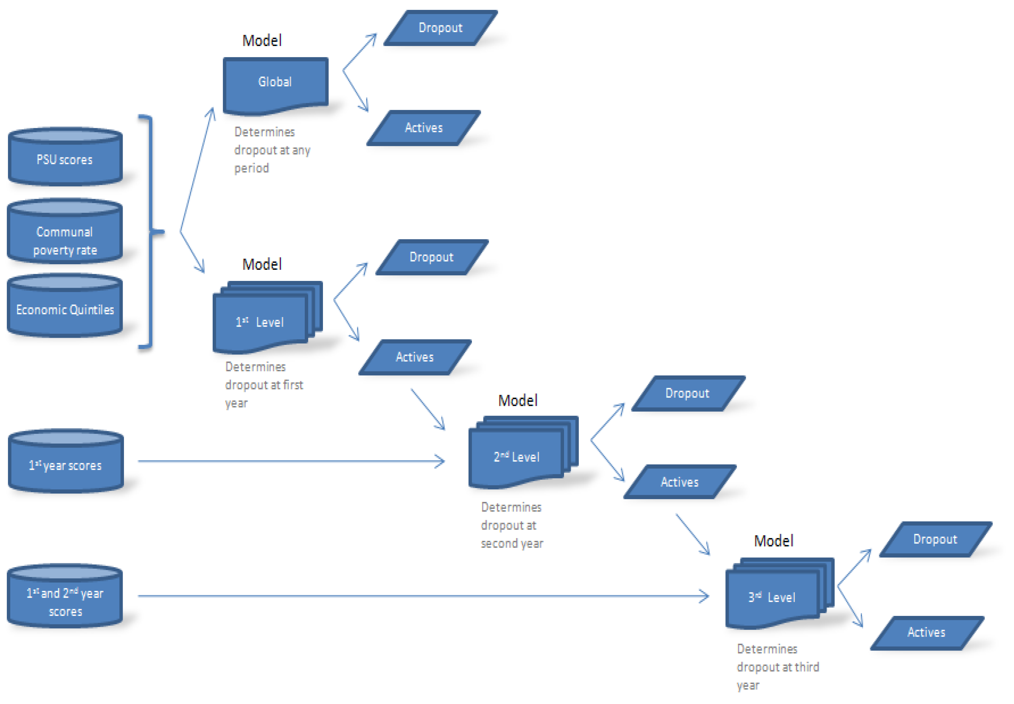
1.4. Models and Description of Sections
2. Methodology
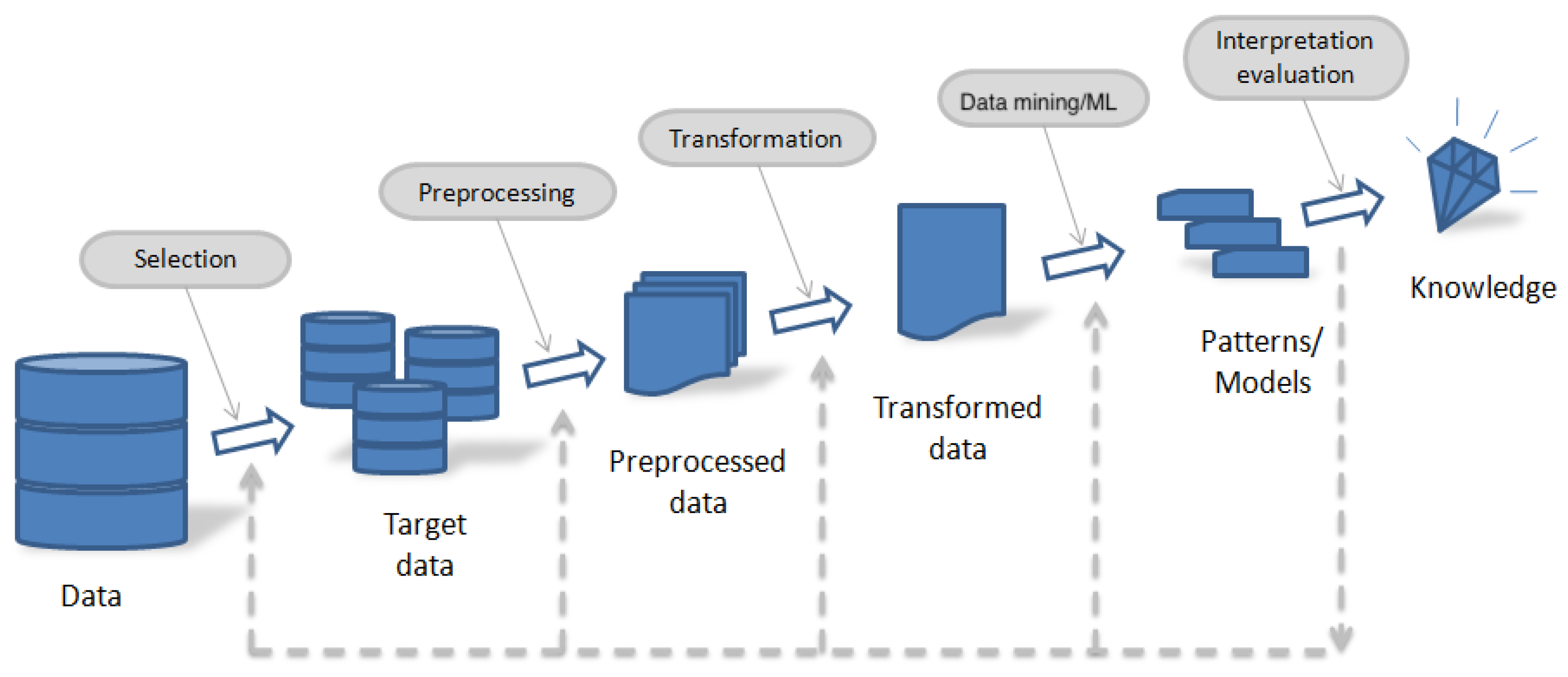
2.1. Contextualization
- (i)
- Data selection,
- (ii)
- Preprocessing,
- (iii)
- Transformation,
- (iv)
- Data mining/ML algorithms, and
- (v)
- Interpretation/evaluation [43].
2.2. Data Selection
2.3. Preprocessing and Transformation
2.4. Data Mining/ML Algorithms
2.5. Data Mining/ML Algorithms’ Performance
2.6. Interpretation and Evaluation
3. Case Study
3.1. ML Algorithms and Computer Configurations
| Algorithm 1: Methodology proposed to predict student retention/dropout in HE institutions similar to the Chilean case. |
|
3.2. Data Selection
3.3. Preprocessing, Transformation of Data, and Initial Results
3.4. Performance Evaluation of Predictive Models
3.5. Interpretation and Evaluation
4. Conclusions, Results, Limitations, Knowledge Discovery, and Future Work
- (a)
- Implement a new information system that enables different databases to coexist for the quick acquisition of necessary information. Data warehouse compilation requires extensive time to extract the relevant data from university records.
- (b)
- Establish a data-monitoring plan to track the enrollment of all students for further analysis and decision-making.
- (c)
- Create a model for predicting students at risk of dropout at different levels of study.
- (d)
- Employ a welcome plan for at-risk students who are identified by the predictive model, in order to assist in improving academic results.
- (e)
- Offer a support program at all grade levels for identifying at-risk students.
- (f)
- In order to increase the innovation of future works, a voting scheme of the machine learning algorithms used can be proposed or the explainability of an examined classifier may be promoted. Voting is an ensemble learning algorithm that, for example in regression, performs a prediction from the mean of several other regressions. In particular, majority voting is used when every model carries out a prediction (votes) for each test instance and the final output prediction obtains more than half of the votes. If none of the predictions reach this majority of votes, the ensemble algorithm is not able to perform a stable prediction for such an instance.
Author Contributions
Funding
Data Availability Statement
Acknowledgments
Conflicts of Interest
Appendix A. Friedman Test Results and Post-Hoc Analysis

| Friedman Test (Significance Level of 0.05) | |||
|---|---|---|---|
| Statistic | p-value | Result | |
| 360.428080 | 0.00000 | H0 is rejected | |
| Friedman Value | Algorithm | Ranking | |
| 3.44875 | SVM | 1 | |
| 3.45125 | RF | 2 | |
| 3.48317 | LR | 3 | |
| 3.49475 | DT | 4 | |
| 3.51025 | NB | 5 | |
| 3.61317 | KNN | 6 | |
| Post-Hoc Analysis (Significance Level of 0.05) | |||
| Comparison | Statistic | p-value | Result |
| KNN vs. SVM | 4.16872 | 0.00046 | H0 is rejected |
| KNN vs. RF | 4.10534 | 0.00057 | H0 is rejected |
| KNN vs. LR | 3.29610 | 0.01274 | H0 is rejected |
| KNN vs. DT | 3.00241 | 0.03214 | H0 is rejected |
| KNN vs. NB | 2.60941 | 0.09977 | H0 is accepted |
| NB vs. SVM | 1.55931 | 1.00000 | H0 is accepted |
| NB vs. RF | 1.49592 | 1.00000 | H0 is accepted |
| DT vs. SVM | 1.16631 | 1.00000 | H0 is accepted |
| RF vs. DT | 1.10293 | 1.00000 | H0 is accepted |
| LR vs. SVM | 0.87262 | 1.00000 | H0 is accepted |
| RF vs. LR | 0.80924 | 1.00000 | H0 is accepted |
| NB vs. LR | 0.68669 | 1.00000 | H0 is accepted |
| NB vs. DT | 0.39300 | 1.00000 | H0 is accepted |
| LR vs. DT | 0.29369 | 1.00000 | H0 is accepted |
| RF vs. SVM | 0.06339 | 1.00000 | H0 is accepted |
| Friedman Test (Significance Level of 0.05) | |||
|---|---|---|---|
| Statistic | p-value | Result | |
| 361.260066 | 0.00000 | H0 is rejected | |
| Friedman Value | Algorithm | Ranking | |
| 3.42083 | RF | 1 | |
| 3.44033 | DT | 2 | |
| 3.47883 | SVR | 3 | |
| 3.48183 | LR | 4 | |
| 3.56733 | NB | 5 | |
| 3.61133 | KNN | 6 | |
| Post-Hoc Analysis (Significance Level of 0.05) | |||
| Comparison | Statistic | p-value | Result |
| KNN vs. RF | 4.83006 | 0.00002 | H0 is rejected |
| KNN vs. DT | 4.33564 | 0.00020 | H0 is rejected |
| NB vs. RF | 3.71445 | 0.00265 | H0 is rejected |
| KNN vs. SVR | 3.35949 | 0.00937 | H0 is rejected |
| KNN vs. LR | 3.28342 | 0.01128 | H0 is rejected |
| NB vs. DT | 3.22004 | 0.01282 | H0 is rejected |
| NB vs. SVR | 2.24388 | 0.22356 | H0 is accepted |
| NB vs. LR | 2.16782 | 0.24138 | H0 is accepted |
| RF vs. LR | 1.54663 | 0.85366 | H0 is accepted |
| RF vs. SVR | 1.47057 | 0.85366 | H0 is accepted |
| KNN vs. NB | 1.11560 | 1.00000 | H0 is accepted |
| LR vs. DT | 1.05222 | 1.00000 | H0 is accepted |
| DT vs. SVR | 0.97615 | 1.00000 | H0 is accepted |
| RF vs. DT | 0.49442 | 1.00000 | H0 is accepted |
| LR vs. SVR | 0.07606 | 1.00000 | H0 is accepted |
| Friedman Test (Significance Level of 0.05) | |||
|---|---|---|---|
| Statistic | p-value | Result | |
| 362.345869 | 0.00000 | H0 is rejected | |
| Friedman Value | Algorithm | Ranking | |
| 3.41825 | RF | 1 | |
| 3.45425 | SVM | 2 | |
| 3.45675 | DT | 3 | |
| 3.48625 | LR | 4 | |
| 3.49425 | KNN | 5 | |
| 3.69075 | NB | 6 | |
| Post-Hoc Analysis (Significance Level of 0.05) | |||
| Comparison | Statistic | p-value | Result |
| NB vs. RF | 6.90914 | 0.00000 | H0 is rejected |
| SVM vs. NB | 5.99637 | 0.00000 | H0 is rejected |
| NB vs. DT | 5.93298 | 0.00000 | H0 is rejected |
| NB vs. LR | 5.18502 | 0.00000 | H0 is rejected |
| KNN vs. NB | 4.98218 | 0.00001 | H0 is rejected |
| KNN vs. RF | 1.92695 | 0.53986 | H0 is accepted |
| RF vs. LR | 1.72411 | 0.76218 | H0 is accepted |
| KNN vs. SVM | 1.01419 | 1.00000 | H0 is accepted |
| RF vs. DT | 0.97615 | 1.00000 | H0 is accepted |
| KNN vs. DT | 0.95080 | 1.00000 | H0 is accepted |
| SVM vs. RF | 0.91277 | 1.00000 | H0 is accepted |
| SVM vs. LR | 0.81135 | 1.00000 | H0 is accepted |
| LR vs. DT | 0.74796 | 1.00000 | H0 is accepted |
| KNN vs. LR | 0.20284 | 1.00000 | H0 is accepted |
| SVM vs. DT | 0.06339 | 1.00000 | H0 is accepted |
| Friedman Test (Significance Level of 0.05) | |||
|---|---|---|---|
| Statistic | p-value | Result | |
| 360.476685 | 0.00000 | H0 is rejected | |
| Friedman Value | Algorithm | Ranking | |
| 3.35866 | DT | 1 | |
| 3.38406 | RF | 2 | |
| 3.43132 | KNN | 3 | |
| 3.45825 | SVM | 4 | |
| 3.60561 | LR | 5 | |
| 3.76270 | NB | 6 | |
| Post-Hoc Analysis (Significance Level of 0.05) | |||
| Comparison | Statistic | Adjusted p-value | Result |
| KNN vs. NB | 8.33467 | 0.00000 | H0 is rejected |
| NB vs. RF | 9.52320 | 0.00000 | H0 is rejected |
| NB vs. DT | 10.16220 | 0.00000 | H0 is rejected |
| SVM vs. NB | 7,65733 | 0.00000 | H0 is rejected |
| LR vs. DT | 6.21106 | 0.00000 | H0 is rejected |
| RF vs. LR | 5.57207 | 0.00000 | H0 is rejected |
| KNN vs. LR | 4.38353 | 0.00011 | H0 is rejected |
| NB vs. LR | 3.95114 | 0.00062 | H0 is rejected |
| SVM vs. LR | 3.70619 | 0.00147 | H0 is rejected |
| SVM vs. DT | 2.50487 | 0.07350 | H0 is accepted |
| SVM vs. RF | 1.86588 | 0.31029 | H0 is accepted |
| KNN vs. DT | 1.82754 | 0.31029 | H0 is accepted |
| KNN vs. RF | 1.18854 | 0.70387 | H0 is accepted |
| KNN vs. SVM | 0.67734 | 0.99638 | H0 is accepted |
| RF vs. DT | 0.63900 | 0.99638 | H0 is accepted |
References
- Berry, M.; Linoff, G. Big Data, Data Mining, and Machine Learning: Value Creation for Business Leaders and Practitioners; Wiley: New York, NY, USA, 1997. [Google Scholar]
- Aykroyd, R.G.; Leiva, V.; Ruggeri, F. Recent developments of control charts, identification of big data sources and future trends of current research. Technol. Forecast. Soc. Chang. 2019, 144, 221–232. [Google Scholar] [CrossRef]
- Fayyad, U.; Piatetsky-Shapiro, G.; Smyth, P. From data mining to knowledge discovery in databases. AI Mag. 1996, 17, 37–54. [Google Scholar]
- Adhikari, A.; Adhikari, J. Advances in Knowledge Discovery in Databases; Springer: New York, NY, USA, 2015. [Google Scholar]
- Tan, P.; Steinbach, M.; Karpatne, A.; Kumar, V. Introduction to Data Mining; Pearson Education: Delhi, India, 2018. [Google Scholar]
- Hastie, T.; Tibshirani, R. The Elements of Statistical Learning: Data Mining, Inference, and Prediction; Springer: New York, NY, USA, 2016. [Google Scholar]
- Delen, D. A comparative analysis of machine learning techniques for student retention management. Decis. Support Syst. 2010, 49, 498–506. [Google Scholar] [CrossRef]
- Delen, D.; Zaim, H.; Kuzey, C.; Zaim, S. A comparative analysis of machine learning systems for measuring the impact of knowledge management practices. Decis. Support Syst. 2013, 54, 1150–1160. [Google Scholar] [CrossRef]
- Gansemer-Topf, A.M.; Schuh, J.H. Institutional selectivity and institutional expenditures: Examining organizational factors that contribute to retention and graduation. Res. High. Educ. 2006, 47, 613–642. [Google Scholar] [CrossRef]
- Hooshyar, D.; Pedaste, M.; Yang, Y. Mining educational data to predict students’ performance through procrastination behavior. Entropy 2020, 22, 12. [Google Scholar] [CrossRef] [PubMed] [Green Version]
- Qu, S.; Li, K.; Wu, B.; Zhang, X.; Zhu, K. Predicting student performance and deficiency in mastering knowledge points in MOOCs using multi-task learning. Entropy 2019, 21, 1216. [Google Scholar] [CrossRef] [Green Version]
- Aguayo, I.; Gómez, G. Evolution in the Number of Enrollments in the Higher Education System, 1983–2010; Technical Report; Chilean Higher Education Information System: Santiago, Chile, 2011. (In Spanish) [Google Scholar]
- SIES. Registered Ration Report in Higher Education in Chile; Technical Report; Chilean Ministry of Education: Santiago, Chile, 2018. (In Spanish) [Google Scholar]
- MINEDUC. Dropout in Higher Education in Chile; Technical Report; Chilean Ministry of Education (MINEDUC): Santiago, Chile, 2012. (In Spanish) [Google Scholar]
- Bakhshinategh, B.; Zaiane, O.R.; Elatia, S.; Ipperciel, D. Educational data mining applications and tasks: A survey of the last 10 years. Educ. Inf. Technol. 2018, 23, 537–553. [Google Scholar] [CrossRef]
- Tinto, V. Dropout of higher education: A theoretical synthesis of recent research. Rev. Educ. Res. 1975, 45, 89–125. [Google Scholar] [CrossRef]
- Himmel, E. Models of analysis of student desertion in higher education. Calid. Educ. 2002, 17, 91–108. (In Spanish) [Google Scholar] [CrossRef] [Green Version]
- Baker, R. Data mining for education. In International Encyclopedia of Education; McGaw, B., Peterson, P., Baker, E., Eds.; Elsevier: Oxford, UK, 2010. [Google Scholar]
- Romero, C.; Ventura, S. Educational data mining: A survey from 1995 to 2005. Expert Syst. Appl. 2007, 33, 135–146. [Google Scholar] [CrossRef]
- Romero, C.; Ventura, S. Data mining in education. Data Min. Knowl. Discov. 2013, 3, 12–27. [Google Scholar] [CrossRef]
- Romero, C.; Ventura, S. Educational data mining: A review of the state of the art. IEE Trans. Syst. Man Cybern. Part Appl. Rev. 2010, 40, 601–618. [Google Scholar] [CrossRef]
- Bousbia, N.; Belamri, I. Which contribution does EDM provide to computer-based learning environments? Stud. Comput. Intell. 2014, 524, 3–28. [Google Scholar]
- Dekker, G.W.; Pechenizkiy, M.; Vleeshouwers, J.M. Predicting students dropout: A case study. In Proceedings of the Second International Working Group on Educational Data Mining, Cordoba, Spain, 1–3 July 2009; pp. 41–50. [Google Scholar]
- Lykourentzou, I.; Giannoukos, I.; Nikolopoulos, V.; Mpardis, G.; Loumos, V. Dropout prediction in e-learning courses through the combination of machine learning techniques. Comput. Educ. 2009, 53, 950–965. [Google Scholar] [CrossRef]
- Nandeshwar, A.; Menzies, T.; Adam, N. Learning patterns of university student retention. Expert Syst. Appl. 2011, 38, 14984–14996. [Google Scholar] [CrossRef]
- Fischer-Angulo, E.S. Model for the Automation of the Process of Determining the Risk of Desertion in University Students. Master’s Thesis, Universidad de Chile, Santiago, Chile, 2012. (In Spanish). [Google Scholar]
- Agrusti, F.; Mezzini, M.; Bonavolontá, G. Deep learning approach for predicting university dropout: A case study at Roma Tre University. J. E-Learn. Knowl. Soc. 2020, 16, 44–54. [Google Scholar]
- Behr, A.; Giese, M.; Theune, K. Early prediction of university dropouts—A random forest approach. J. Econ. Stat. 2020, 240, 743–789. [Google Scholar] [CrossRef]
- Bogard, M.; Helbig, T.; Huff, G.; James, C. A Comparison of Empirical Models for Predicting Student Retention. Working Paper. 2011. Available online: https://www.wku.edu/instres/documents/comparison_of_empirical_models.pdf (accessed on 19 June 2014).
- Del Bonifro, F.; Gabbrielli, M.; Lisanti, G.; Zingaro, S.P. Student Dropout Prediction. In Artificial Intelligence in Education; Bittencourt, I., Cukurova, M., Muldner, K., Luckin, R., Millán, E., Eds.; Springer: Cham, Switzerland, 2020. [Google Scholar]
- Guruler, H.; Istanbullu, A. Modeling student performance in higher education using data mining. In Educational Data Mining; Pena-Ayala, A., Ed.; Springer: Cham, Switzerland, 2014; pp. 105–124. [Google Scholar]
- Iam-On, N.; Boongoen, T. Improved student dropout prediction in Thai University using ensemble of mixed-type data clusterings. Int. J. Mach. Learn. Cybern. 2017, 8, 497–510. [Google Scholar] [CrossRef]
- Lauria, E.; Baron, J.; Devireddy, M.; Sundararaju, V.; Jayaprakash, S. Mining academic data to improve college student retention: An open source perspective. In Proceedings of the 2nd International Conference on Learning Analytics and Knowledge; ACM: New York, NY, USA, 2012; pp. 139–142. [Google Scholar]
- Lázaro, N.; Callejas, Z.; Griol, D. Predicting computer engineering students dropout in cuban higher education with pre-enrollment and early performance data. J. Technol. Sci. Educ. 2020, 10, 241–258. [Google Scholar] [CrossRef]
- Manhães, L.M.; da Cruz, S.M.; Zimbrao, G. Wave: An architecture for predicting dropout in undergraduate courses using edm. In Proceedings of the 29th Annual ACM Symposium on Applied Computing; ACM: New York, NY, USA, 2014; pp. 243–247. [Google Scholar]
- Mellalieu, P. Predicting success, excellence, and retention from students early course performance: Progress results from a data-mining-based decision support system in a first year tertiary education program. In Proceedings of the International Conference of the International Council for Higher Education, Miami, FL, USA, 31 July–4 August 2011. [Google Scholar]
- Raju, D.; Schumacker, R. Exploring student characteristics of retention that lead to graduation in higher education using data mining models. J. Coll. Stud. Retention: Res. Theory Pract. 2015, 16, 563–591. [Google Scholar] [CrossRef]
- Rodríguez-Muñiz, L.J.; Bernardo, A.B.; Esteban, M.; Díaz, I. Dropout and transfer paths: What are the risky profiles when analyzing university persistence with machine learning techniques? PLoS ONE 2019, 14, e0218796. [Google Scholar] [CrossRef]
- Valero, S.; Salvador, A.; García, M. Data mining: Prediction of school desertion using the algorithm of decision trees and the algorithm of the nearest k neighbors. Ene 2005, 779, 33. (In Spanish) [Google Scholar]
- Yadav, S.; Bharadwaj, B.; Pal, S. Mining education data to predict students retention: A comparative study. Int. J. Comput. Sci. Inf. Secur. 2012, 10, 113–117. [Google Scholar]
- Yu, C.; DiGangi, S.; Jannasch-Pennell, A.; Kaprolet, C. A data mining approach for identifying predictors of student retention from sophomore to junior year. J. Data Sci. 2010, 8, 307–325. [Google Scholar]
- Gutiérrez-Salazar, H. Proposed Extension of Kohonen Self-Organized Maps Using Fuzzy Logic to Be Used in Data Mining, a Practical Case. Master’s Thesis, Universidad Católica del Maule, Talca, Chile, 2010. (In Spanish). [Google Scholar]
- Debuse, J.; de la Iglesia, B.; Howard, C.; Rayward-Smith, V. Building the KDD Roadmap. In Industrial Knowledge Management; Roy, R., Ed.; Springer: London, UK, 2001. [Google Scholar]
- Olson, D.L.; Delen, D. Advanced Data Mining Techniques; Springer: New York, NY, USA, 2008. [Google Scholar]
- Yang, Y.; Pedersen, J. A comparative study on feature selection in text categorization. In Proceedings of the Fourteenth International Conference on Machine Learning, San Francisco, CA, USA, 8–12 July 1997; pp. 412–420. [Google Scholar]
- Mduma, N.; Kalegele, K.; Machuve, D. Machine learning approach for reducing students dropout rates. Int. J. Adv. Comput. Res. 2019, 9, 156–169. [Google Scholar] [CrossRef]
- Fawcett, T. An introduction to ROC analysis. Pattern Recognit. Lett. 2006, 27, 861–874. [Google Scholar] [CrossRef]
- Daniel, W.W. Applied Nonparametric Statistics; PWS-Kent Pulisher: Boston, MA, USA, 1990. [Google Scholar]
- Rodriguez-Fdez, I.; Canosa, A.; Mucientes, M.; Bugarin, A. STAC: A web platform for the comparison of algorithms using statistical tests. In Proceedings of the 2015 IEEE International Conference on Fuzzy Systems (FUZZ-IEEE), Istanbul, Turkey, 2–5 August 2015. [Google Scholar]
- Social Observatory. Incidence of Poverty at the Community Level, According to Estimation Methodology for Small Areas, Chile 2009 and 2011; Technical Report; Ministry of Social Development: Santiago, Chile, 2013. (In Spanish) [Google Scholar]
- Arrau, F.; Loiseau, V. Dropout in Higher Education in Chile; Technical Report; Library of the National Congress of Chile: Valparaiso, Chile, 2003. (In Spanish) [Google Scholar]
- Chawla, N.V.; Bowyer, K.W.; Hall, L.O.; Kegelmeyer, W.P. Smote: Synthetic minority over-sampling technique. J. Artif. Intell. Res. 2002, 16, 321–357. [Google Scholar] [CrossRef]


| Abbreviations/Acronyms | Notations/Symbols | ||
|---|---|---|---|
| ANN | artificial neural networks | ∼ | distributed as |
| CLU | clustering | k | number of nearest neighbors |
| CP | community poverty index | n | sample size |
| DT | decision trees | log-odd | |
| EDM | educational data mining | odd | |
| EM | ensemble models | regression coefficients | |
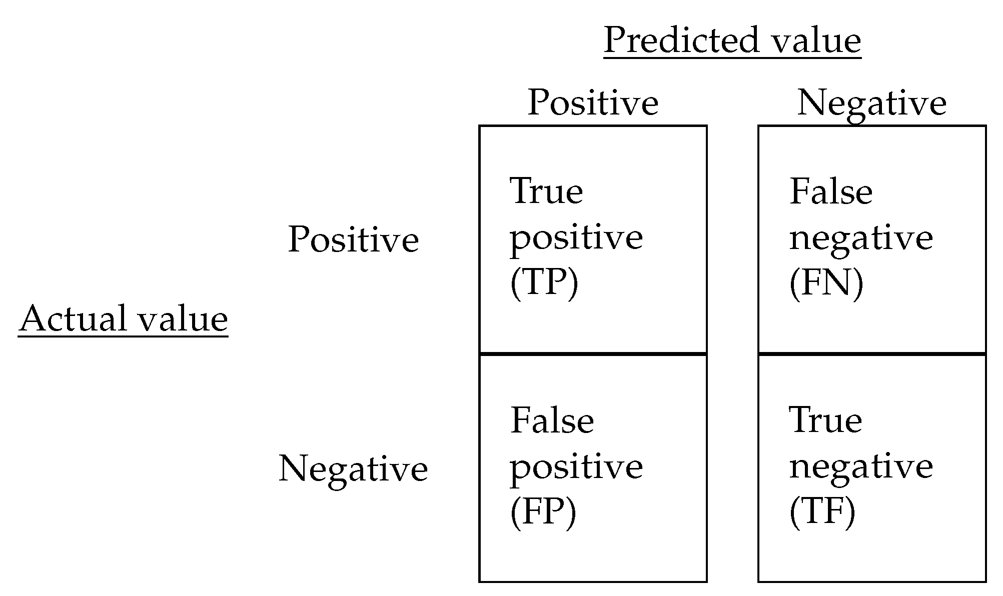
| FN | false negative | X | independent variable or feature |
| FP | false positive | Y | dependent variable or response |
| HE | higher education | probability function of LR | |
| IG | information gain | ||
| KNN | k-nearest neighbors | ||
| LR | logistic regression | probability Y given | |
| ML | machine learning | Bayes conditional probability | |
| NB | naive Bayes | vector of independent variables | |
| NEM | secondary educational score | instances | |
| (notas enseñanza media) | c | number of classes | |
| PSU | university selection test | norm of a point x | |
| (prueba selección universitaria) | s | number of folds in cross-validation | |
| RAM | random access memory | normal vector to the hyperplane | |
| RF | random forest | TP/(TP + FP) | precision |
| SVM | support vector machines | -statistic | |
| TF | true negative | % of agreement classifier/ground truth | |
| TP | true positive | agreement chance | |
| UCM | Catholic University of Maule | Friedman statistic | |
| (Universidad Católica del Maule) | data matrix | ||
| SMOTE | synthetic minority | rank matrix | |
| over-sampling technique | rank average of column j | ||
| KDD | knowledge discovery | p-value | |
| in databases | chi-squared distribution | ||
| with c degrees of freedom | |||
| Reference | Instances | Technique(s) | Confusion Matrix | Accuracy | Institution | Country |
|---|---|---|---|---|---|---|
| [7,8] | 16,066 | ANN, DT, SVM, LR | Yes | 87.23% | Oklahoma State | |
| University | USA | |||||
| [23] | 713 | DT, NB, LR, EM, RF | Yes | 80% | Eindhoven University | |
| of Technology | Netherlands | |||||
| [24] | N/A | ANN, SVM, EM | No | N/A | National Technical | |
| University of Athens | Greece | |||||
| [25] | 8025 | DT, NB | Yes | 79% | Kent State | |
| University | USA | |||||
| [26] | 452 | ANN, DT, KNN | Yes | N/A | University | |
| of Chile | Chile | |||||
| [27] | 6078 | NN, NB | Yes | N/A | Roma Tre | |
| University | Italy | |||||
| [28] | 17,910 | RF, DT | Yes | N/A | University | |
| of Duisburg | Germany | |||||
| [29] | N/A | LR, DT, ANN, EM | No | N/A | N/A | |
| N/A | USA | |||||
| [30] | 1500 | CLU, SVM, RF | No | N/A | University | |
| of Bologna | Italy | |||||
| [31] | 6470 | DT | No | 87% | Mugla Sitki | |
| Kocman University | Turkey | |||||
| [32] | 811 | EM, NB, KNN, ANN | No | N/A | Mae Fah | |
| Luang University | Thailand | |||||
| [33] | 3877 | LR, SVM, DT | No | N/A | Purdue | |
| University | USA | |||||
| [34] | 456 | ANN, DT | No | N/A | University of | |
| Computer Science | Cuba | |||||
| [35] | 1359 | NB, SVM | Yes | 87% | Federal University | |
| of Rio de Janeiro | Brazil | |||||
| [36] | N/A | N/A | No | 61% | Unitec Institute | New |
| of Technology | Zealand | |||||
| [37] | 22,099 | LR, DT, ANN | No | N/A | several | |
| universities | USA | |||||
| [38] | 1055 | C45, RF, CART, SVM | No | 86.6% | University | |
| of Oviedo | Spain | |||||
| [39] | 6500 | DT, KNN | No | 98.98% | Technical University | |
| of Izúcar | Mexico | |||||
| [40] | N/A | DT | Yes | N/A | N/A | |
| N/A | India | |||||
| [41] | 6690 | ANN, LR, DT | No | 76.95% | Arizona State | |
| University | USA |
| Attributes | Features |
|---|---|
| Demographic background | Name, age, gender. |
| Geographic origin | Place of origin, province. |
| Socioeconomic index | CP index. |
| School performance | High school grades, secondary educational score (NEM), PSU score. |
| University performance | Number of approved courses, failed courses, approved credits, failed credits. |
| Financial indicators | Economic quintile, family income. |
| Others | Readmissions, program, application preference, selected/waiting list, health insurance. |
| Attributes | ||
|---|---|---|
| Age Application preference Approved credits 1th semester Approved credits 2nd semester Approved credits 3rd semester Approved credits 4th semester Approved courses 1th semester Approved courses 2nd semester Approved courses 3rd semester Approved courses 4th semester CP index Dependent group Educational area Entered credits 1th semester | Entered credits 2nd semester Entered credits 3rd semester Entered credits 4th semester Family income Gender Graduate/non-graduate Health insurance Marks 1th semester Marks 2nd semester Marks 3rd semester Marks 4th semester NEM Program Province | PSU averaged score in language/maths PSU score of language PSU score of maths PSU score of specific topic PSU weighted score Quintile Readmissions Registered courses 1th semester Registered courses 2nd semester Registered courses 3rd semester Registered courses 4th semester School Selected/waiting list |
| Global | First Level | Second Level | Third Level | |||||
|---|---|---|---|---|---|---|---|---|
| Rank | IG | Variable | IG | Variable | IG | Variable | IG | Variable |
| 1 | 0.430 | NEM | 0.511 | NEM | 0.357 | NEM | 0.098 | Marks 3rd semester |
| 2 | 0.385 | CP index | 0.468 | CP index | 0.220 | CP index | 0.087 | Marks 4th semester |
| 3 | 0.209 | Program | 0.286 | School | 0.211 | School | 0.084 | Approved courses 3rd semester |
| 4 | 0.204 | School | 0.190 | Program | 0.211 | Approved courses 2nd semester | 0.083 | Approved courses 2nd semester |
| 5 | 0.105 | PSU specific topic | 0.112 | PSU specific topic | 0.195 | Approved credits 2nd semester | 0.074 | School |
| 6 | 0.068 | Quintile | 0.110 | PSU language | 0.183 | Approved credits 1st semester | 0.069 | Marks 1st semester |
| 7 | 0.059 | Gender | 0.098 | Quintile | 0.176 | Approved courses 1st semester | 0.067 | Approved courses 4th semester |
| 8 | 0.051 | Family income | 0.056 | Age | 0.163 | Marks 1st semester | 0.066 | Approved courses 1st semester |
| 9 | 0.041 | Age | 0.053 | Educational area | 0.149 | Program | 0.063 | Marks 2nd semester |
| 10 | 0.037 | Educational area | 0.047 | PSU weighted score | 0.141 | Marks 2nd semester | 0.059 | Approved credits 1st semester |
| 11 | 0.034 | PSU language | 0.043 | Graduate/non-graduate | 0.130 | Entered credits 2nd semester | 0.059 | Entered credits 2nd semester |
| 12 | 0.030 | Province | 0.037 | Family income | 0.103 | Entered credits 1st semester | 0.056 | Approved credits 2nd semester |
| 13 | 0.027 | Application preference | 0.034 | Province | 0.079 | Registered courses 2nd semester | 0.051 | Approved credits 4th semester |
| 14 | 0.026 | Health insurance | 0.033 | Gender | 0.058 | Gender | 0.049 | Entered credits 3rd semester |
| 15 | 0.025 | Readmissions | 0.030 | PSU math | 0.038 | Registered courses 1st semester | 0.049 | Program |
| 16 | 0.025 | PSU weighted score | 0.029 | Readmissions | 0.032 | Province | 0.048 | Entered credits 4th semester |
| 17 | 0.019 | PSU math | 0.028 | Health insurance | 0.030 | Family income | 0.044 | Approved credits 3rd semester |
| 18 | 0.015 | Graduate/non-graduate | 0.025 | PSU language/math | 0.029 | Quintile | 0.042 | Registered courses 1st semester |
| 19 | 0.014 | PSU language/math | 0.022 | Application preference | 0.025 | Age | 0.030 | Registered courses 3rd semester |
| 20 | 0.001 | Dependent group | 0.001 | Dependent group | 0.024 | Educational area | 0.030 | Registered courses 4th semester |
| ML Algorithm | Accuracy | Precision | TP Rate | FP Rate | F-Measure | RMSE | -Statistic |
|---|---|---|---|---|---|---|---|
| DT | 82.75% | 0.840 | 0.973 | 0.806 | 0.902 | 0.365 | 0.227 |
| KNN | 81.36% | 0.822 | 0.984 | 0.929 | 0.896 | 0.390 | 0.082 |
| LR | 82.42% | 0.849 | 0.954 | 0.739 | 0.898 | 0.373 | 0.271 |
| NB | 79.63% | 0.860 | 0.894 | 0.631 | 0.877 | 0.387 | 0.283 |
| RF | 81.82% | 0.829 | 0.979 | 0.879 | 0.897 | 0.370 | 0.143 |
| SVM | 81.67% | 0.828 | 0.977 | 0.881 | 0.897 | 0.428 | 0.138 |
| Algorithm | Accuracy | Precision | TP Rate | FP Rate | F-Measure | RMSE | -Statistic | Friedman Value (Ranking) |
|---|---|---|---|---|---|---|---|---|
| DT | 82.19% | 0.814 | 0.837 | 0.194 | 0.825 | 0.368 | 0.644 | 3.49475 (4) |
| KNN | 83.93% | 0.859 | 0.814 | 0.135 | 0.836 | 0.363 | 0.679 | 3.61317 (6) |
| LR | 83.45% | 0.825 | 0.851 | 0.182 | 0.838 | 0.351 | 0.669 | 3.48317 (3) |
| NB | 79.14% | 0.791 | 0.796 | 0.213 | 0.793 | 0.399 | 0.583 | 3.51025 (5) |
| RF | 88.43% | 0.860 | 0.920 | 0.151 | 0.889 | 0.301 | 0.769 | 3.45125 (1) |
| SVM | 83.97% | 0.822 | 0.869 | 0.190 | 0.845 | 0.400 | 0.679 | 3.44875 (1) |
| Algorithm | Accuracy | Precision | TP Rate | FP Rate | F-Measure | RMSE | -Statistic | Friedman Value (Ranking) |
|---|---|---|---|---|---|---|---|---|
| DT | 89.21% | 0.888 | 0.933 | 0.166 | 0.910 | 0.294 | 0.775 | 3.44033 (1) |
| KNN | 89.43% | 0.929 | 0.887 | 0.096 | 0.908 | 0.298 | 0.784 | 3.61133 (6) |
| LR | 87.70% | 0.885 | 0.908 | 0.166 | 0.896 | 0.309 | 0.745 | 3.48183 (4) |
| NB | 83.95% | 0.869 | 0.854 | 0.181 | 0.862 | 0.349 | 0.671 | 3.56733 (5) |
| RF | 93.65% | 0.921 | 0.976 | 0.119 | 0.947 | 0.238 | 0.868 | 3.42083 (1) |
| SVM | 88.30% | 0.889 | 0.914 | 0.160 | 0.901 | 0.342 | 0.758 | 3.47883 (3) |
| ML Algorithm | Accuracy | Precision | TP Rate | FP Rate | F-Measure | RMSE | -Statistic | Friedman Value (Ranking) |
|---|---|---|---|---|---|---|---|---|
| DT | 91.06% | 0.938 | 0.954 | 0.288 | 0.946 | 0.278 | 0.687 | 3.45675 (3) |
| KNN | 94.41% | 0.965 | 0.967 | 0.161 | 0.966 | 0.222 | 0.809 | 3.49425 (5) |
| LR | 93.57% | 0.958 | 0.964 | 0.193 | 0.961 | 0.232 | 0.779 | 3.48625 (4) |
| NB | 86.69% | 0.954 | 0.880 | 0.194 | 0.916 | 0.347 | 0.603 | 3.69075 (6) |
| RF | 95.76% | 0.959 | 0.99 | 0.196 | 0.975 | 0.193 | 0.847 | 3.41825 (1) |
| SVM | 94.40% | 0.958 | 0.975 | 0.196 | 0.966 | 0.237 | 0.804 | 3.45425 (2) |
| ML Algorithm | Accuracy | Precision | TP Rate | FP Rate | F-Measure | RMSE | -Statistic | Friedman Value (Ranking) |
|---|---|---|---|---|---|---|---|---|
| DT | 94.99% | 0.955 | 0.993 | 0.739 | 0.974 | 0.208 | 0.360 | 3.35866 (1) |
| KNN | 96.90% | 0.977 | 0.990 | 0.371 | 0.984 | 0.168 | 0.689 | 3.43132 (3) |
| LR | 90.58% | 0.973 | 0.926 | 0.414 | 0.949 | 0.305 | 0.376 | 3.60561 (5) |
| NB | 88.09% | 0.987 | 0.885 | 0.181 | 0.933 | 0.331 | 0.396 | 3.76270 (6) |
| RF | 96.92% | 0.969 | 0.999 | 0.503 | 0.984 | 0.160 | 0.641 | 3.38406 (1) |
| SVM | 96.17% | 0.978 | 0.982 | 0.356 | 0.980 | 0.196 | 0.644 | 3.45825 (4) |
Publisher’s Note: MDPI stays neutral with regard to jurisdictional claims in published maps and institutional affiliations. |
© 2021 by the authors. Licensee MDPI, Basel, Switzerland. This article is an open access article distributed under the terms and conditions of the Creative Commons Attribution (CC BY) license (https://creativecommons.org/licenses/by/4.0/).
Share and Cite
Palacios, C.A.; Reyes-Suárez, J.A.; Bearzotti, L.A.; Leiva, V.; Marchant, C. Knowledge Discovery for Higher Education Student Retention Based on Data Mining: Machine Learning Algorithms and Case Study in Chile. Entropy 2021, 23, 485. https://0-doi-org.brum.beds.ac.uk/10.3390/e23040485
Palacios CA, Reyes-Suárez JA, Bearzotti LA, Leiva V, Marchant C. Knowledge Discovery for Higher Education Student Retention Based on Data Mining: Machine Learning Algorithms and Case Study in Chile. Entropy. 2021; 23(4):485. https://0-doi-org.brum.beds.ac.uk/10.3390/e23040485
Chicago/Turabian StylePalacios, Carlos A., José A. Reyes-Suárez, Lorena A. Bearzotti, Víctor Leiva, and Carolina Marchant. 2021. "Knowledge Discovery for Higher Education Student Retention Based on Data Mining: Machine Learning Algorithms and Case Study in Chile" Entropy 23, no. 4: 485. https://0-doi-org.brum.beds.ac.uk/10.3390/e23040485