
An Improved Stereo Matching Algorithm for Vehicle Speed Measurement System Based on Spatial and Temporal Image Fusion

 , , , ,
Abstract
:1. Introduction
2. Related Works
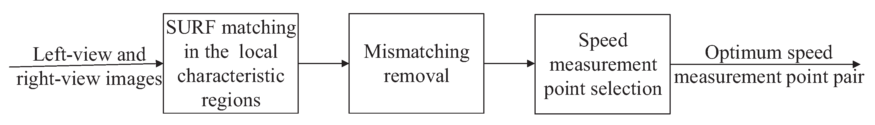
3. Proposed Method
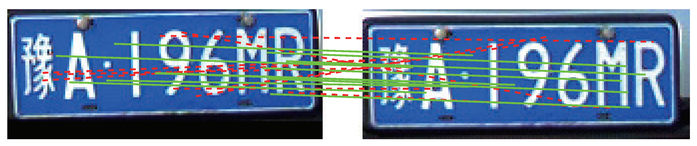
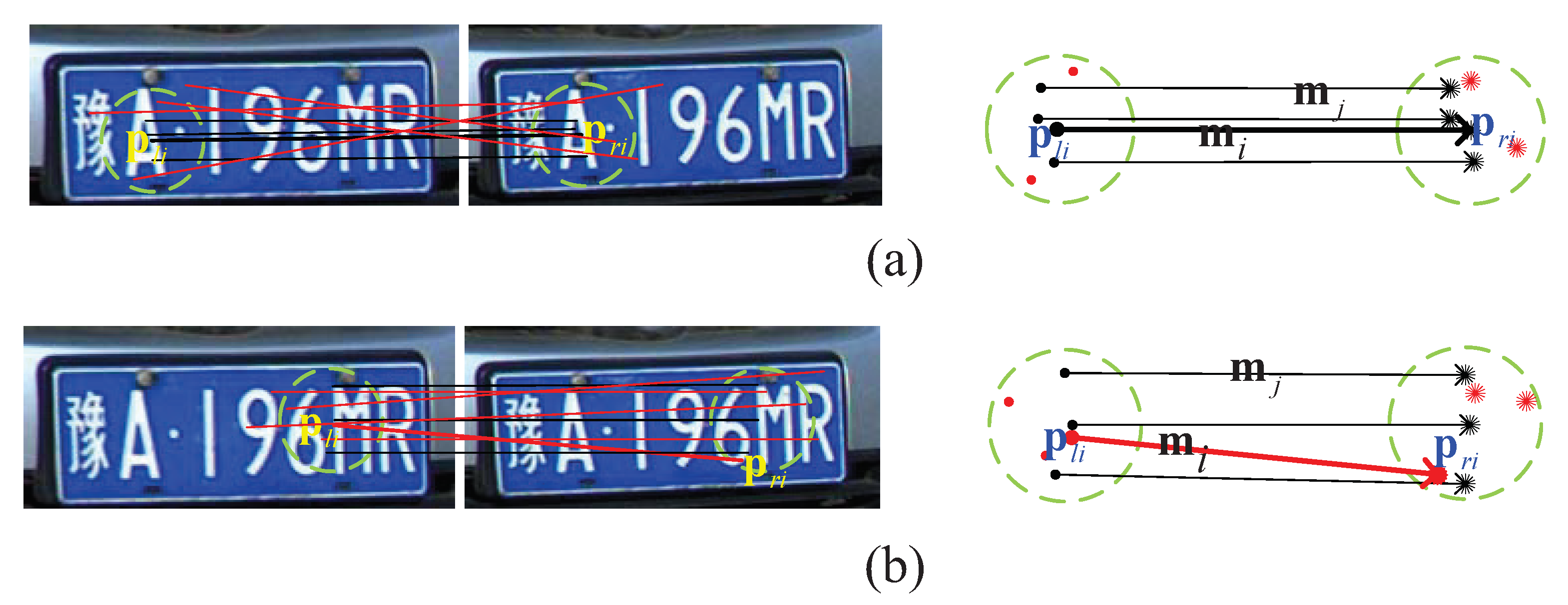
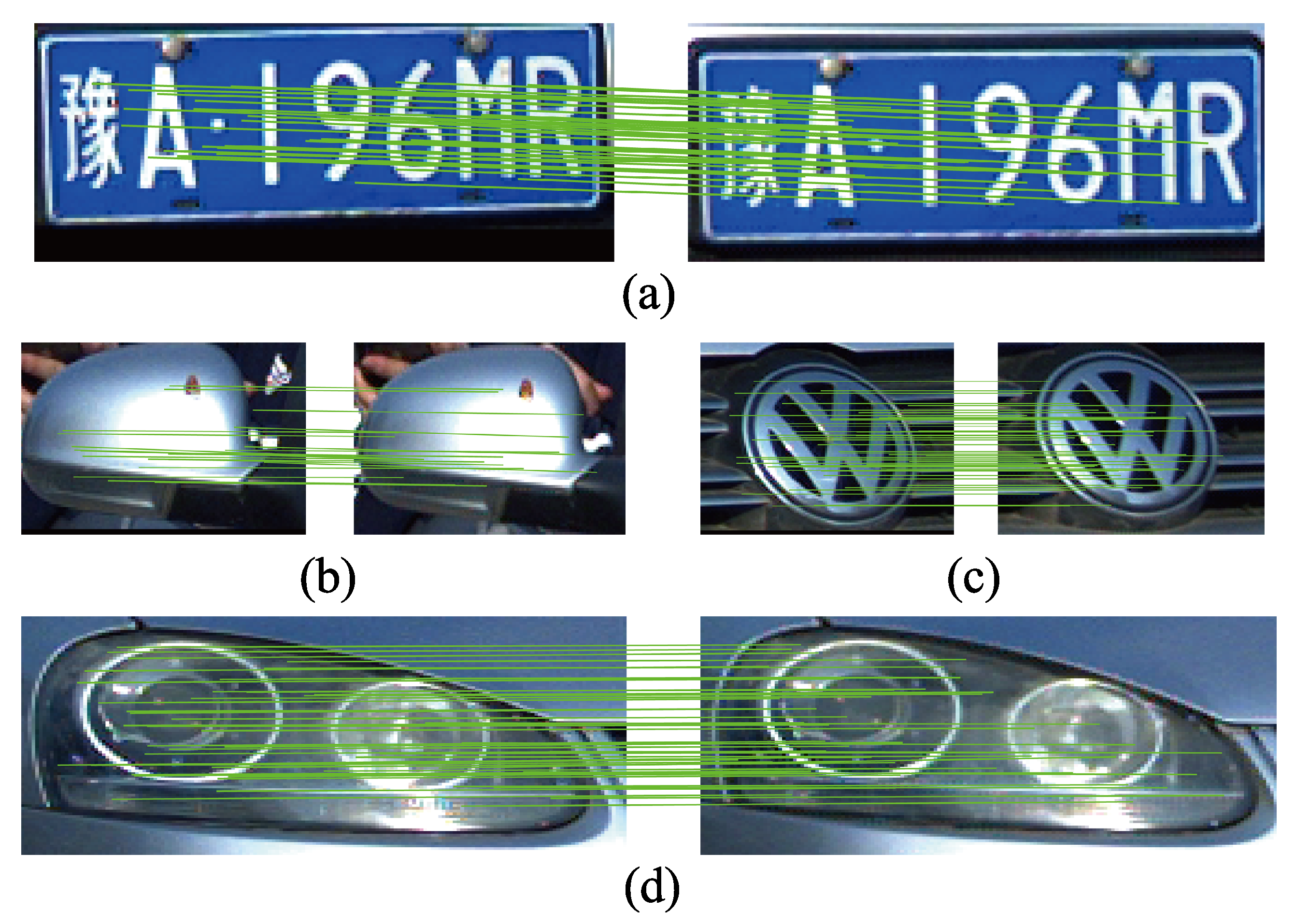
3.1. Mismatching Removal Based on License Plate Specification Constraint (LPSC)
3.2. Mismatching Removal Based on LNCC
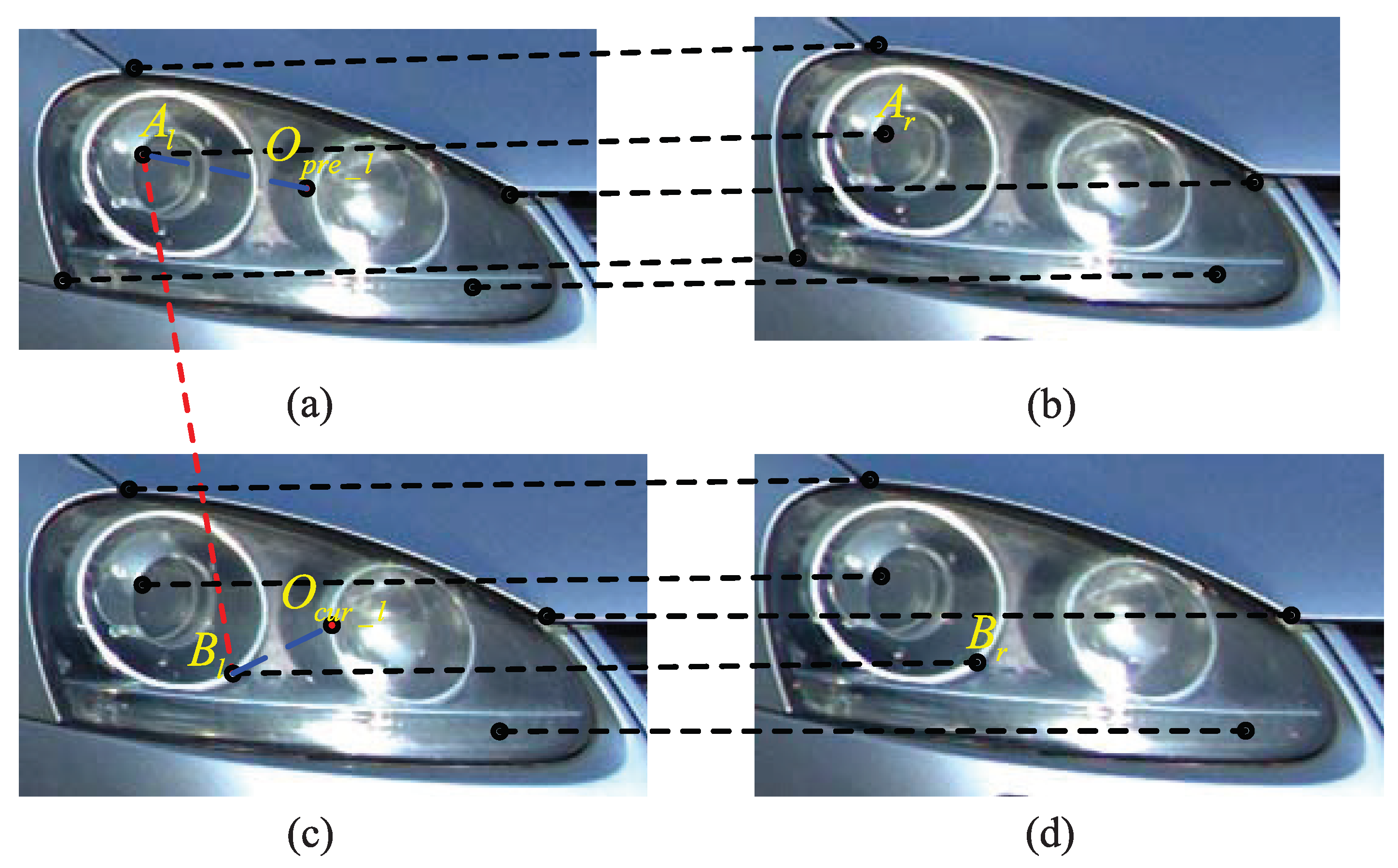
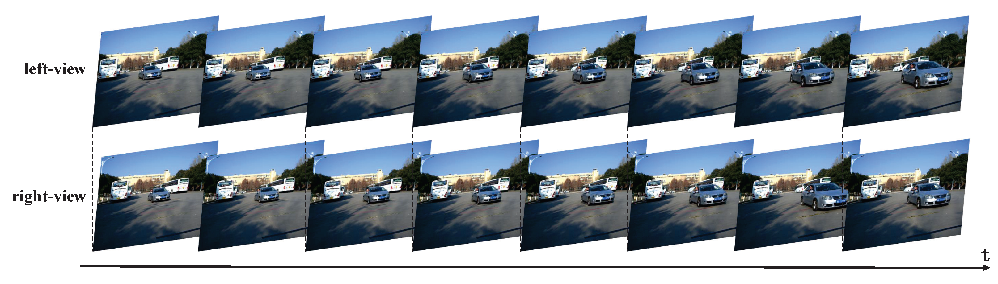
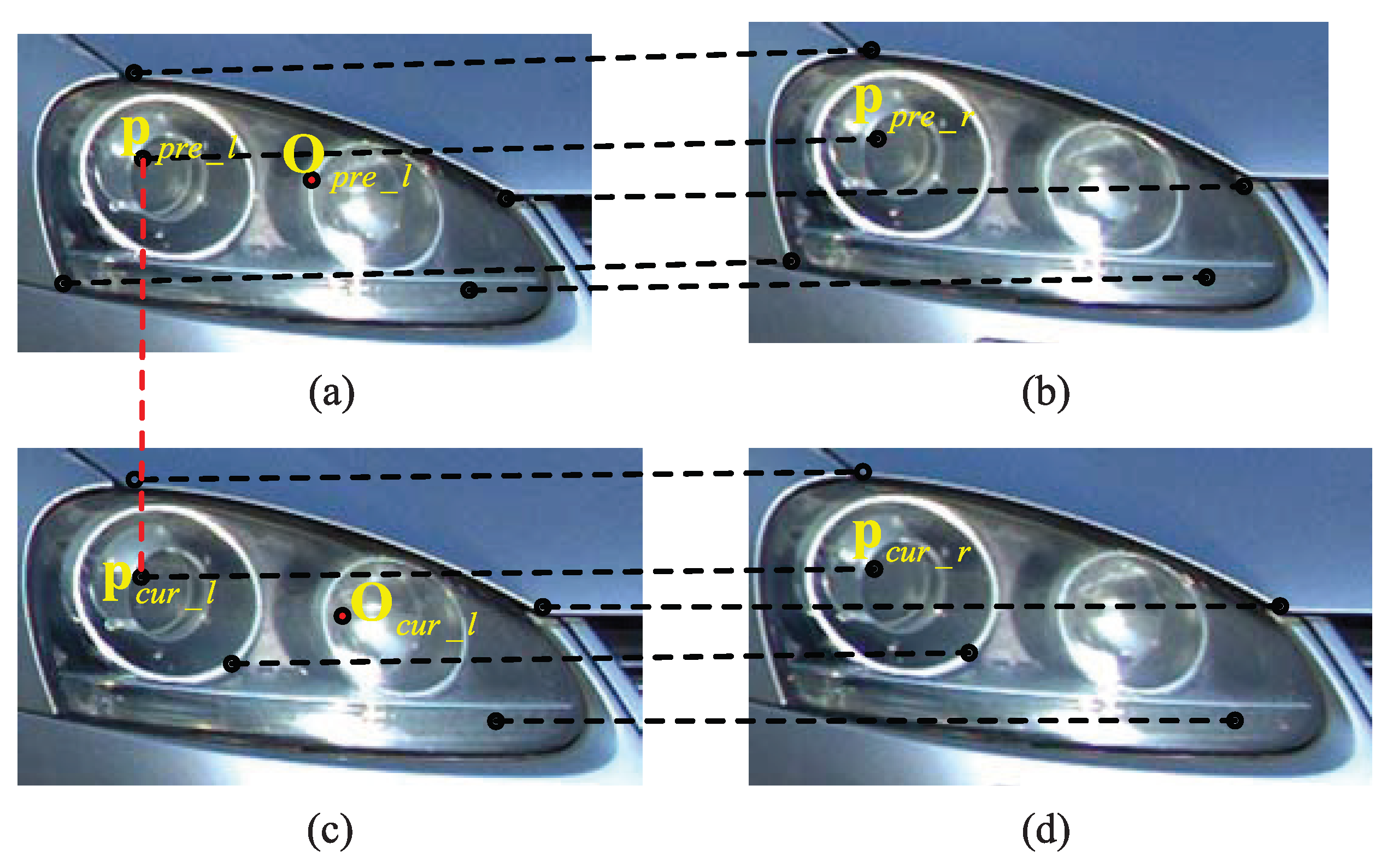
3.3. Speed Measurement Point Selection Based on STIF of Binocular Stereo Video
| Algorithm 1:Optimum speed measurement point selection based on STIF. |
|
4. Experiments
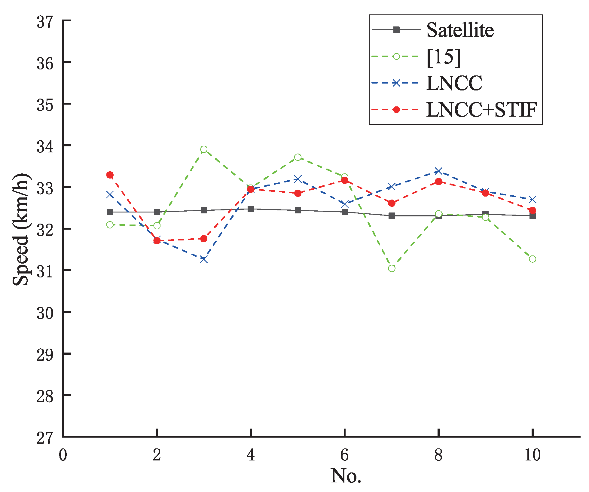
4.1. Speed Measurement Results Based on License Plate
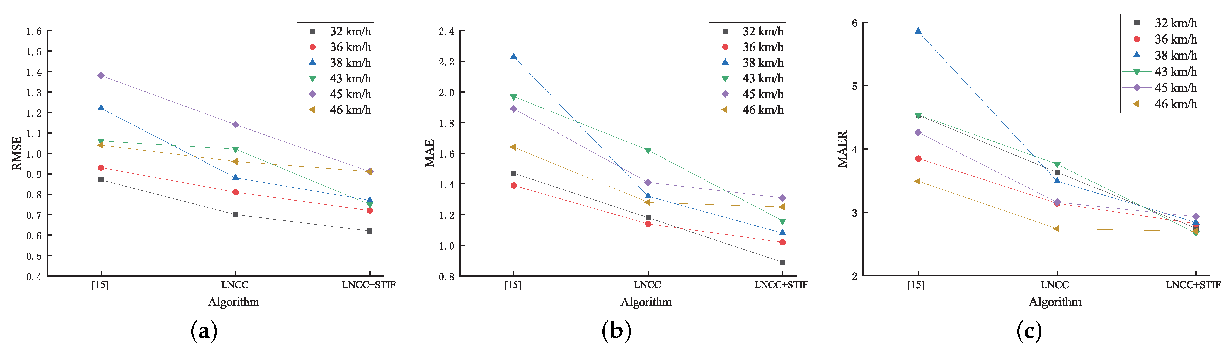
4.2. Speed Measurement Results Based on Other Separate Vehicle Characteristic
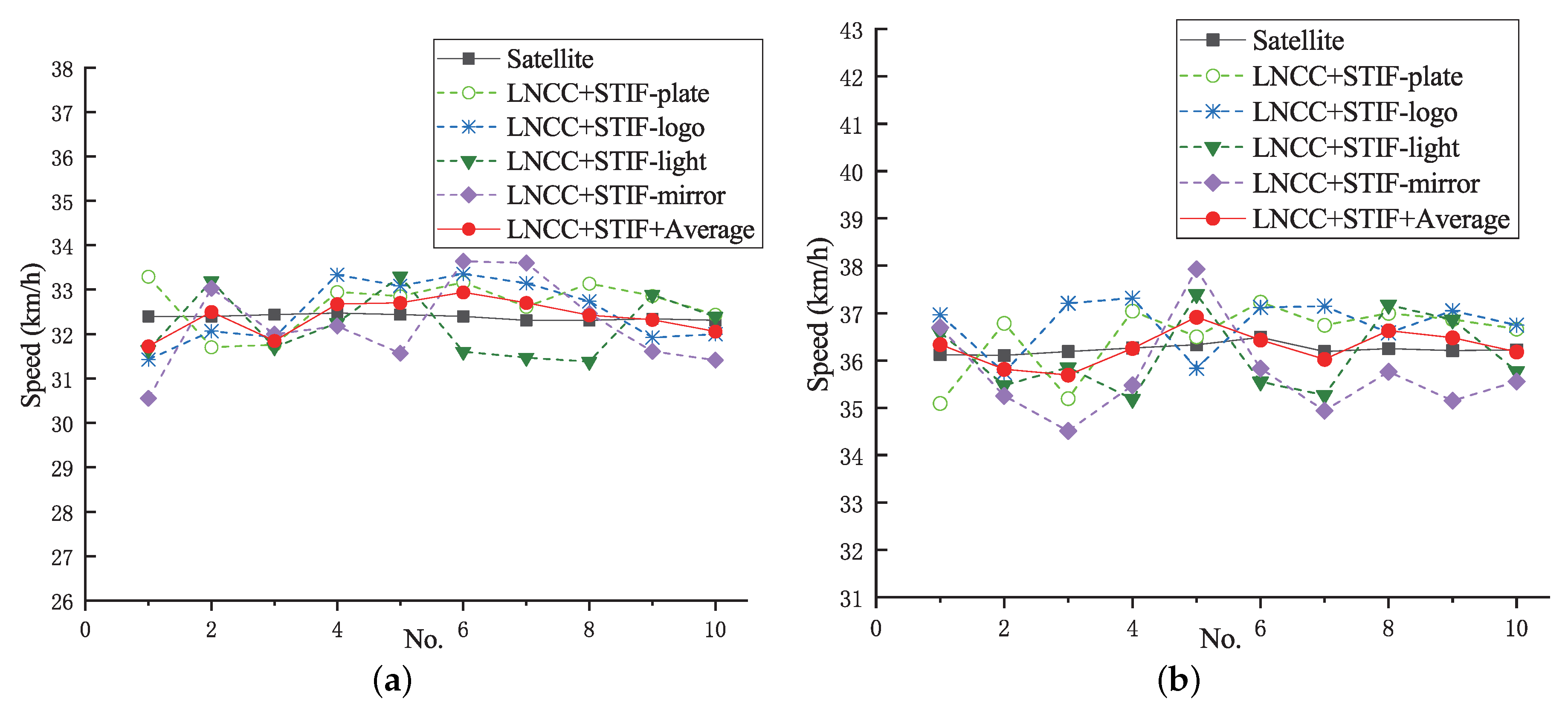
4.3. Speed Measurement Results Based on Multi-Characteristic Combination
5. Conclusions
Author Contributions
Funding
Institutional Review Board Statement
Informed Consent Statement
Data Availability Statement
Conflicts of Interest
References
- Choy, J.L.C.; Wu, J.; Long, C.; Lin, Y.B. Ubiquitous and Low Power Vehicles Speed Monitoring for Intelligent Transport Systems. IEEE Sens. J. 2020, 20, 5656–5665. [Google Scholar] [CrossRef]
- Shin, H.S.; Turchi, D.; He, S.; Tsourdos, A. Behavior Monitoring Using Learning Techniques and Regular-Expressions-Based Pattern Matching. IEEE Trans. Intell. Transp. Syst. 2019, 20, 1289–1302. [Google Scholar] [CrossRef] [Green Version]
- Zhang, C.; Ota, K.; Jia, J.; Dong, M. Breaking the Blockage for Big Data Transmission: Gigabit Road Communication in Autonomous Vehicles. IEEE Commun. Mag. 2018, 56, 152–157. [Google Scholar] [CrossRef] [Green Version]
- Balid, W.; Tafish, H.; Refai, H.H. Intelligent Vehicle Counting and Classification Sensor for Real-Time Traffic Surveillance. IEEE Trans. Intell. Transp. Syst. 2018, 19, 1784–1794. [Google Scholar] [CrossRef]
- Wei, Q.; Yang, B. Adaptable Vehicle Detection and Speed Estimation for Changeable Urban Traffic with Anisotropic Magnetoresistive Sensors. IEEE Sens. J. 2017, 17, 2021–2028. [Google Scholar] [CrossRef]
- Makarov, A. Real-Time Vehicle Speed Estimation Based on License Plate Tracking in Monocular Video Sequences. Sens. Transducers 2016, 197, 78–86. [Google Scholar]
- Ki, Y.K.; Baik, D.K. Model for accurate speed measurement using double-loop detectors. IEEE Trans. Veh. Technol. 2006, 55, 1094–1101. [Google Scholar] [CrossRef]
- Odat, E.; Shamma, J.S.; Claudel, C. Vehicle Classification and Speed Estimation Using Combined Passive Infrared/Ultrasonic Sensors. IEEE Trans. Intell. Transp. Syst. 2018, 19, 1593–1606. [Google Scholar] [CrossRef]
- Quang, V.V.; Linh, N.V.; Thang, V.T.; Phuc, D.V. Vehicle speed estimation using two roadside passive infrared sensors. Int. J. Mod. Phys. B 2020, 34, 2040151. [Google Scholar]
- Jeng, S.L.; Chieng, W.H.; Lu, H.P. Estimating Speed Using a Side-Looking Single-Radar Vehicle Detector. IEEE Trans. Intell. Transp. Syst. 2014, 15, 607–614. [Google Scholar] [CrossRef]
- Luvizon, D.C.; Nassu, B.T.; Minetto, R. A Video-Based System for Vehicle Speed Measurement in Urban Roadways. IEEE Trans. Intell. Transp. Syst. 2017, 18, 1393–1404. [Google Scholar] [CrossRef]
- Famouri, M.; Azimifar, Z.; Wong, A. A Novel Motion Plane-Based Approach to Vehicle Speed Estimation. IEEE Trans. Intell. Transp. Syst. 2019, 20, 1237–1246. [Google Scholar] [CrossRef]
- El Bouziady, A.; Thami, R.O.H.; Ghogho, M.; Bourja, O.; El Fkihi, S. Vehicle speed estimation using extracted SURF features from stereo images. In Proceedings of the 2018 International Conference on Intelligent Systems and Computer Vision (ISCV), Fez, Morocco, 2–4 April 2018; pp. 1–6. [Google Scholar]
- Najman, P.; Zemčík, P. Vehicle Speed Measurement Using Stereo Camera Pair. IEEE Trans. Intell. Transp. Syst. 2020, 1–9. [Google Scholar] [CrossRef]
- Yang, L.; Li, M.; Song, X.; Xiong, Z.; Hou, C.; Qu, B. Vehicle Speed Measurement Based on Binocular Stereovision System. IEEE Access 2019, 7, 106628–106641. [Google Scholar] [CrossRef]
- Liu, Y.; Dominicis, L.D.; Wei, B.; Chen, L.; Martin, R.R. Regularization Based Iterative Point Match Weighting for Accurate Rigid Transformation Estimation. IEEE Trans. Vis. Comput. Graph. 2015, 21, 1058–1071. [Google Scholar] [CrossRef] [PubMed] [Green Version]
- Ma, T.; Ma, J.; Yu, K.; Zhang, J.; Fu, W. Multispectral Remote Sensing Image Matching via Image Transfer by Regularized Conditional Generative Adversarial Networks and Local Feature. IEEE Geosci. Remote Sens. Lett. 2021, 18, 351–355. [Google Scholar] [CrossRef]
- Ghaffari, A.; Fatemizadeh, E. Image Registration Based on Low Rank Matrix: Rank-Regularized SSD. IEEE Trans. Med. Imaging 2018, 37, 138–150. [Google Scholar] [CrossRef] [PubMed]
- Liu, X.; Jing, W.; Zhou, M.; Li, Y. Multi-Scale Feature Fusion for Coal-Rock Recognition Based on Completed Local Binary Pattern and Convolution Neural Network. Entropy 2019, 21, 622. [Google Scholar] [CrossRef] [Green Version]
- Ilyas, A.; Farid, M.S.; Khan, M.H.; Grzegorzek, M. Exploiting Superpixels for Multi-Focus Image Fusion. Entropy 2021, 23, 247. [Google Scholar] [CrossRef] [PubMed]
- Leng, C.; Zhang, H.; Li, B.; Cai, G.; Pei, Z.; He, L. Local Feature Descriptor for Image Matching: A Survey. IEEE Access 2019, 7, 6424–6434. [Google Scholar] [CrossRef]
- Jiang, X.; Ma, J.; Xiao, G.; Shao, Z.; Guo, X. A review of multimodal image matching: Methods and applications. Inf. Fusion 2021, 73, 22–71. [Google Scholar] [CrossRef]
- Ma, J.; Ma, Y.; Li, C. Infrared and visible image fusion methods and applications: A survey. Inf. Fusion 2019, 45, 153–178. [Google Scholar] [CrossRef]
- Reddy, B.; Chatterji, B. An FFT-based technique for translation, rotation, and scale-invariant image registration. IEEE Trans. Image Process. 1996, 5, 1266–1271. [Google Scholar] [CrossRef] [PubMed] [Green Version]
- Rangarajan, A.; Chui, H.; Duncan, J.S. Rigid point feature registration using mutual information. Med. Image Anal. 2000, 3, 425–440. [Google Scholar] [CrossRef]
- Liu, X.; Wang, Z.; Wang, L.; Huang, C.; Luo, X. A Hybrid Rao-NM Algorithm for Image Template Matching. Entropy 2021, 23, 678. [Google Scholar] [CrossRef] [PubMed]
- Ma, J.; Zhao, J.; Tian, J.; Yuille, A.L.; Tu, Z. Robust Point Matching via Vector Field Consensus. IEEE Trans. Image Process. 2014, 23, 1706–1721. [Google Scholar] [CrossRef] [Green Version]
- Ma, J.; Jiang, X.; Fan, A.; Jiang, J.; Yan, J. Image Matching from Handcrafted to Deep Features: A Survey. Int. J. Comput. Vis. 2021, 129, 23–79. [Google Scholar] [CrossRef]
- Xu, X.; Yu, C.; Zhou, J. Robust feature point matching based on geometric consistency and affine invariant spatial constraint. In Proceedings of the 2013 IEEE International Conference on Image Processing, Melbourne, Australia, 15–18 September 2013; pp. 2077–2081. [Google Scholar]
- Kim, J.; Liu, C.; Sha, F.; Grauman, K. Deformable Spatial Pyramid Matching for Fast Dense Correspondences. In Proceedings of the 2013 IEEE Conference on Computer Vision and Pattern Recognition, Portland, OR, USA, 23–28 June 2013; pp. 2307–2314. [Google Scholar]
- Lowe, D.G. Distinctive Image Features from Scale-Invariant Keypoints. Int. J. Comput. Vis. 2004, 60, 91–110. [Google Scholar] [CrossRef]
- Bay, H.; Ess, A.; Tuytelaars, T.; Gool, L.V. Speeded-Up Robust Features (SURF). Comput. Vis. Image Underst. 2008, 110, 346–359. [Google Scholar] [CrossRef]
- Gao, Z.; Wang, L.; Zhou, L. A Probabilistic Approach to Cross-Region Matching-Based Image Retrieval. IEEE Trans. Image Process. 2019, 28, 1191–1204. [Google Scholar] [CrossRef]
- Qu, H.B.; Wang, J.Q.; Li, B.; Yu, M. Probabilistic Model for Robust Affine and Non-Rigid Point Set Matching. IEEE Trans. Pattern Anal. Mach. Intell. 2017, 39, 371–384. [Google Scholar] [CrossRef]
- Wu, Y.; Ma, W.; Gong, M.; Su, L.; Jiao, L. A Novel Point-Matching Algorithm Based on Fast Sample Consensus for Image Registration. IEEE Geosci. Remote Sens. Lett. 2015, 12, 43–47. [Google Scholar] [CrossRef]
- Torr, P.H.S.; Zisserman, A. MLESAC: A New Robust Estimator with Application to Estimating Image Geometry. Comput. Vis. Image Underst. 2000, 78, 138–156. [Google Scholar] [CrossRef] [Green Version]
- Chum, O.; Matas, J. Matching with PROSAC—Progressive sample consensus. In Proceedings of the 2005 IEEE Computer Society Conference on Computer Vision and Pattern Recognition (CVPR’05), San Diego, CA, USA, 20–26 June 2005; Volume 1, pp. 220–226. [Google Scholar]
- Tuytelaars, T.; Mikolajczyk, K. Local Invariant Feature Detectors. Found. Trends Comput. Graph. Vis. 2007, 3, 177–280. [Google Scholar] [CrossRef] [Green Version]
- Gay-Bellile, V.; Bartoli, A.; Sayd, P. Direct Estimation of Nonrigid Registrations with Image-Based Self-Occlusion Reasoning. IEEE Trans. Pattern Anal. Mach. Intell. 2010, 32, 87–104. [Google Scholar] [CrossRef] [PubMed]
- Ma, J.; Qiu, W.; Zhao, J.; Ma, Y.; Yuille, A.L.; Tu, Z. Robust L2E Estimation of Transformation for Non-Rigid Registration. IEEE Trans. Signal Process. 2015, 63, 1115–1129. [Google Scholar] [CrossRef]
- Ma, J.; Zhao, J.; Jiang, J.; Zhou, H.; Guo, X. Locality Preserving Matching. Int. J. Comput. Vis. 2019, 127, 512–531. [Google Scholar] [CrossRef]
- Ma, J.; Jiang, J.; Zhou, H.; Zhao, J.; Guo, X. Guided Locality Preserving Feature Matching for Remote Sensing Image Registration. IEEE Trans. Geosci. Remote Sens. 2018, 56, 4435–4447. [Google Scholar] [CrossRef]
- Jiang, X.; Ma, J.; Jiang, J.; Guo, X. Robust Feature Matching Using Spatial Clustering with Heavy Outliers. IEEE Trans. Image Process. 2020, 29, 736–746. [Google Scholar] [CrossRef]
- Kuppala, K.; Banda, S.; Barige, T.R. An overview of deep learning methods for image registration with focus on feature-based approaches. Int. J. Image Data Fusion 2020, 11, 113–135. [Google Scholar] [CrossRef]
- Ma, J.; Wu, J.; Zhao, J.; Jiang, J.; Zhou, H.; Sheng, Q.Z. Nonrigid Point Set Registration with Robust Transformation Learning Under Manifold Regularization. IEEE Trans. Neural Netw. 2019, 30, 3584–3597. [Google Scholar] [CrossRef] [PubMed]
- Ma, J.; Jiang, X.; Jiang, J.; Zhao, J.; Guo, X. LMR: Learning a Two-Class Classifier for Mismatch Removal. IEEE Trans. Image Process. 2019, 28, 4045–4059. [Google Scholar] [CrossRef] [PubMed]
- Liying, Y.Y. License plates of motor vehicles of the People’s Republic of China. In China National Standard GA 36—2014; Ministry of Public Security, PRC: Beijing, China, 2014. [Google Scholar]
- Cai, Z.; Lan, T.; Zheng, C. Hierarchical MK Splines: Algorithm and Applications to Data Fitting. IEEE Trans. Multimed. 2017, 19, 921–934. [Google Scholar] [CrossRef]
- Wang, X. Research on Target Ranging Technology Based on Binocular Stereo Vision. Master’s Thesis, Zhongyuan University of Technology, Zhengzhou, China, 2018. [Google Scholar]
- Zhang, Z. A flexible new technique for camera calibration. IEEE Trans. Pattern Anal. Mach. Intell. 2000, 22, 1330–1334. [Google Scholar] [CrossRef] [Green Version]
- Yi, P.; Wang, Z.; Jiang, K.; Jiang, J.; Lu, T.; Ma, J. A Progressive Fusion Generative Adversarial Network for Realistic and Consistent Video Super-Resolution. IEEE Trans. Pattern Anal. Mach. Intell. 2020. [Google Scholar] [CrossRef]
- Pan, Z.; Yu, W.; Lei, J.; Ling, N.; Kwong, S. TSAN: Synthesized View Quality Enhancement via Two-Stream Attention Network for 3D-HEVC. IEEE Trans. Circuits Syst. Video Technol. 2021. [Google Scholar] [CrossRef]
- Usman, M.A.; Usman, M.R.; Shin, S.Y. Exploiting the Spatio-Temporal Attributes of HD Videos: A Bandwidth Efficient Approach. IEEE Trans. Circuits Syst. Video Technol. 2018, 28, 2418–2422. [Google Scholar] [CrossRef]
- Peng, B.; Lei, J.; Fu, H.; Jia, Y.; Zhang, Z.; Li, Y. Deep video action clustering via spatio-temporal feature learning. Neurocomputing 2021. [Google Scholar] [CrossRef]
- Zhou, C.Y. Motor Vehicle Speed Detector. In China National Standard GB/T 21255-2007; State Administration for Market Regulation, Standardization Administration: Beijing, China, 2007. [Google Scholar]
- Tang, Z.; Wang, G.; Xiao, H.; Zheng, A.; Hwang, J.N. Single-Camera and Inter-Camera Vehicle Tracking and 3D Speed Estimation Based on Fusion of Visual and Semantic Features. In Proceedings of the 2018 IEEE/CVF Conference on Computer Vision and Pattern Recognition Workshops (CVPRW), Salt Lake City, UT, USA, 18–22 June 2018; pp. 108–115. [Google Scholar]


| No. | Distance (m) | Pixel Ratio (%) | No. | Distance (m) | Pixel Ratio (%) | No. | Distance (m) | Pixel Ratio (%) |
|---|---|---|---|---|---|---|---|---|
| 1 | 15.0 | 0.0416 | 11 | 10.0 | 0.0913 | 21 | 5.0 | 0.3372 |
| 2 | 14.5 | 0.0470 | 12 | 9.5 | 0.1000 | 22 | 4.5 | 0.4095 |
| 3 | 14.0 | 0.0482 | 13 | 9.0 | 0.1134 | 23 | 4.0 | 0.5180 |
| 4 | 13.5 | 0.0523 | 14 | 8.5 | 0.1206 | 24 | 3.5 | 0.6807 |
| 5 | 13.0 | 0.0553 | 15 | 8.0 | 0.1390 | 25 | 3.0 | 0.9524 |
| 6 | 12.5 | 0.0614 | 16 | 7.5 | 0.1580 | 26 | 2.5 | 1.3669 |
| 7 | 12.0 | 0.0646 | 17 | 7.0 | 0.1728 | 27 | 2.0 | 2.1482 |
| 8 | 11.5 | 0.0694 | 18 | 6.5 | 0.2008 | 28 | 1.5 | 3.9328 |
| 9 | 11.0 | 0.0750 | 19 | 6.0 | 0.2343 | 29 | 1.0 | 8.1130 |
| 10 | 10.5 | 0.0830 | 20 | 5.5 | 0.2747 |
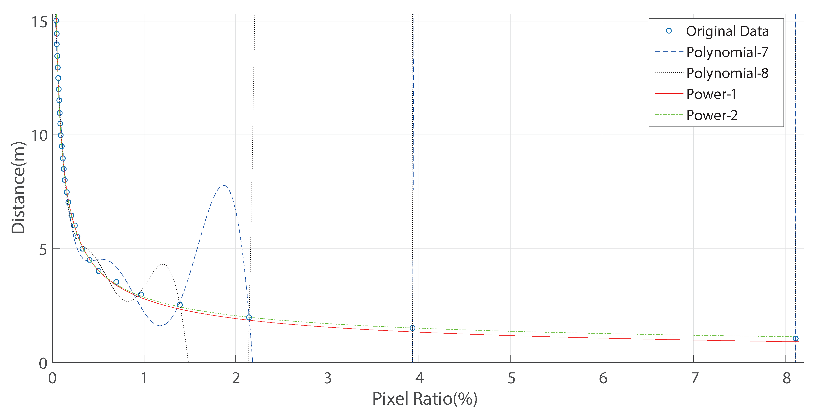
| Fitting Function | RMSE | SSE | R-Square | Adj R-sq |
|---|---|---|---|---|
| Polynomial-7 | 0.092 | 0.152 | 0.999 | 0.999 |
| Polynomial-8 | 0.067 | 0.076 | 0.999 | 0.999 |
| Power-1 | 0.117 | 0.326 | 0.999 | 0.999 |
| Power-2 | 0.100 | 0.230 | 0.999 | 0.999 |
| No. | 1 | 2 | 3 | 4 | 5 | 6 | 7 | 8 | 9 | 10 |
|---|---|---|---|---|---|---|---|---|---|---|
| SURF | 84 | 123 | 149 | 160 | 184 | 238 | 264 | 288 | 324 | 665 |
| SURF with LPSC | 35 | 26 | 35 | 54 | 60 | 69 | 106 | 105 | 106 | 249 |
| No. | 1 | 2 | 3 | 4 | 5 | 6 | 7 | 8 | 9 | 10 | |
|---|---|---|---|---|---|---|---|---|---|---|---|
| License plate | SURF | 84 | 123 | 149 | 160 | 184 | 238 | 264 | 288 | 324 | 665 |
| SURF with LNCC | 18 | 14 | 33 | 160 | 38 | 53 | 98 | 67 | 58 | 237 | |
| Logo | SURF | 36 | 40 | 46 | 65 | 84 | 95 | 104 | 114 | 137 | 169 |
| SURF with LNCC | 26 | 29 | 30 | 38 | 47 | 55 | 74 | 60 | 79 | 103 | |
| Light | SURF | 73 | 96 | 119 | 146 | 193 | 283 | 355 | 459 | 294 | 694 |
| SURF with LNCC | 33 | 77 | 88 | 113 | 141 | 197 | 234 | 312 | 195 | 403 | |
| Mirror | SURF | 26 | 27 | 29 | 29 | 36 | 48 | 48 | 50 | 79 | 99 |
| SURF with LNCC | 18 | 20 | 23 | 25 | 28 | 29 | 39 | 31 | 51 | 65 | |
| Constraint | IE (Bit/Pixel) | NMI | ||
|---|---|---|---|---|
| Left-View | Right-View | |||
| License plate | SURF | 3.5609 | 3.5549 | 0.7570 |
| SURF with LPSC | 3.1498 | 3.3349 | 0.8959 | |
| SURF with LPSC and LNCC | 3.1680 | 3.3779 | 0.8959 | |
| SURF with LPSC, LNCC and STIF | 2.7170 | 2.8372 | 0.9082 | |
| Logo | SURF | 5.0988 | 4.7373 | 0.7966 |
| SURF with LNCC | 4.7376 | 4.6422 | 0.8725 | |
| SURF with LNCC and STIF | 3.1219 | 3.1219 | 0.9359 | |
| Light | SURF | 5.8604 | 5.6467 | 0.8080 |
| SURF with LNCC | 5.6615 | 5.3441 | 0.8430 | |
| SURF with LNCC and STIF | 5.1881 | 5.0897 | 0.8991 | |
| Mirror | SURF | 3.2924 | 2.9693 | 0.9085 |
| SURF with LNCC | 2.4619 | 2.4619 | 1.0000 | |
| SURF with LNCC and STIF | 1.9219 | 1.9219 | 1.0000 | |
| No. | Satellite (km/h) | LNCC | LNCC+STIF | ||||
|---|---|---|---|---|---|---|---|
| Speed (km/h) | Error (km/h) | Speed (km/h) | Error (km/h) | Speed (km/h) | Error (km/h) | ||
| 1 | 32.40 | 32.10 | −0.30 | 32.82 | 0.42 | 33.29 | 0.89 |
| 2 | 32.40 | 32.07 | −0.33 | 31.74 | −0.66 | 31.71 | −0.69 |
| 3 | 32.44 | 33.91 | 1.47 | 31.26 | −1.18 | 31.76 | −0.68 |
| 4 | 32.47 | 32.98 | 0.51 | 32.95 | 0.48 | 32.95 | 0.48 |
| 5 | 32.44 | 33.72 | 1.28 | 33.19 | 0.75 | 32.85 | 0.41 |
| 6 | 32.40 | 33.24 | 0.84 | 32.59 | 0.19 | 33.16 | 0.76 |
| 7 | 32.31 | 31.05 | −1.26 | 33.01 | 0.70 | 32.62 | 0.31 |
| 8 | 32.31 | 32.36 | 0.05 | 33.39 | 1.08 | 33.14 | 0.83 |
| 9 | 32.34 | 32.27 | −0.07 | 32.89 | 0.55 | 32.86 | 0.52 |
| 10 | 32.31 | 31.27 | −1.04 | 32.70 | 0.39 | 32.44 | 0.13 |
| RMSE | 0.87 | 0.70 | 0.62 | ||||
| MAE | 1.47 | 1.18 | 0.89 | ||||
| MAER | 4.53% | 3.63% | 2.75% | ||||
| No. | 36 km/h | 38 km/h | 43 km/h | 45 km/h | 46 km/h | ||||||||||
|---|---|---|---|---|---|---|---|---|---|---|---|---|---|---|---|
(km/h) | LNCC (km/h) | LNCC+STIF (km/h) | (km/h) | LNCC (km/h) | LNCC+STIF (km/h) | (km/h) | LNCC (km/h) | LNCC+STIF (km/h) | (km/h) | LNCC (km/h) | LNCC+STIF (km/h) | (km/h) | LNCC (km/h) | LNCC+STIF (km/h) | |
| 1 | −0.09 | 0.10 | −1.02 | 1.79 | −0.67 | −0.95 | 0.15 | −1.62 | 0.39 | −1.89 | 1.40 | −0.94 | −1.14 | 1.03 | −1.08 |
| 2 | 1.39 | 0.79 | 0.68 | −0.16 | 0.26 | −0.91 | 1.97 | 1.01 | 1.16 | −1.09 | −0.63 | −1.31 | −0.34 | −1.04 | −1.04 |
| 3 | 0.29 | −0.71 | −0.99 | 1.31 | 0.59 | 0.53 | −0.98 | −1.36 | 0.80 | 1.87 | 1.41 | 0.93 | 0.70 | −0.69 | −1.25 |
| 4 | −0.74 | −1.14 | 0.78 | 0.35 | −1.04 | −0.56 | 1.10 | 1.35 | −0.57 | −1.07 | −0.24 | −0.84 | 0.47 | −1.12 | 0.91 |
| 5 | −0.75 | 1.00 | 0.17 | 1.63 | 1.32 | 0.77 | −0.46 | −0.75 | 1.10 | −0.08 | −0.85 | −1.24 | 0.70 | 0.32 | −1.23 |
| 6 | 1.01 | 0.38 | 0.74 | −0.13 | 1.02 | −0.68 | −0.48 | −0.44 | 0.51 | 1.07 | 1.40 | 1.09 | 0.66 | −1.19 | −0.70 |
| 7 | 1.21 | −0.91 | 0.56 | 2.23 | −0.33 | 1.08 | 1.56 | −0.93 | 0.55 | 1.26 | −1.33 | 0.76 | 0.23 | −1.28 | 0.58 |
| 8 | −0.80 | 0.95 | 0.74 | 0.17 | 0.75 | −0.54 | 0.99 | −0.55 | −0.93 | −1.89 | 0.91 | 0.72 | −1.59 | 0.71 | −0.51 |
| 9 | −0.70 | 0.77 | 0.65 | 1.44 | 1.24 | 0.63 | 0.18 | −1.04 | 0.60 | −1.63 | −1.39 | 0.46 | −1.64 | 0.62 | −1.00 |
| 10 | 1.37 | 0.76 | 0.44 | 0.37 | 0.89 | 0.87 | −1.08 | −0.39 | 0.44 | 0.77 | 1.18 | 0.25 | −1.56 | 0.80 | −0.08 |
| RMSE | 0.93 | 0.81 | 0.72 | 1.22 | 0.88 | 0.77 | 1.06 | 1.02 | 0.75 | 1.38 | 1.14 | 0.91 | 1.04 | 0.93 | 0.91 |
| MAE | 1.39 | 1.14 | 1.02 | 2.23 | 1.32 | 1.08 | 1.97 | 1.62 | 1.16 | 1.89 | 1.41 | 1.31 | 1.64 | 1.28 | 1.25 |
| MAER | 3.85% | 3.14% | 2.82% | 5.85% | 3.49% | 2.84% | 4.54% | 3.76% | 2.67% | 4.26% | 3.16% | 2.93% | 3.49% | 2.74% | 2.70% |
| No. | Logo | Light | Mirror | ||||||
|---|---|---|---|---|---|---|---|---|---|
(km/h) | LNCC (km/h) | LNCC+STIF (km/h) | (km/h) | LNCC (km/h) | LNCC+STIF (km/h) | (km/h) | LNCC (km/h) | LNCC+STIF (km/h) | |
| 1 | −0.30 | −0.98 | −0.98 | 0.59 | −1.08 | −0.76 | 19.07 | −1.85 | −1.85 |
| 2 | 0.64 | −0.70 | −0.34 | 1.48 | 1.46 | 0.79 | −2.22 | 0.63 | 0.63 |
| 3 | 1.63 | 1.18 | −0.51 | −0.40 | 0.23 | −0.73 | −11.25 | 1.01 | −0.44 |
| 4 | 0.10 | 0.63 | 0.86 | 0.24 | 0.51 | −0.22 | 6.53 | 0.65 | −0.29 |
| 5 | 0.81 | 1.12 | 0.64 | 1.43 | 0.84 | 0.86 | −5.42 | −1.39 | −0.87 |
| 6 | 0.61 | 0.33 | 0.96 | 0.68 | −1.24 | −0.80 | 0.05 | −1.92 | 1.24 |
| 7 | −0.89 | −0.94 | 0.83 | −0.01 | 0.73 | −0.84 | 3.21 | −0.79 | 1.29 |
| 8 | 1.52 | −0.56 | 0.42 | −1.25 | 0.49 | −0.93 | 9.25 | 1.39 | 0.15 |
| 9 | −0.06 | 0.47 | −0.42 | 1.34 | 1.20 | 0.54 | −8.93 | −0.65 | −0.73 |
| 10 | −0.59 | −0.46 | −0.31 | 1.40 | 0.70 | 0.08 | 1.37 | −1.87 | −0.90 |
| RMSE | 0.87 | 0.79 | 0.67 | 1.03 | 0.92 | 0.71 | 8.63 | 1.32 | 0.97 |
| MAE | 1.63 | 1.18 | 0.98 | 1.48 | 1.46 | 0.93 | 19.07 | 1.92 | 1.85 |
| MAER | 5.03% | 3.62% | 3.01% | 4.57% | 4.49% | 2.89% | 58.86% | 5.93% | 5.70% |
| Speed | Parameter | Logo | Light | Mirror | ||||||
|---|---|---|---|---|---|---|---|---|---|---|
(km/h) | LNCC (km/h) | LNCC+STIF (km/h) | (km/h) | LNCC (km/h) | LNCC+STIF (km/h) | (km/h) | LNCC (km/h) | LNCC+STIF (km/h) | ||
| 36 km/h | RMSE | 0.85 | 0.81 | 0.75 | 1.13 | 0.89 | 0.79 | 4.89 | 1.43 | 1.04 |
| MAE | 1.29 | 1.18 | 1.06 | 1.92 | 1.33 | 1.07 | 11.18 | 2.19 | 1.68 | |
| MAER | 3.57% | 3.26% | 2.91% | 5.30% | 3.66% | 2.96% | 30.96% | 5.99% | 4.65% | |
| 38 km/h | RMSE | 1.01 | 0.91 | 0.87 | 1.15 | 1.06 | 0.81 | 13.48 | 1.48 | 1.06 |
| MAE | 1.49 | 1.31 | 1.10 | 1.82 | 1.70 | 1.11 | 19.79 | 2.30 | 1.74 | |
| MAER | 3.97% | 3.44% | 2.87% | 4.86% | 4.45% | 2.92% | 52.71% | 6.20% | 4.54% | |
| 43 km/h | RMSE | 1.05 | 0.95 | 0.90 | 1.39 | 1.12 | 0.79 | 40.57 | 1.39 | 1.23 |
| MAE | 1.62 | 1.58 | 1.14 | 2.45 | 1.76 | 1.12 | 88.03 | 2.35 | 2.35 | |
| MAER | 3.71% | 3.64% | 2.63% | 5.66% | 4.06% | 2.57% | 201.53% | 5.41% | 5.41% | |
| 45 km/h | RMSE | 1.04 | 1.26 | 0.91 | 1.30 | 1.15 | 0.98 | 10.10 | 1.72 | 1.50 |
| MAE | 1.97 | 1.88 | 1.24 | 2.17 | 1.80 | 1.30 | 21.76 | 2.60 | 2.55 | |
| MAER | 4.38% | 4.17% | 2.75% | 4.84% | 4.02% | 2.88% | 48.25% | 5.80% | 5.66% | |
| 46 km/h | RMSE | 1.35 | 1.23 | 0.86 | 1.39 | 1.01 | 0.89 | 27.25 | 2.05 | 1.54 |
| MAE | 2.33 | 1.69 | 1.39 | 2.79 | 1.58 | 1.31 | 60.93 | 3.24 | 2.72 | |
| MAER | 5.01% | 3.62% | 2.96% | 5.97% | 3.39% | 2.80% | 130.88% | 6.94% | 5.92% | |
| No. | Satellite (km/h) | Plate | Logo | Light | Mirror | Average | |||||
|---|---|---|---|---|---|---|---|---|---|---|---|
| Speed (km/h) | Error (km/h) | Speed (km/h) | Error (km/h) | Speed (km/h) | Error (km/h) | Speed (km/h) | Error (km/h) | Speed (km/h) | Error (km/h) | ||
| 1 | 32.40 | 33.29 | 0.89 | 31.42 | −0.98 | 31.64 | −0.76 | 30.55 | −1.85 | 31.73 | −0.67 |
| 2 | 32.40 | 31.71 | −0.69 | 32.06 | −0.34 | 33.19 | 0.79 | 33.03 | 0.63 | 32.50 | 0.10 |
| 3 | 32.44 | 31.76 | −0.68 | 31.93 | −0.51 | 31.71 | −0.73 | 32.00 | −0.44 | 31.85 | −0.59 |
| 4 | 32.47 | 32.95 | 0.48 | 33.33 | 0.86 | 32.25 | −0.22 | 32.18 | −0.29 | 32.68 | 0.21 |
| 5 | 32.44 | 32.85 | 0.41 | 33.08 | 0.64 | 33.30 | 0.86 | 31.57 | −0.87 | 32.70 | 0.26 |
| 6 | 32.40 | 33.16 | 0.76 | 33.36 | 0.96 | 31.60 | −0.80 | 33.64 | 1.24 | 32.94 | 0.54 |
| 7 | 32.31 | 32.62 | 0.31 | 33.14 | 0.83 | 31.47 | −0.84 | 33.60 | 1.29 | 32.71 | 0.40 |
| 8 | 32.31 | 33.14 | 0.83 | 32.73 | 0.42 | 31.38 | −0.93 | 32.46 | 0.15 | 32.43 | 0.12 |
| 9 | 32.34 | 32.86 | 0.52 | 31.92 | −0.42 | 32.88 | 0.54 | 31.61 | −0.73 | 32.32 | −0.02 |
| 10 | 32.31 | 32.44 | 0.13 | 32.00 | −0.31 | 32.39 | 0.08 | 31.41 | −0.90 | 32.06 | −0.25 |
| RMSE | 0.62 | 0.67 | 0.71 | 0.97 | 0.38 | ||||||
| MAE | 0.89 | 0.98 | 0.93 | 1.85 | 0.67 | ||||||
| MAER | 2.75% | 3.01% | 2.89% | 5.70% | 2.08% | ||||||
| Speed | Parameter | Plate (km/h) | Logo (km/h) | Light (km/h) | Mirror (km/h) | Average (km/h) |
|---|---|---|---|---|---|---|
| 36 km/h | RMSE | 0.72 | 0.75 | 0.79 | 1.04 | 0.30 |
| MAE | 1.02 | 1.06 | 1.07 | 1.68 | 0.54 | |
| MAER | 2.82% | 2.91% | 2.96% | 4.65% | 1.48% | |
| 38 km/h | RMSE | 0.77 | 0.87 | 0.81 | 1.06 | 0.54 |
| MAE | 1.08 | 1.10 | 1.11 | 1.74 | 1.06 | |
| MAER | 2.84% | 2.87% | 2.92% | 4.54% | 2.79% | |
| 43 km/h | RMSE | 0.75 | 0.90 | 0.79 | 1.23 | 0.37 |
| MAE | 1.16 | 1.14 | 1.12 | 2.35 | 0.77 | |
| MAER | 2.67% | 2.63% | 2.57% | 5.41% | 1.77% | |
| 45 km/h | RMSE | 0.91 | 0.91 | 0.98 | 1.50 | 0.40 |
| MAE | 1.31 | 1.24 | 1.30 | 2.55 | 0.90 | |
| MAER | 2.93% | 2.75% | 2.88% | 5.66% | 1.99% | |
| 46 km/h | RMSE | 0.91 | 0.86 | 0.89 | 1.54 | 0.43 |
| MAE | 1.25 | 1.39 | 1.31 | 2.72 | 0.84 | |
| MAER | 2.70% | 2.96% | 2.80% | 5.92% | 1.79% |
Publisher’s Note: MDPI stays neutral with regard to jurisdictional claims in published maps and institutional affiliations. |
© 2021 by the authors. Licensee MDPI, Basel, Switzerland. This article is an open access article distributed under the terms and conditions of the Creative Commons Attribution (CC BY) license (https://creativecommons.org/licenses/by/4.0/).
Share and Cite
Yang, L.; Li, Q.; Song, X.; Cai, W.; Hou, C.; Xiong, Z. An Improved Stereo Matching Algorithm for Vehicle Speed Measurement System Based on Spatial and Temporal Image Fusion. Entropy 2021, 23, 866. https://0-doi-org.brum.beds.ac.uk/10.3390/e23070866
Yang L, Li Q, Song X, Cai W, Hou C, Xiong Z. An Improved Stereo Matching Algorithm for Vehicle Speed Measurement System Based on Spatial and Temporal Image Fusion. Entropy. 2021; 23(7):866. https://0-doi-org.brum.beds.ac.uk/10.3390/e23070866
Chicago/Turabian StyleYang, Lei, Qingyuan Li, Xiaowei Song, Wenjing Cai, Chunping Hou, and Zixiang Xiong. 2021. "An Improved Stereo Matching Algorithm for Vehicle Speed Measurement System Based on Spatial and Temporal Image Fusion" Entropy 23, no. 7: 866. https://0-doi-org.brum.beds.ac.uk/10.3390/e23070866