
Modelling of the Electrical Membrane Potential for Concentration Polarization Conditions
by
 , ,
, ,
Kornelia M. Batko
1,* ,
,
Izabella Ślęzak-Prochazka
2 ,
,
Andrzej Ślęzak
3, 
Wioletta M. Bajdur
4,* and
Radomir Ščurek
5
1
Department of Business Informatics, University of Economics in Katowice, 2B Bogucicka, 40287 Katowice, Poland
2
Biotechnology Centre, Silesian University of Technology, Akademicka 2A, 44100 Gliwice, Poland
3
Department of Health Science, Jan Dlugosz University, 13/15 Armia Krajowa Al., 42200 Częstochowa, Poland
4
Faculty of Management, Częstochowa University of Technology, 35b Armia Krajowa Al., 42200 Częstochowa, Poland
5
Department of Security Services, Faculty of Safety Engineering, VŠB-Technical University of Ostrava, ul. Lumirova 3, 70030 Ostrava, Czech Republic
*
Authors to whom correspondence should be addressed.
Entropy 2022, 24(1), 138; https://0-doi-org.brum.beds.ac.uk/10.3390/e24010138
Submission received: 10 December 2021
/
Revised: 29 December 2021
/
Accepted: 7 January 2022
/
Published: 17 January 2022
(This article belongs to the Section Thermodynamics)
Abstract
:Based on Kedem–Katchalsky formalism, the model equation of the membrane potential () generated in a membrane system was derived for the conditions of concentration polarization. In this system, a horizontally oriented electro-neutral biomembrane separates solutions of the same electrolytes at different concentrations. The consequence of concentration polarization is the creation, on both sides of the membrane, of concentration boundary layers. The basic equation of this model includes the unknown ratio of solution concentrations ( at the membrane/concentration boundary layers. We present the calculation procedure ( based on novel equations derived in the paper containing the transport parameters of the membrane (, , and ), solutions (, ), concentration boundary layer thicknesses (, ), concentration Raileigh number (), concentration polarization factor (), volume flux (), mechanical pressure difference (), and ratio of known solution concentrations (). From the resulting equation, was calculated for various combinations of the solution concentration ratio (), the Rayleigh concentration number (), the concentration polarization coefficient (), and the hydrostatic pressure difference ). Calculations were performed for a case where an aqueous NaCl solution with a fixed concentration of 1 mol m−3 () was on one side of the membrane and on the other side an aqueous NaCl solution with a concentration between 1 and 15 mol m−3 (). It is shown that () depends on the value of one of the factors (i.e., , , and ) at a fixed value of the other three.
1. Introduction
Both biological and synthetic membranes are sensitive to changes in the physicochemical properties of the environment [1,2,3,4]. Therefore, membrane transport of its solution components can be governed by local fields (such as concentration, temperature, electric potential, or pressure fields) and global fields (such as gravitational or electromagnetic fields) [1,5]. Under real-world conditions (no external mixing of membrane-separated solutions), concentration polarization plays an important role, involving the formation of concentration boundary layers in solution regions immediately adjacent to the membrane [6,7,8,9]. In electrochemistry, the term concentration polarization is used to describe a set of phenomena accompanying the formation of concentration gradients in electrolyte solutions adjacent to a semipermeable solid/liquid interfacial surface during the flow of an electric current and the appearance of a boundary current [10,11,12,13,14].
The term concentration polarization is also used to describe the phenomena accompanying the formation of concentration boundary layers (CBLs) in both electrolyte and non-electrolyte solutions [3,4,7,8,9,15,16,17]. The effect of concentration polarization is to reduce membrane transport [7,8,9,16,17]. These layers are formed on both sides of electrically neutral selective membranes oriented horizontally, and the concentration (density) gradients in them are sensitive to the gravitational field [1,7,15,16,17]. The effect of this field is natural convection, which modifies the concentration fields in the membrane regions [7,15]. Its consequence is a partial restoration of concentration gradients across the membrane and increased membrane transport [3,16,17]. One of the effects of changing the concentration field are gravitational effects in passive osmotic and diffusive transport [1,18,19] and the gravielectric effect [16]. Theoretical modeling of the concentration polarization phenomenon is usually based on the Kedem–Katchalsky and Nernst-Planck equations [14,20,21,22,23].
The gravielectric effect in an electrochemical cell is a consequence of diffusion, concentration polarization, and the action of gravity [16]. In this study, we used a system in which two solutions with different NaCl or KCl solutions were separated by a synthetic membrane. The solutions were connected to Ag/AgCl electrodes using original bridges [16] or immersed directly into the solutions [24,25,26]. Furthermore, mathematical models of this effect were developed using the Kedem–Katchalsky equations [24,25,26]. In the first case, the dependence of the measured difference of electric potentials on the distance of electrodes from the membrane was eliminated. In the second case, the dependence was obvious. These studies showed, among other things, that the reversal of the mechanical pressure gradient with respect to the concentration (density) gradient has a significant effect on the value of the membrane potential difference [26].
The decrease in fluxes and thermodynamic forces due to the concentration polarization commonly found in nature, contributes to slowing down the source of entropy. This is an anti-entropic process.
The aim of this paper was to develop model equations of the membrane potential difference () for concentration polarization conditions based on Kedem–Katchalsky formalism. The basic equation of this model includes the unknown ratio of solution concentrations ( at the membrane/concentration boundary layers. We present the calculation procedure ( based on the novel equations derived in the paper containing the transport parameters of the membrane (, , and ), solutions (, ), concentration boundary layer thicknesses (, ), concentration Raileigh number (), concentration polarization factor (), volume flux (), mechanical pressure difference (), and ratio of known solution concentrations (. We used the obtained equation to calculate the characteristics and . The characteristics were calculated for different fixed values of , , and . In contrast, the characteristics were calculated for different fixed values of ,, and , while the characteristics were calculated for different fixed values of , and .
2. Materials and Mathematical Modeling
2.1. Membrane System
In this paper, the considerations were based on the membrane system schematically shown in Figure 1. In this system, two mechanically unstirred solutions of the same electrolyte were separated by a hemodialyzer biomembrane (i.e., Nephrophan) made of regenerated cellulose (M), oriented in the horizontal plane. Nephrophan (Orwo VEB Filmfabrik, Wolfen, Germany) is a microporous, highly hydrophilic, isotropic, homogeneous, symmetric, and electro-neutral membrane [27]. The transport properties of a thick membrane are determined by the following coefficients: hydraulic conductivity (), reflection (), solute permeability (), electrical conductivity (), and transfer number (). At the initial time (), the concentrations of these solutions were and ( > ). For , water and solute diffusing through the membrane form on both sides of the membrane concentration boundary layers and with thicknesses of and , respectively. These layers can be perceived as membranes with diffusion coefficients and , reflection coefficients = = 0, transfer numbers and , and electrical conductivity coefficients and . The membrane together with the concentration boundary layers form the /M/ complex. The transport properties of this complex are determined by the following coefficients: reflection (), solute permeability (), electrical conductivity (), and the transfer number (). The process of creating concentration boundary layers causes the concentration of the solution on the M/ border to increase from to ( > ) and on the /M border to decrease from to ( > ).
The solute flux and ionic current through the layer are denoted by and , respectively, through the M membrane by and and through the layer by and . The volume, solute, and ion current fluxes through the /M/ complex are denoted by , , and , respectively. It is worth noting that it is possible to select the concentrations of the solutions in such a way that the concentration gradient and the density gradient are parallel or antiparallel to the gravity vector. Interferometric studies have shown that the formation of the layers and ends when natural convection occurs, and the membrane system reaches a steady state.
2.2. Equations for Fluxes and Concentration Polarization Conditions
For electrically neutral membranes, the results of membrane transport studies of electrolyte solutions can be interpreted based on Kedem–Katchalsky formalism [22,23,27]. In this formalism, the membrane is treated as a “black box”, and its properties are described by the relationship between the thermodynamic forces (which cause the permeation of solution components through the membrane) and the thermodynamic fluxes that result from these forces. For binary electrolyte solutions, the Kedem–Katchalsky equations are of the form [23,24]:
where —volume flux; —solute flux; —ion current; , , and and —coefficients of hydraulic conductivity, reflection, electroosmotic permeability, and solute permeability, respectively; γ—van’t Hoff coefficient; RT—the product of the gas constant and the absolute temperature; and —solution concentrations ( > ); —electrical conductivity; , , and —transfer number, valence, and ion number, respectively; —average concentration of the solution ( is only valid when the and values are not very different); —potential difference measured with two reversible electrodes; , , and —transfer numbers of anions (a) and cations (c) in the membrane, respectively; .
Equations (1)–(4) are correct for sufficiently dilute and homogeneous solutions [23,24]. As already mentioned, when the solutions are not mechanically mixed, CBLs form on both sides of the membrane [4,6,15,16,17,18]. These layers can be thought of as pseudomembranes connected in series with the material membrane. The consequence of the formation of these layers is a decrease in membrane transport, which is manifested by a decrease in volume flux, solute flux, membrane potential, and ionic current [1,4,6,15,16,17].
Based on the classical [22,23] and modified [28,29] form of Equation (2) and the amperostatic condition , we can write:
where —the concentration polarization coefficient, —the hydraulic volume flux, and —osmotic volume flux.
In the steady state, the condition is fulfilled by:
Equations (5)–(7) and (9) are used to calculate the solution stabilities at the boundaries M/ () and /M (), assuming that = = 0:
For isoosmotic conditions (, = ), Equations (10) and (11) simplify to the form:
For = 0, and therefore Equations (10) and (11) will take the form
2.3. Equations for the Concentration Rayleigh Number
The process of creating concentration boundary layers is controlled by the Rayleigh concentration number () [15]. For the membrane system in question, containing concentration boundary layers and with thicknesses and , the expressions for the concentration Rayleigh numbers take the forms:
where g is acceleration due to the fact of gravity, and are the mass density of solutions ( > ), and are the kinematic viscosity of the solutions ( > ), and are the layer and thicknesses, and are the diffusion coefficients in the layers and , and are the kinematic viscosity coefficients ( > ), and represent the change in density of a solution due to the change in the solution concentration, and and represent the density gradient along the vertical axis. When the density of the solution above the membrane is greater than the density of the solution below the membrane, convective instabilities appear in the membrane regions when the values of and exceed their critical values. For membrane transport processes, the critical value of the = 1100.6 [30]. In the linear case, that is, when = and = , Equations (16) and (17) can be written in the form [31]:
where and are the solution densities at the boundaries of M/ and M/ ( > ), and and are the solution densities beyond and ( > ).
In order to estimate and at steady state, we carried out the following considerations. Assuming that for small concentrations of solutions the density–concentration dependence is linear, we can write:
where and are the densities of the solution and solvent, respectively, and ) = const. For binary solutions, the above equation takes the form:
Considering Equations (10) and (11) in Equations (21) and (22) and then in Equations (18) and (19), we obtain concentration Rayleigh numbers (, ) for isothermal processes of passive membrane transport
For = 0 and ; therefore, Equations (23) and (24) take the form:
2.4. Membrane Potential Equations for Concentration Polarization Conditions
Using the procedure presented in the previous paper [4], for the situation presented in Figure 1, Equation (4) can be written in the following forms:
In the steady state, the following conditions are fulfilled:
Based on Equations (29) and (30) and the condition = = , we obtain:
where , , and .
In order to represent the ratio in a form suitable for calculation, we form the quotient of the left and right sides of Equations (10) and (11). After performing the appropriate algebraic transformations, we obtain:
where
For the denominator of this equation to be greater than zero, the following condition must be fulfilled: > 0. For = 0, Equation (35) takes the form:
For the denominator of this equation to be greater than zero, the following condition must be fulfilled:
If we neglect the osmotic effects ( << , we obtain from Equation (35):
2.5. Equations for the Thickness of the Concentration Boundary Layers
The equations for and can be obtained by transforming Equations (27) and (28) into the forms:
where , , , , , and . If we neglect the osmotic effects ( << , << ), considering the equation = in Equations (38) and (39) we obtain:
where , , , , , and . To obtain the equations describing and for isoosmotic conditions (, = ), it is sufficient to transform Equations (25) and (26) into the forms:
Expressions (35), (36) and (38)–(41) constitute the equations describing the membrane potential generated in a membrane system containing an isotropic, symmetric, and electron neutral polymer membrane for the conditions of concentration polarization.
3. Results of Calculations and Discussion
Calculations of the membrane potential () were made based on Equations (34), (35), (40) and (41) for a membrane system characterized as follows. The membrane was positioned on a horizontal plane and separated by two aqueous NaCl solutions with concentrations of = 1 mol m−3 and = , where = 1.25 mol m−3 and = 1, 2, …, 8. For the density () and kinematic viscosity () the following relationships were satisfied: = + and = + , where = 997.4 kg m−3, = 0.03.4 kg m−3, = 997.7 × 10⁻⁹ m2s−1, = −0.03 × 10⁻⁹ m2s−1, and = 1, 2, …, 8. The concentration gradient density calculated on the basis of the above data was () = 0.026 kg mol−1. It was assumed that the diffusion coefficient of NaCl in the range of tested solution concentrations was constant ( = ) and, therefore, the table value = 1.57 × 10⁻⁹ m2s−1 was used for the calculations. For the calculations, the transport parameters of the Nephrophan membranes used as an element of the hemodialyzer were used [32] for NaCl with the following values: = 5 × 10⁻¹² m3N−1s−1, = 0.06, = 1.43 × 10⁻⁹ mol N−1s−1, = 0.39, and = 0.216 [16]. The values of the coefficient assume values in the range . Moreover, the constants = 8.31 J mol−1K−1, = 9.81 m s−1, and = 9.65 × 10⁵ C mol−1 were used for the calculations. The calculations were made using the MATLAB software package. All calculations were made for isothermal conditions ( = 295 K). The characteristics for different set values of ,, and are shown in Figure 2. The characteristics for different set values of ,, and are shown in Figure 3. Figure 4 shows the characteristics of for different fixed values of ,, and .
3.1. Concentration Dependence of Membrane Potential
Figure 2a shows the characteristics of for the same value and of different set values of . This figure shows that the curves (1)–(5) start from a point with the coordinates = 1 and = 0. Curve (1) shows that is positive over the entire range of the values. Curve (2) shows that fulfilled the following conditions: = 3.85, = 0; < 3.85, < 0. For curves (3)–(5), < 0.
Figure 2b shows that the change of the sign of and the value of and the change of the set values of caused a change in the nature of the curves, illustrating the dependence . This figure shows that the curves (1)–(5) started from different positive values of . The curves (1)–(3) show that was positive for the entire range of values. The course of the curves (4) and (5) shows that fulfilled the following conditions: ≈ 2.65, = 0; < 2.65, < 0; > 2.65, > 0. For curves (3)–(5), < 0.
Figure 2c shows two families of the characteristics . The first is illustrated by the curves (1)–(3), the second by the curves (4)–(6). The course of the curves (1)–(3) shows that with the increase in the value of , the value of increased nonlinearly. The shape of the curves for the same values depended on the value. Curve (1), in the tested interval , was a characteristic of the saturation type. The change in the type of the mentioned characteristic from (1) to (2) and (3), controlled by the value, occurred for ≥ 18.
The average slope of the characteristics can be calculated from the expression . For 1 ≤ < 18, the value of was constant and approximately = 1.65 mV (for curve (1)), = 3.5 mV (for curve (4)), and = 4 mV (for curve (3)). For ≥ 18, the value of was constant and amounted to approximately = 2 mV (for curve 1), = 20 mV (for curve (2)), and = 85 mV (for curve (3)). This means that for > 200, there was an almost abrupt increase in the value of . The comparison of curves (1) and 3 for > 18 shows that the value of the coefficient for curve (3) was 42.5 times greater than the value of the coefficient for curve (1). In turn, curves (4)–(6) show that that with the increase in the value of , decreased nonlinearly, and for = 3.48, it reached the minimum value of = 0.225 V. For > 3.48, increased. Similarly, as in the previous case, it was possible to calculate the average slope of the characteristics . For 1 ≤ > 3.48, the value of for curves (4)–(6) was constant and amounted to approximately = 1.11 mV. For < 3.48, the value of was constant and approximately = −167 mV (for curve (3)), = −44 mV (for curve 2), and = −7.1 mV (for curve (1)). The comparison of curves (1) and (3) for < 3.48 shows that the value of the coefficient for curve (3) was 23.5 times greater than the value of the coefficient for curve (1).
Figure 2d shows two groups of characteristics for + (curves (1a)–(5a)) and – (curves (1b)–(5b)). These characteristics differed from the characteristics shown in Figure 2a–c because curves (1a),(2a), (3a), (4a), (1b), (2b), (3b) and (4b), illustrating the dependencies had minima , for which the value decreased as the value increased. The curves (5a) and (5b) did not have minima, because for = 4423.6023 (curves (5b)) and = 0.6023 (curves (5a)). This is because Equation (31) has no solutions in the set of real numbers.
3.2. Hydrostatic Pressure Dependencies of Membrane Potential
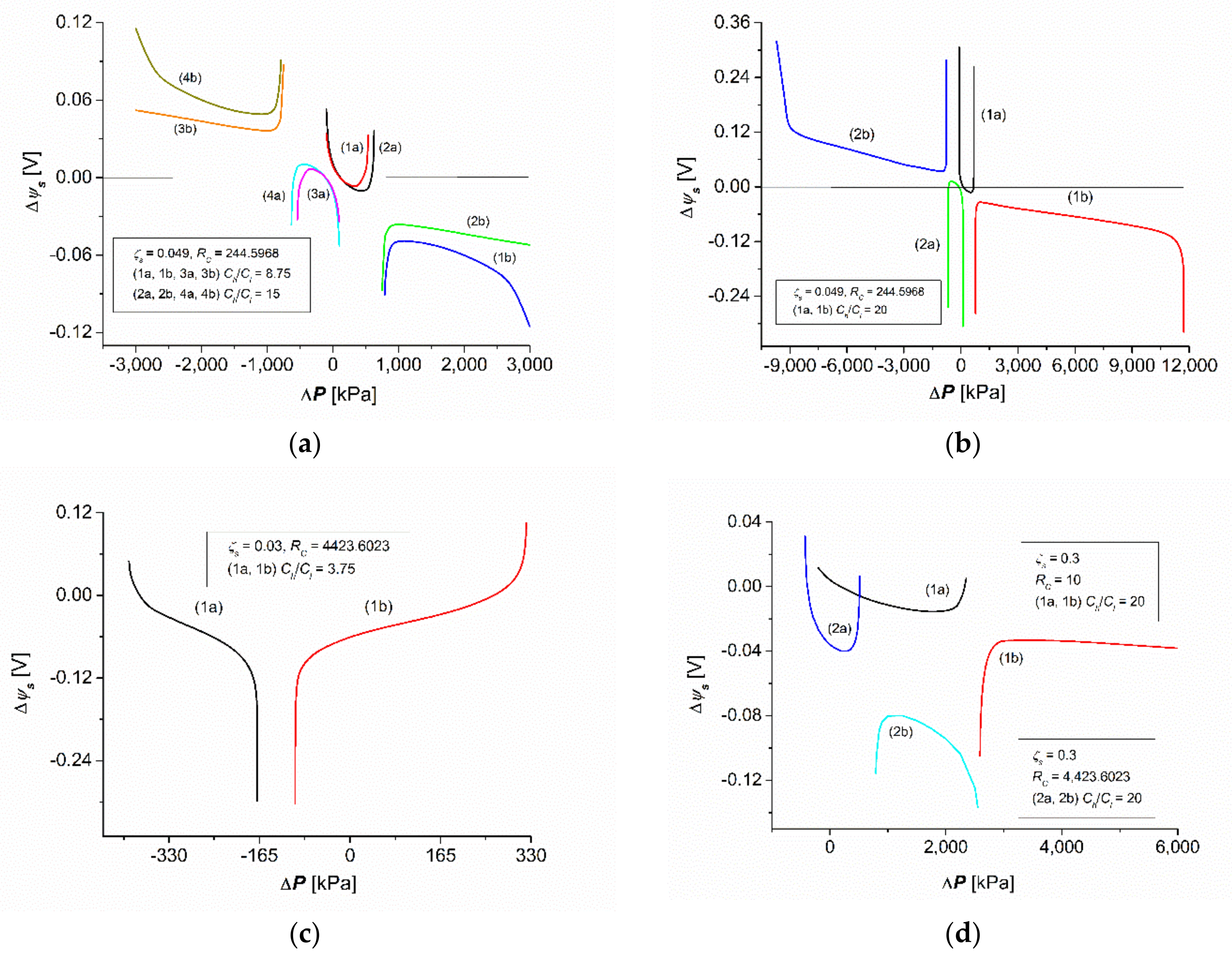
Figure 3 shows the characteristics calculated for the set values of = 0.049, = 244.5968, = 8.75 (curves (1a,b) and (3a,b) in Figure 3a), and = 15 (curves (2a,b) and 4a,b in Figure 3a)). These figures show that in the tested interval (i.e., , and , Equation (31) had two solutions. Let us consider the curves (2a,b) shown in Figure 3a, illustrating two solutions for Equation (31) in the set of real numbers. The coordinates of the point determining the minimum of curve (1a) are as follows: = 0.103 V and = 0.478 MPa. In turn, the coordinates of the point determining the maximum of curve (1b) are as follows: = −0.064 V and = 1.275 MPa. The coordinates of the point determining the minimum of the curve (2a) are = 0.1 V and = 0.5 MPa. In turn, the coordinates of the point determining the maximum of curve 2b are as follows: = −0.086 V and = 1.55 MPa. This means that the change from = 8.75 to = 15 shifts curve (2a) in relation to curve (1a) towards higher values of ΔP and lower values of . In turn, the change from = 8.75 to = 15 shifts curve (2b) in relation to curve (1b) towards lower values of and higher values of . Moreover, curves (1a) and (2a) are symmetrical to curves (3a) and (4a) as are curves (1b) and (2b) to curves (3b) and (4b).
Curve (1a), as depicted in Figure 3b, shows that the range of changes falls on a relatively narrow range that meets the condition −78 ≤ ≤ 700 kPa. In the case of the curve (1b) presented in this figure, it follows that the range of changes is within the wide range , which satisfies the condition −780 kPa ≤ ≤ 11.7 MPa. Curve (1a) had had a minimum at the coordinate = −0.012 V and = 0.545 MPa. In turn, curve (1b) had a maximum at the coordinates = −0.034 V and = 1.052 MPa.
Figure 3c shows the characteristics calculated for the set values = 0.3, = 4423.6023, and = 3.75 (curves (1a,b) in Figure 3c). This figure shows that in the tested interval (i.e., , and ), Equation (31) had two solutions. The first is illustrated by curve (1a), and the second is shown by curve (1b). The curves presented in Figure 3c show that the curve (1a) was asymmetric in relation to curve (1b). Curve (1a) presented in Figure 3c shows that the range of changes was within the ΔP interval, which satisfies the condition −300 ≤ ≤ −170 kPa. In this range , the value of decreased nonlinearly from = 0.05 V to = −0.3 V. In turn, in the case of curve (1b), the range of changes was within the range , satisfying the condition −100 ≤ ≤ +300 kPa. In this case, the value of decreases nonlinearly from = −0.3 to = +0.107 V.
Curve 1a, as depicted in Figure 3d, shows that the range of changes was in the interval, which satisfies the condition −0.45 ≤ ≤ +0.514 MPa. This curve had a minimum at the point with the coordinates = −0.04 V and = 0.3 MPa. Moreover, this curve shows that with the increase in , the value of decreased nonlinearly until reaching the minimum value and then increased nonlinearly. On the other hand, in the case of curve (1b), the range of changes of was within the range, which satisfies the condition of 0.78 ≤ ≤ +2.54 MPa. This curve had a maximum at the coordinates = −0.08 V and = 1.12 MPa. Moreover, this curve shows that with the increase in , the value of increased nonlinearly until reaching the maximum value and then decreased nonlinearly.
The curves 2a,b shown in Figure 3d illustrate the dependence , calculated based on Equation (31) for the determined values = 0.3, = 10, and = 20. This figure shows that in the examined interval , and ), Equation (31) had two solutions, which are graphically illustrated by the curves (2a,b). Curve (2a) shows that the range of changes was in the ΔP range, which satisfies the condition of −280 kPa ≤ ≤ +2.33 MPa. This curve had a minimum at the point with coordinates = −0.015 V and ( = 1.85 MPa). Moreover, this curve shows that with the increase in , the value of decreased nonlinearly until reaching the minimum value and then increased nonlinearly. On the other hand, in the case of curve (1b), the range of changes of was within the range, which satisfies the condition of 2.6 ≤ ≤ 6.0 MPa. This curve had a maximum at the coordinates = −0.032 V and = 3.5 MPa. Moreover, this curve shows that with the increase in , the value of increased nonlinearly until reaching the maximum value and then decreased nonlinearly.
3.3. Rayleigh Number Dependencies of Membrane Potential
Figure 4 shows the characteristics of for various fixed values of ,, and . Figure 4a shows for the same value = +100 kPa and = 0.049 for different set values of . The calculation results illustrated by the curve presented in Figure 4a show that the value of increased nonlinearly with the increase in the value. This means that this increase was different in different ranges. For 0 < < 6333.3, the tangent of the slope of the tangent to the curve segment was approximately constant and amounted to / = 6.8 μV. In turn, for 6333.3 ≤ ≤ 6729.2, the tangent of the slope of the tangent to the curve segment was approximately constant and amounted to = 0.27 mV. Hence, it follows that the ratio of the tangent slopes of the tangents to the discussed sections of curve (1), as shown in Figure 4a, was approximately 400. This means that after crossing the point with the coordinates = 0.04 V and = 6333.3, the kinetics of membrane transport change abruptly. It should be noted that for the tested range, all values were positive.
Curves (2–4), depicted in Figure 4a, show that an increase in the value of while maintaining the values of and , changes the course of the characteristic from nonlinearly increasing (curve in Figure 3a) to nonlinearly decreasing (curves 2, 3, and 4 in Figure 4a). Moreover, for the tested range, the values were both positive and negative. It should also be noted that in the case of curve (2), in the range of small values, as the value increased, initially decreased quickly and then, after reaching the minimum value, ()min = −0.002 V for = 1800, slowly grew. Curves (3) and (4) are nonlinearly decreased, but in the case of curve (4), the decrease in the value of the potential caused by the increase in the value of was significantly faster than in the case of curve (3).
Figure 4b shows the characteristics calculated for the set values = +100 kPa, = 20, and = 0.049 (curve (1)) and = 0.049 (curve (2)). The course of these curves shows that an increase in the value causes a nonlinear decrease in the value of . Moreover, takes both positive and negative values. This decrease in value is greatest for 0 < < 265 and it decreases for higher values of . It should be noted that an increase in the value of shifts the curves towards smaller values of .
Figure 4c shows the characteristics calculated for the set values = −100 kPa, = 20, and = 0.049 (curve 1), = 0.055 (curve (2)), and = 0.058 (curve 3). The course of these curves shows that an increase in the value caused a nonlinear increase in the value of and that was positive. Moreover, it should be noted that an increase in the value of shifted the abovementioned curves towards higher values of . Within curves 1–3, three segments can be distinguished: the first—linear, the second—nonlinear, and the third—linear. The tangents to the linear segments of these curves intersected at the following coordinates: = 0.078 V and = 228.57 (curve (1)); = 0.077 V and = 779.22 (curve (2)); = 0.077 V and = 1641.56 (curve (3)). This means that after crossing this point, the kinetics of membrane transport changes abruptly. The tangents of the angles of inclination of the first linear sections of curves (1–3) were, respectively, ()/ = 0.19, 0.056, and 0.026 mV. This means that the value of this tangent decreased with the increasing value of . In turn, the tangents of the angles of inclination of the second linear sections of curves (1–3) were, respectively, ()/ = 20, 19, and 17 mV. In addition, in this case, the value of this tangent decreased with an increasing value. These data also show that the tangent ratio of the angles of inclination for the second and first sections of the curves 1–3 were 105.339 and 654, respectively. This means that the value of this ratio decreased with an increasing value of .
Figure 4d shows the characteristics , calculated for the different set values of . The curves in this figure are of a similar shape. The values of ( illustrated by curve (1) were independent of for 0 ≤ ≤ 0.05. For > 0.05, the value of ( increased until the maximum value was reached at the point with coordinates = 0.83 and = 0.122. After reaching the maximum value, the value of decreased nonlinearly until reaching = 0, for > 0.6. The values of illustrated by curve (2) increased until the maximum value was reached at the point with coordinates = 0.2 and = 0.206. After reaching the maximum value, the value of decreased nonlinearly until reaching = 0, for > 0.6.
In summary, the results of calculations based on Equations (34), (35), (40) and (41), presented in Figure 2, Figure 3 and Figure 4, show that the membrane potential for concentration polarization conditions depends on the value of one of the four factors—, (), , and —at fixed values of the other three.
3.4. Discussion
Equations (1)–(3) show that for = 0, four processes were involved in the creation of the characteristics shown in Figure 1, Figure 2, Figure 3 and Figure 4: hydraulic flow, osmosis, diffusion, and advection. In the studied range of and , the role of the osmotic agent in the creation of was negligibly small. To demonstrate this, let us consider the equation describing the osmotic flux. Considering in this equation, the data = 5 × 10⁻¹² m3N−1s−1, = 0.06, = 2.45 × 10³ J mol−1, and = 12.5 mol m−3, we obtain = 0.9 × 10⁻⁸ m s−1. For isoosmotic conditions, = . This condition corresponds to = 1.8 kPa. For >> and << . This means that the influence of osmosis on the creation of was negligibly small and the mechanical pressure was large. In order to show what the contribution of the diffusion and advection factor in the creation of , let us consider Equations (1) and (2). If we consider Equation (1) in Equation (2) we obtain:
where —diffusion flux, —advective (osmotic) flux, and —advective (hydraulic) flux.
By substituting appropriate values into Equation (44), it can be shown that >> , because = 4 × 10⁻⁵ mol m−2s−1, = 3 × 10⁻⁹ mol m−2s−1, and . This means that the effect of osmosis on diffusion and, therefore, on the creation of was negligibly small. In turn, . Given the relevant data, one can show that if = = 4 × 10⁻⁵ mol m−2s−1, then = 1.9 × 10⁶ kPa. For >> , the effect of pressure advection on diffusion and, thus, on the creation of was large. From the above discussion, it is clear that due to the organic range of () and the unlimited range of , only molecular diffusion and hydraulic advection are involved in the creation of .
4. Conclusions
This paper presented an equation describing the membrane potential generated in a membrane system (containing an isotropic, symmetric, and electronically inert polymer membrane) for concentration polarization conditions. This equation for currentless conditions ( = 0) has the form:
where
This is an equation that is the sum of two logarithmic expressions. The second component is particularly complex, because it contains components with different powers, ranging from fractional to quadratic. The above equation certainly has many different solutions, depending on the parameters regarding the transport properties of the membrane and the physicochemical and hydrodynamic properties of the solutions it separates. Figure 2, Figure 3 and Figure 4 show examples of solutions in the form of the dependence: for different fixed values of ,, and ; for different fixed values of ,, and ; for different fixed values of ,, and . Certainly, the curves presented in Figure 2, Figure 3 and Figure 4 do not exhaust all types of solutions to Equation (21).
It can be seen from the relationships in these figures that changing the values of ,, , and/or causes a change in the type of characteristic. This means that is sensitive to a factor (e.g., environmental forces), the source of which is the thermodynamic environment of the membrane. Biological membranes, which are the microscale equivalent of our skin, behave in a similar but more complex way [2]. The membrane has embedded switches that respond to physical signals from the environment, relaying information to intracellular protein pathways. Almost every environmental signal recognized by a cell has a different switch in the cell membrane. What these switches have in common is a similar design and method of operation.
Undoubtedly, synthetic membranes used as an active dressing component in the treatment of hard-to-heal wounds, such as extensive burns or venous leg ulcers, are a skin substitute [32]. In this process, the membrane serves as a barrier that creates an appropriate microenvironment between the wound and the membrane surface. The physiological environment thus created contributes to faster wound healing, which has both medical and economic dimensions.
Author Contributions
Conceptualization, K.M.B. and A.Ś.; methodology, K.M.B., A.Ś. and I.Ś.-P.; software, K.M.B.; formal analysis: K.M.B., A.Ś., I.Ś.-P. and W.M.B.; investigation, K.M.B., A.Ś. and I.Ś.-P.; resources, K.M.B., A.Ś., I.Ś.-P. and W.M.B.; data curation, K.M.B. and A.Ś.; writing—original draft preparation, K.M.B., A.Ś., I.Ś.-P., R.Ś. and W.M.B., writing—review and editing, K.M.B., A.Ś., I.Ś.-P., W.M.B. and R.Ś.; visualization, K.M.B. and A.Ś.; supervision, A.Ś.; funding acquisition, R.Ś. and W.M.B. All authors have read and agreed to the published version of the manuscript.
Funding
The scientific research was funded by the statute subvention of Czestochowa University of Technology.
Institutional Review Board Statement
Not applicable.
Informed Consent Statement
Not applicable.
Data Availability Statement
The data sets for this study are available upon request from the corresponding author.
Acknowledgments
We would like to thank those who have touched our science paths.
Conflicts of Interest
The authors declare no conflict of interest.
List of Symbols
| volume flux (m s−1) | |
| Jl, Jm, Jh | solute fluxes; (mol m−2s−1) |
| Il, Is, Im, Ih | ionic currents (A) |
| hydraulic conductivity coefficient (m−3N−1s−1) | |
| reflection coefficient | |
| electroosmotic permeability coefficient (NA−1) | |
| solute permeability coefficient (mol N−1s−1) | |
| γ | van’t Hoff coefficient |
| R | gas constant (J mol−1K−1) |
| T | absolute temperature (K) |
| electrical conductivity (Ω−1m−2) | |
| transfer number | |
| valence | |
| ion number | |
| average concentration of the solution (mol m−3) | |
| potential difference measured with two reversible electrodes (V) | |
| , | transfer number of anions (a) and cations (c) in the membrane |
| time (s) | |
| and | concentration boundary layers |
| δl, δh | thickness of the concentration boundary layers (m) |
| δm | membrane thickness (m) |
| mechanical pressure difference (Pa) | |
| CBLs | concentration boundary layers |
| g | acceleration due to the fact of gravity (m s−2) |
| , | diffusion coefficients (m2s−1) |
| , | the kinematic viscosity coefficients (m2s−1) |
| , | solution concentrations at the boundaries of M/ and M/ (mol m−3) |
| , | solution densities at the boundaries of M/ and M/ (kg m−3) |
| , | solution concentrations beyond and (mol m−3) |
| , | solution densities beyond and (kg m−3) |
References
- Batko, K.M.; Ślęzak, A.; Bajdur, W.M. The role of gravity in the evolution of the concentration field in the electrochemical membrane cell. Entropy 2020, 22, 680. [Google Scholar] [CrossRef]
- Lipton, B.H.; Bhaerman, S. Spontaneous Evolution–Our Positive Future and a Way to Get There from Here; Hay House Inc.: Carlsbad, CA, USA, 2018; ISBN 1401923127. [Google Scholar]
- Batko, K.M.; Ślęzak, A. Evaluation of the global S-entropy production in membrane transport of aqueous solutions of hydrochloric acid and ammonia. Entropy 2020, 22, 1021. [Google Scholar] [CrossRef]
- Ślęzak, A.; Ślęzak, I.H.; Ślęzak, K.M. Influence of the concentration boundary layers on membrane potential in a single-membrane system. Desalination 2005, 184, 113–123. [Google Scholar] [CrossRef]
- Bruinsma, R.; Aleksander, S. Theory of electrohydrodynamic instabilities in electrolytic cells. J. Chem. Phys. 1990, 92, 3074–3080. [Google Scholar] [CrossRef]
- Barry, P.H.; Diamond, J.M. Effects of unstirred layers on membrane phenomena. Physiol. Rev. 1984, 64, 763–872. [Google Scholar] [CrossRef]
- Dworecki, K.; Ślęzak, A.; Ornal-Wąsik, B.; Wąsik, S. Effect of hydrodynamic instabilities on solute transport in a membrane system. J. Membr. Sci. 2005, 265, 94–100. [Google Scholar] [CrossRef]
- Dworecki, K.; Wąsik, S.; Ślęzak, A. Temporal and spatial structure of the concentration boundary layers in membrane system. Physica A 2003, 326, 360–369. [Google Scholar] [CrossRef]
- Dworecki, K.; Ślęzak, A.; Ornal-Wąsik, B.; Wąsik, S. Evolution of concentration field in membrane system. J. Biochem. Biophys. Meth. 2005, 62, 153–162. [Google Scholar] [CrossRef]
- Ibanez, B.; Stamatilis, D.F.; Wessling, M. Role of membrane surface in concentration polarization at cation exchange membranes. J. Membr. Sci. 2004, 239, 119–128. [Google Scholar] [CrossRef]
- Kumar, P.; Rubinstein, S.M.; Rubinstein, I.; Zaltzman, B. Mechanisms of hydrodynamic instability in concentration polarization. Phys. Rev. Res. 2020, 2, 033365. [Google Scholar] [CrossRef]
- Manzanares, J.A.; Murphy, W.D.; Mafe, S.; Reiss, H. Numerical simulation of the nonequilibrium diffuse double layer in ion-exchange membranes. J. Phys. Chem. 1993, 97, 8524–8530. [Google Scholar] [CrossRef]
- Rubinstein, I.; Zaltaman, B. Electro-osmotically induced convection at a permselective membrane. Phys. Rev. E 2000, 62, 2238–2251. [Google Scholar] [CrossRef] [PubMed]
- Nikonenko, V.; Nebavsky, A.; Mareev, S.; Kovalenko, A.; Urtenov, M.; Pourcelly, G. Modelling of ion transport in electromembrane systems: Impact of membrane bulk and surface heterogeneity. Appl. Sci. 2019, 9, 25. [Google Scholar] [CrossRef] [Green Version]
- Ślęzak, A.; Dworecki, K.; Jasik-Ślęzak, J.; Wąsik, J. Method to determine the practical concentration Rayleigh number in isothermal passive membrane transport processes. Desalination 2004, 168, 397–412. [Google Scholar] [CrossRef]
- Ślęzak, A. A model equation for the gravielectric effect in electrochemical cells. Biophys. Chem. 1990, 38, 189–199. [Google Scholar] [CrossRef]
- Ślęzak, A. Irreversible thermodynamic model equations of the transport across a horizontally mounted membrane. Biophys. Chem. 1989, 34, 91–102. [Google Scholar] [CrossRef]
- Rewak-Soroczynska, J.; Sobierajska, P.; Targonska, S.; Piecuch, A.; Grosman, L.; Rachuna, J.; Wasik, S.; Arabski, M.; Ogorek, R.; Wiglusz, R.J. New approach to antifungal activity of fluconazole incorporated into the porous 6-Anhydro-α-L-Galacto-β-D-Galactan structures modified with nanohydroxyapatite for chronic-wound treatments—in vitro evaluation. Int. J. Mol. Sci. 2021, 22, 3112. [Google Scholar] [CrossRef]
- Kargol, M. The graviosmotic hypothesis of xylem transport in plants. Gen. Physiol. Biophys. 1992, 11, 429–487. [Google Scholar]
- Moya, A.A. Uphill transport in improved reverse electrodialysis by removal of divalent cations in the dilute solution: A N ernst-Planck based study. J. Membr. Sci. 2020, 598, 117784. [Google Scholar] [CrossRef]
- Zabolotsky, V.I.; Achoh, A.R.; Lebedev, K.A.; Melnikov, S.S. Permselectivity of bilayered ion-exchange membranes in ternary electrolyte. J. Membr. Sci. 2020, 608, 18152. [Google Scholar] [CrossRef]
- Katchalsky, A.; Curran, P.F. Nonequilibrium Thermodynamics in Biophysics; Harvard University Press: Cambridge, MA, USA, 1965; ISBN 9780674494121. [Google Scholar]
- Kedem, O.; Katchalsky, A. Permeability of composite membranes. Part 1. Electric current, volume flow and solute flow through membranes. Trans. Faraday Soc. 1963, 59, 1918–1930. [Google Scholar] [CrossRef]
- Grzegorczyn, S.; Ślęzak, A. Kinetics of concentration boundary layers buildup in the system consisted of microbial cellulose biomembrane and electrolyte solutions. J. Membr. Sci. 2007, 304, 148–155. [Google Scholar] [CrossRef]
- Grzegorczyn, S.; Ślęzak, A.; Michalska-Małecka, K.; Ślęzak-Prochazka, I. Conditions of hydrodynamic instability appearance in fluid thin layers with changes in time thickness and density gradient. J. Non.-Equilib. Thermodyn. 2012, 37, 77–98. [Google Scholar] [CrossRef]
- Grzegorczyn, S.; Ślęzak, A.; Przywara-Chowaniec, B. Concentration polarization phenomenon in the case of mechanical pressure difference on the membrane. J. Biol. Phys. 2017, 43, 225–238. [Google Scholar] [CrossRef] [Green Version]
- Klinkman, H.; Holtz, M.; Wilgerodt, W.; Wilke, G.; Schoenfelder, D. Nephrophan–Eine neue dialysemembranen. Z. Urol. Nephrol. 1969, 62, 285–292. [Google Scholar]
- Kargol, A. Modified Kedem-Katchalsky equations and their applications. J. Membr. Sci. 2000, 174, 43–53. [Google Scholar] [CrossRef]
- Grzegorczyn, S.; Jasik-Ślęzak, J.; Michalska-Małecka, K.; Ślęzak, A. Transport of non-electrolyte solutions through membrane with concentration polarization. Gen. Physiol. Biophys. 2008, 27, 315–321. [Google Scholar]
- Lebon, G.; Jou, D.; Casas-Vasquez, J. Understanding Non-Equilibrium Thermodynamics. Foundations, Applications, Frontiers; Springer: Berlin, Germany, 2008; ISBN 978-3-540-74252-4. [Google Scholar]
- Lohaus, T.; Herkenhoff, N.; Shankar, R.; Wessling, M. Feed flow patterns of combined Rayleigh-Bénard convection and membrane permeation. J. Membr. Sci. 2018, 549, 60–66. [Google Scholar] [CrossRef]
- Mbituyimana, B.; Liu, L.; Ye, W.; Ode Boni, B.O.; Zhang, K.; Chen, J.; Thomas, S.; Vasilievich, R.V.; Shi, Z.; Yang, G. Bacterial cellulose-based composites for biomedical and cosmetic applications: Research progress and existing products. Carbohydr. Polym. 2021, 273, 118565. [Google Scholar] [CrossRef]
Figure 1.
Membrane system (M—membrane; and —concentration boundary layers; , , , and —solution concentrations; —volume flux; Jl, Jm, and Jh—solute fluxes; Il, Is, Im, and Ih—ionic currents; δl and δh—concentration boundary layers thicknesses; δm—membrane thickness.
Figure 1.
Membrane system (M—membrane; and —concentration boundary layers; , , , and —solution concentrations; —volume flux; Jl, Jm, and Jh—solute fluxes; Il, Is, Im, and Ih—ionic currents; δl and δh—concentration boundary layers thicknesses; δm—membrane thickness.

Figure 2.
The families of the characteristics for different fixed values of ,, and . (a) characteristics of for the same = −100 kPa value and = 0.22 of different set values of . (b) characteristics of for the same = +100 kPa value and = 0.049 of different set values of . (c) characteristics of for the same = −100 kPa value and = 0.049 of different set values of ; characteristics of for the same = −100 kPa value and = 0.07 of different set values of (d) characteristics of for the same = −100 kPa value and = 0.3 of different set values of ; characteristics of for the same = +100 kPa value and = 0.22 of different set values of .

Figure 3.
The families of the characteristics for different fixed values of , , and . (a) characteristics of for the same = 244.5968 value and = 0.049 of different set values of . (b) characteristics of for the same = 244.5968 value and = 0.049 of different set values of = 20. (c) characteristics of for the same = 4423.6023 value and = 0.03 of different set values of = 3.75. (d) characteristics of for the same value = 0.3 and = 20 of different set values of .

Figure 4.
The families of the characteristics for different fixed values of , and . (a) characteristics of for the same = −100 kPa value and = 0.049 of different set values of . (b) characteristics of for the same = +100 kPa value and = 20 of different set values of . (c) characteristics of for the same = −100 kPa value and = 20 of different set values of . (d) characteristics of for the different set values of .

Publisher’s Note: MDPI stays neutral with regard to jurisdictional claims in published maps and institutional affiliations. |
© 2022 by the authors. Licensee MDPI, Basel, Switzerland. This article is an open access article distributed under the terms and conditions of the Creative Commons Attribution (CC BY) license (https://creativecommons.org/licenses/by/4.0/).
Share and Cite
MDPI and ACS Style
Batko, K.M.; Ślęzak-Prochazka, I.; Ślęzak, A.; Bajdur, W.M.; Ščurek, R. Modelling of the Electrical Membrane Potential for Concentration Polarization Conditions. Entropy 2022, 24, 138. https://0-doi-org.brum.beds.ac.uk/10.3390/e24010138
AMA Style
Batko KM, Ślęzak-Prochazka I, Ślęzak A, Bajdur WM, Ščurek R. Modelling of the Electrical Membrane Potential for Concentration Polarization Conditions. Entropy. 2022; 24(1):138. https://0-doi-org.brum.beds.ac.uk/10.3390/e24010138
Chicago/Turabian StyleBatko, Kornelia M., Izabella Ślęzak-Prochazka, Andrzej Ślęzak, Wioletta M. Bajdur, and Radomir Ščurek. 2022. "Modelling of the Electrical Membrane Potential for Concentration Polarization Conditions" Entropy 24, no. 1: 138. https://0-doi-org.brum.beds.ac.uk/10.3390/e24010138
Note that from the first issue of 2016, this journal uses article numbers instead of page numbers. See further details here.