
Simulating Solid-Liquid Phase-Change Heat Transfer in Metal Foams via a Cascaded Lattice Boltzmann Model


1
Xi’an Key Laboratory of Advanced Photo-Electronics Materials and Energy Conversion Device, School of Science, Xijing University, Xi’an 710123, China
2
School of Energy and Power Engineering, Xi’an Jiaotong University, Xi’an 710049, China
3
School of Resources Engineering, Xi’an University of Architecture and Technology, Xi’an 710055, China
*
Author to whom correspondence should be addressed.
Entropy 2022, 24(3), 307; https://0-doi-org.brum.beds.ac.uk/10.3390/e24030307
Submission received: 9 December 2021
/
Revised: 8 January 2022
/
Accepted: 14 January 2022
/
Published: 22 February 2022
(This article belongs to the Section Statistical Physics)
Abstract
:A cascaded lattice Boltzmann (CLB) model is constructed for simulating heat transfer in metal-foam-based solid-liquid phase change materials (PCMs). The present model captures the phase interface implicitly via the enthalpy methodology, and to avoid iterations in simulations, the CLB equation of the PCM employs the enthalpy as the basic evolution variable through modifying the cascaded collision process. Numerical results demonstrate the effectiveness and practicability of the CLB model for investigating heat transfer in solid-liquid PCMs with metal foams. The effects of the inertial coefficient, permeability and porosity on the melting process are investigated. The results indicate that the empirical correlations of inertial coefficient and permeability based on packed beds overestimate the melting rate at high porosities. Moreover, the porosity has significant impact on phase-change processes. The melting rate increases as the porosity of the metal foam decreases since heat conduction through high thermal conductive metal foam dominates the total heat transfer.
1. Introduction
Latent heat storage (LHS) using solid-liquid PCMs attracts wide attention from the academic research community and industry field due to its importance for solving energy and environment issues [1,2,3,4]. Although solid-liquid PCMs have some outstanding advantages (i.e., high energy storage density), they usually suffer from low thermal conductivities (in the range of 0.1~0.6 W/(m·K) [5]), which strongly affects the LHS system’s thermal efficiency. To enhance PCMs’ thermal conductivities, embedding high thermal conductive metal foams within PCMs to form composite PCMs has long been practiced [6,7]. In the past several decades, various conventional numerical methods (e.g., FVM [8,9]) have been developed to investigate thermal behaviors of heat transfer in solid-liquid PCMs with metal foams. The lattice Boltzmann (LB) method [10], as a particle-based numerical tool evolved from lattice-gas automata [11], has also attracted great attention in studying heat transfer in solid-liquid PCMs [12].
The LB method is a mesoscopic modeling method sitting in the intermediate zone between macroscopic continuum-based methods and microscopic molecular dynamics method. This scale-bridging nature is a fundamental feature of the LB method, and consequently, it has several distinctive advantages, such as local nature of operations, ideal for parallel computing, avoiding solving Poisson equation for incompressible flows, and easy implementation of complex boundary conditions with elementary mechanical rules [13,14]. Due to its inherent advantage, the LB method is particularly effective in studying transient phase-change processes with complex interfacial dynamics and moving phase interface. Moreover, for transient phase-change processes, the efficiency of the LB method is higher than that of the conventional numerical methods if time steps are equal. In 1998, Fabritiis et al. [15] developed the first LB scheme for investigating solid-liquid phase change. Since then, many LB models have been constructed for transient solid-liquid phase-change problems, and these models can be divided into three major groups: phase-field approach [16,17], enthalpy-based approach [18,19,20], and interface-tracking approach [21,22]. Among the three types of phase-change LB models, the enthalpy-based approach has attracted great attention owing to its effectiveness and easy implementation in modeling solid-liquid phase-change processes. In the enthalpy-based approach, the diffusive phase interface as well as the liquid and solid phases are distinguished via liquid fraction, which makes this approach simple and effective. In the past decade, the enthalpy-based approach has also been successfully adopted to investigate solid-liquid phase change in porous media by many researchers [23,24,25,26,27,28]. These enthalpy-based LB models are mainly constructed based on Bhatnagar–Gross–Krook (BGK) [23,24,25] and multiple-relaxation-time (MRT) [26,27,28] models. As reported in Ref. [27], the effect of unphysical numerical diffusion on numerical simulations can be serious in the BGK model, while the MRT model can effectively eliminate such effect since it has sufficient tunable relaxation parameters.
In addition to BGK and MRT collision models, the cascaded collision model [29,30,31,32] also attracts significant attention in the LB community. The cascaded collision model was first developed by Geier et al. [29] in the year of 2006. In the framework of this model, the collision step is executed based on central moments, and different central moments are relaxed to their equilibria with different relaxation rates. In the CLB method, a high degree of Galilean invariance can be preserved since the influence between different orders of moments has been eliminated [29,30]. For heat transfer in solid-liquid PCMs with metal foams, the interfacial behaviors in phase-change region are very important, and interfacial heat transfer (thermal non-equilibrium effect) plays a significant role because metal foam’s thermal conductivity is usually three orders of magnitude higher than PCM’s thermal conductivity. An in-depth understanding of the complex interfacial dynamics and thermal behaviors requires efficient and powerful numerical tool. Since the cascaded collision model has tunable relaxation parameters as well as a high degree of Galilean invariance, it is expected that the complex interfacial dynamics and thermal behaviors of heat transfer in metal-foam-based solid-liquid PCMs can be well captured by using the cascaded collision model. Hence, this work aims to propose a CLB model for simulating heat transfer in solid-liquid PCMs with metal foams, in which the enthalpy methodology is adopted to capture the phase interface implicitly. Moreover, the effects of the inertial coefficient, permeability and porosity on melting process will be investigated.
2. Macroscopic Governing Equations
For heat transfer in metal-foam-based solid-liquid PCMs, the macroscopic governing equations are given by [9,12,23]:
Equations (1) and (2) are the so-called generalized non-Darcy equations. The last term of Equation (3) is the phase-change term ( denotes the solid region, denotes the phase-change region, and denotes the liquid region).
The total body force is determined by:
According to the Boussinesq approximation, the body force is given by .
For flow through packed bed consisting of spherical particles, and are given by:
in Equation (6) denotes the mean particle diameter.
For metal foams such as aluminum foam, and can be well predicted by the following empirical correlations [33]:
where , , , , , and . in Equation (7) denotes the mean diameter of the pores.
An appropriate equation for the structure of the metal foam is given by [33]:
The effective thermal conductivities and can be determined by analytical models [33,34]. Since the metal foam’s thermal conductivity is rather high, the thermal dispersion can be neglected and is usually set to in Equation (3) [8].
can be predicted by the following relation [35]:
3. Enthalpy-Based CLB Model for Solid-Liquid Phase Change in Metal Foams
For the flow field described by Equations (1) and (2), the isothermal CLB equation in Ref. [32] is adopted. In what follows, the enthalpy-based CLB equation for PCM’s temperature field and the thermal MRT-LB equation for metal foam’s temperature field are presented in detail. The D2Q5 lattice is adopted, in which the discrete velocities are given by:
3.1. Enthalpy-Based CLB Equation
3.1.1. Thermal CLB Equation for Fluid Phase without Phase-Change Term
Without the phase-change term, Equation (3) can be rewritten as:
We first introduce the thermal CLB equation for solving Equation (3) without phase-change term based on the simplified CLB method [30]. The raw moments and central moments of the discrete temperature distribution function of the fluid phase are defined as follows [30]:
The simplified raw-moment and central-moment are given by [30]
Through the transformation matrix and shift matrix , and can be determined by [30]
The thermal CLB equation for solving Equation (12) can be divided into two parts: collision and streaming processes. Through shifting procedure (), collision process is implemented in central-moment space as
where are equilibrium central moments, denotes the post-collision central moments, is the relaxation matrix, is the source term.
The streaming process is still implemented in velocity space as
where is determined by ( and ).
and are given by ():
Explicitly, the equilibrium central moments and raw moments are given by:
The equilibrium temperature distribution function can be determined by .
Explicitly, the source term is given by:
where .
The temperature is defined as:
The effective thermal diffusivity is:
3.1.2. Enthalpy-Based CLB Equation for PCM with Phase Change
The enthalpy-based CLB equation for solving Equation (3) is developed based on the thermal CLB equation in Section 3.1.1. By combining the phase-change term with the transient term in Equation (3), we can obtain:
where is the enthalpy, and is the heat capacity ratio. In the liquid phase (), and ; in the solid phase (), and . The source term .
Formally, the collision and streaming processes of the CLB equation for solving Equation (25) are still given by Equations (16) and (17), respectively. However, to match the enthalpy-based energy Equation (25), the equilibrium central moments and raw moments should be chosen as follows:
In the system, is the only conserved quantity (). As the enthalpy is the basic evolution variable ( is now defined as the enthalpy distribution function), the shifting procedure in the original thermal CLB equation should be modified. Explicitly, the modified shifting procedure is given by:
Formally, the collision process is still given by Equation (16), but it should be noted that it has been reconstructed since the shifting procedure is modified as Equation (28). The post-collision enthalpy distribution function is determined via , in which is given by:
Explicitly, in the velocity space is:
where and .
The enthalpy is defined by:
Simultaneously, the temperature can be calculated by:
where and () are solidus and liquidus temperatures, respectively; and are enthalpies corresponding to and , respectively.
The liquid fraction is:
is defined as .
3.2. Thermal MRT-LB Equation
Equation (4) can be rewritten as:
The MRT-LB equation for Equation (34) is:
where is the temperature distribution function of the metal foam, is the equilibrium of , and is the relaxation matrix.
The collision process of the evolution Equation (35) is implemented in raw-moment space as:
where , , and .
The streaming process is executed in velocity space as
where .
The equilibrium moment is:
The equilibrium temperature distribution function in the velocity space is given by:
where is a tunable parameter of the D2Q5 lattice model.
Explicitly, the source term is given by:
where .
The temperature is defined by:
The effective thermal diffusivity , in which is the sound speed.
4. Numerical Simulations
In this section, the present enthalpy-based CLB model is employed to investigate solid-liquid phase change (melting) with natural convection in metal foams. The schematic of the problem under investigation is shown in Figure 1. Initially, the PCM (solid state) and metal foam are kept at equilibrium temperature (). At , the temperature of the left wall is raised to (Th > Tmelt), and consequently, the PCM starts to melt. The characteristic parameters are defined as follows:
where () is the characteristic temperature and .
In simulations, some required parameters are: (), , , , , , , , , and . The effective thermal conductivities and are simply determined by () and , respectively. To eliminate the unphysical numerical diffusion, the relaxation parameters and () related to the second-order moments are determined by [20,27]. The isothermal CLB equation [32] in conjunction with the volumetric LB scheme [36] is employed to solve the flow filed, and to realize the velocity and thermal boundary conditions, the non-equilibrium extrapolation scheme [37] is adopted. Each C++ serial program runs on a desktop computer (Inter(R) Core(TM) i5-8400 [email protected]; RAM: 8.0 GB).
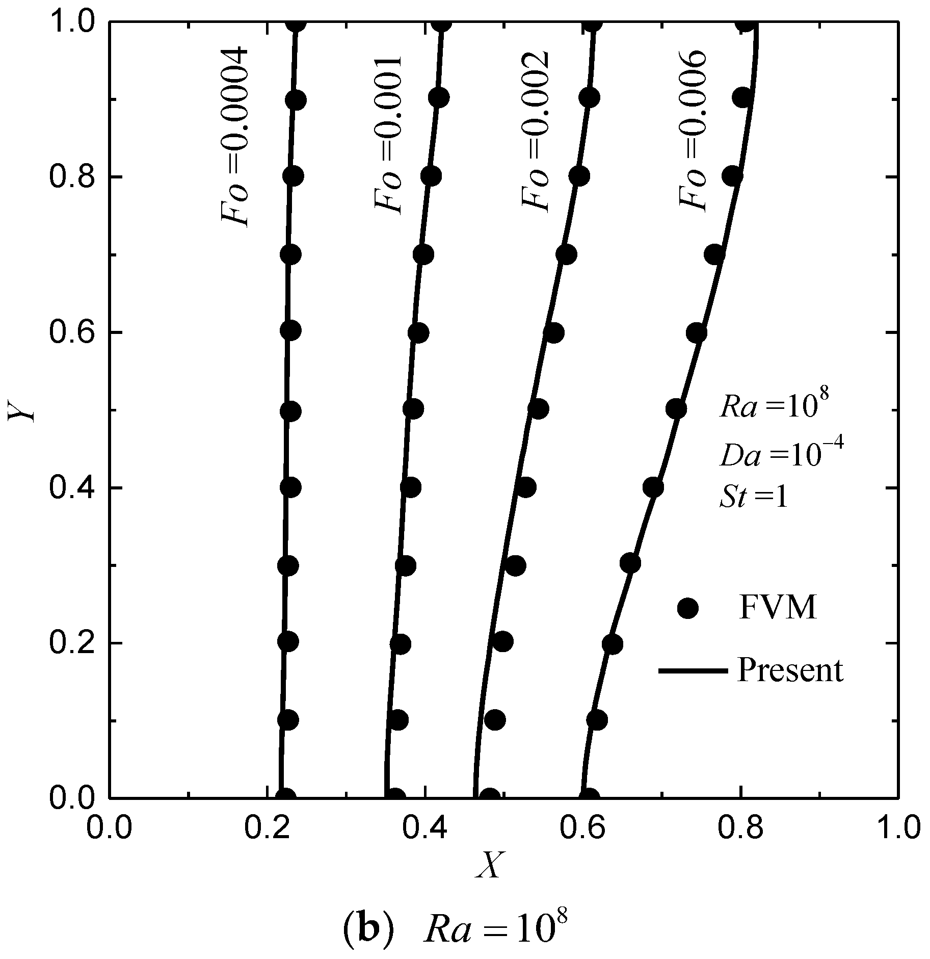
In Figure 2, the melting front at different values of for and 108 with , and are presented. For comparison purpose, the other parameters are chosen as , , , and () [9]. For , is employed, and for , is employed. From the figure it can be found that the CLB results match well with the results obtained by FVM [9]. As show in Figure 2a, at , the shape of the melting front is almost planar since the heat transfer inside the cavity is controlled by conduction due to the large value of metal foam-to-PCM thermal conductivity ratio. As increases (), the effect of natural convection becomes stronger, then the melting front moves faster near the top wall (see Figure 2b).
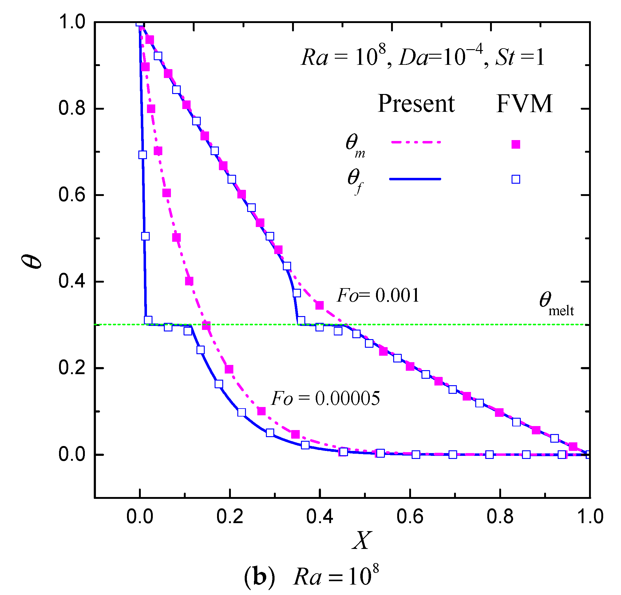
In Figure 3, the temperature profiles (at ) at different values of for and with , and are shown. As can be seen from the figure, at the very beginning (), the thermal non-equilibrium effect is apparent (the temperature difference is very high). As increases, the temperature difference progressively decreases due to the interfacial heat transfer. At , the temperature difference tends to except in the mushy zone, indicating that the thermal non-equilibrium effect at this stage is weak. As clearly illustrated in Figure 3, the temperature difference has a maximum value near the phase-change region (mushy zone). The FVM results [9] are also shown in Figure 3 for comparisons. It can be found that the CLB results are in good agreement with those results in Ref. [9].
The flow field with the phase field at different values of for with , and are presented in Figure 4. As shown in the figure, an elliptical shape vortex appears in the liquid region at . As increases, natural convection effect becomes stronger, resulting in more hot liquid to move upwards, and consequently, the PCM melts faster in the upper region of the cavity. Although the Rayleigh number is high, the natural convection effect is weak since it has been severely suppressed by the effect caused by the metal foam’s ligament, and, during the melting process, the heat conduction through the high thermal conductive metal foam dominates the heat transfer.
Since the cascaded collision model has tunable relaxation parameters as well as a high degree of Galilean invariance, it is expected that the unphysical numerical diffusion can be effectively eliminated in numerical simulations by using the CLB model. To confirm this statement, the liquid fraction distributions calculated by the CLB and BGK-LB models at for with , and are presented in Figure 5. The BGK-LB result means that the PCM’s temperature field is solved by the enthalpy-based BGK-LB equation (when is an identity matrix and , the enthalpy-based CLB equation degrades into the enthalpy-based BGK-LB equation with ). As can be seen in Figure 5a, the liquid fraction distribution calculated by the BGK-LB model exhibits significant numerical oscillations because the BGK-LB model has no free relaxation parameters to eliminate the effect of numerical diffusion on numerical simulations. On the contrary, the effect of numerical diffusion is almost invisible in Figure 5b because the CLB model has free relaxation parameters to eliminate such an effect. By setting , the effect of the numerical diffusion on numerical simulations can be effectively eliminated by the present CLB model.
and are functions of the structure of the porous media. Equation (6) is proposed for packed beds of spherical particles based on Ergun’s experimental study, while Equation (7) is proposed for high porosity metal foams such as aluminum foam [33,34]. In what follows, the empirical correlations for and given by Equations (6) and (7) are evaluated. In numerical simulations, the related parameters are set as , . Numerical simulations are conducted based on . The total liquid fractions for different porosities with and are presented in Figure 6. For a low value of porosity (), the total liquid fraction predicted with Equation (6) is almost the same as that predicted with Equation (7). As the porosity increases, the two empirical correlations yield different results (see Figure 6b–d). When and are given by Equation (6), the melting rate of the PCM is faster than that predicted with Equation (7). This can be expected because the permeability given by Equation (6) is much larger than that given by Equation (7) at high porosities, leading to a stronger convection effect which promotes the heat transfer during melting process. Hence, for high porosity metal foams, appropriate empirical correlations should be employed. Since Equation (6) is proposed for packed beds, it overestimates the melting rate of the PCM. The empirical correlations given by Equation (7) are expected to provide a good estimate of the practical situations.
In Figure 7, the total liquid fractions of and for different porosities with and given by Equation (7) are shown. As can be seen in the figure, when increases, the PCM’s melting rate decreases. An increase in the metal foam’s porosity leads to stronger convection effect of the liquid; however, it also reduces the effect of conduction through the metal foam’s ligament. This observation denotes that the total heat transfer from hot (left) wall is dominated by heat conduction through the high thermal conductive metal foam. The comparison between the total liquid fractions of and indicates that the effect of on melting is weak because the convection has been severely suppressed by the metal foam’s ligament. Although smaller porosity increases the PCM’s melting rate, it also denotes smaller volume of PCM for LHS. A further optimization investigation on porosity of the metal foam to balance the PCM’s melting rate and LHS capacity is quite necessary.
5. Conclusions
An enthalpy-based CLB model is constructed for investigating heat transfer in solid-liquid PCMs with metal foams. The effects of the inertial coefficient, permeability and porosity on phase-change processes are examined. The findings of this research are:
- (1)
- The melting front and temperature profiles at different Fourier numbers predicted by the CLB model match well with the available data in previous studies, demonstrating the effectiveness and practicability of the CLB model for investigating heat transfer in solid-liquid PCMs with metal foams.
- (2)
- The empirical correlations of and given by Equation (6) based on packed beds overestimate the PCM’s melting rate when the metal foam’s porosity is high, while the empirical correlations for metal foams such as aluminum foam given by Equation (7) are expected to provide a good estimate of the practical situations.
- (3)
- The PCM’s melting rate increases as the metal foam’s porosity decreases since the total heat transfer from the hot wall is dominated by heat conduction through high thermal conductive metal foam. Moreover, the effect of the Rayleigh number on phase-change process is weak since it has been severely suppressed by the metal foam’s ligament.
- (4)
- Although smaller porosity increases the PCM’s melting rate, it also reduces the volume of PCM for LHS, leading to a lower LHS capability. A further optimization investigation on metal foam’s porosity to balance PCM’s melting rate and LHS capacity is quite necessary.
Author Contributions
Conceptualization, X.-B.F. and Q.L.; methodology, X.-B.F.; software, X.-B.F.; validation, X.-B.F.; revision, X.-B.F. and Q.L.; investigation, X.-B.F.; supervision, Q.L. All authors have read and agreed to the published version of the manuscript.
Funding
This research was funded by the Natural Science Foundation of Shaanxi Province (Nos. 2021JM-355 and 2020JQ-919).
Acknowledgments
The authors are grateful to the anonymous referees, who improved the quality of the manuscript with their comments.
Conflicts of Interest
The authors declare no conflict of interest.
Nomenclature
| heat capacity ratio (metal foam-to-PCM) | |
| lattice speed, | |
| sound speed, | |
| sound speed, | |
| temperature | |
| gravitational acceleration | |
| mean particle diameter or mean diameter of the pores | |
| pressure | |
| fiber diameter of metal foam | |
| Darcy number | |
| discrete lattice velocity | |
| total body force | |
| characteristic length | |
| total liquid fraction | |
| Fourier number | |
| G | buoyancy force |
| effective thermal conductivity (metal foam) | |
| volumetric heat transfer coefficient | |
| viscosity ratio | |
| transformation matrix | |
| shift matrix | |
| Rayleigh number | |
| Stefan number | |
| reference temperature | |
| hot wall’ temperature | |
| thermal conductivity ratio (metal foam-to-PCM) | |
| cold wall’s temperature | |
| initial temperature | |
| melting temperature | |
| thermal conductivity (PCM) | |
| velocity | |
| , | coordinates, , |
| specific heat | |
| thermal dispersion conductivity | |
| specific surface area | |
| effective thermal conductivity (PCM) | |
| interfacial heat transfer coefficient | |
| liquid fraction | |
| latent heat | |
| inertial coefficient | |
| permeability | |
| Prandtl number | |
| Thermal diffusivity (liquid PCM) | |
| effective thermal diffusivity (fluid) | |
| effective thermal diffusivity (metal foam) | |
| thermal expansion coefficient | |
| density | |
| porosity of metal foam | |
| ve | effective kinematic viscosity |
| kinematic viscosity (liquid PCM) | |
| , | model parameters |
| km | thermal conductivity (metal foam) |
| lattice spacing | |
| time step | |
| thermal diffusivity ratio (metal foam-to-PCM) | |
| Subscripts | |
| fluid (PCM) | |
| metal foam | |
| liquid PCM | |
| solid PCM | |
References
- Zalba, B.; Marίn, J.M.; Cabeza, L.F.; Mehling, H. Review on thermal energy storage with phase change: Materials, heat transfer analysis and applications. Appl. Therm. Eng. 2003, 23, 251–283. [Google Scholar] [CrossRef]
- Sharma, A.; Tyagi, V.V.; Chen, C.R.; Buddhi, D. Review on thermal energy storage with phase change materials and applications. Renew. Sustain. Energy Rev. 2009, 13, 318–345. [Google Scholar] [CrossRef]
- Miansari, M.; Nazari, M.; Toghraie, D.; Akbari, O.A. Investigating the thermal energy storage inside a double-wall tank utilizing phase-change materials (PCMs). J. Therm. Anal. Calorim. 2019, 139, 2283–2294. [Google Scholar] [CrossRef]
- Yan, S.; Fazilati, M.A.; Toghraie, D.; Khalili, M.; Karimipour, A. Energy cost and efficiency analysis of greenhouse heating system enhancement using phase change material: An experimental study. Renew. Energy 2021, 170, 133–140. [Google Scholar] [CrossRef]
- Pielichowska, K.; Pielichowski, K. Phase change materials for thermal energy storage. Prog. Mater. Sci. 2014, 65, 67–123. [Google Scholar] [CrossRef]
- Tao, Y.B.; He, Y.-L. A review of phase change material and performance enhancement method for latent heat storage system. Renew. Sustain. Energy Rev. 2018, 93, 245–259. [Google Scholar] [CrossRef]
- Liu, L.; Su, D.; Tang, Y.; Fang, G. Thermal conductivity enhancement of phase change materials for thermal energy storage: A review. Renew. Sustain. Energy Rev. 2016, 62, 305–317. [Google Scholar] [CrossRef]
- Zhao, Y.; Zhao, C.; Xu, Z.; Xu, H. Modeling metal foam enhanced phase change heat transfer in thermal energy storage by using phase field method. Int. J. Heat Mass Transf. 2016, 99, 170–181. [Google Scholar] [CrossRef]
- Krishnan, S.; Murthy, J.Y.; Garimella, S.V. A two-temperature model for solid-liquid phase change in metal foams. J. Heat Transf. 2004, 127, 995–1004. [Google Scholar] [CrossRef] [Green Version]
- McNamara, G.R.; Zanetti, G. Use of the boltzmann equation to simulate lattice-gas automata. Phys. Rev. Lett. 1988, 61, 2332–2335. [Google Scholar] [CrossRef] [PubMed]
- Frisch, U.; Hasslacher, B.; Pomeau, Y. Lattice-Gas automata for the navier-stokes equation. Phys. Rev. Lett. 1986, 56, 1505–1508. [Google Scholar] [CrossRef] [Green Version]
- He, Y.-L.; Liu, Q.; Tao, W.-Q. Lattice Boltzmann methods for single-phase and solid-liquid phase-change heat transfer in porous media: A review. Int. J. Heat Mass Transf. 2018, 129, 160–197. [Google Scholar] [CrossRef] [Green Version]
- Chen, S.; Doolen, G.D. Lattice Boltzmann method for fluid flows. Annu. Rev. Fluid Mech. 1998, 30, 329–364. [Google Scholar] [CrossRef] [Green Version]
- Li, Q.; Luo, K.; Kang, Q.; He, Y.; Chen, Q. Lattice Boltzmann methods for multiphase flow and phase-change heat transfer. Prog. Energy Combust. Sci. 2015, 52, 62–105. [Google Scholar] [CrossRef] [Green Version]
- De Fabritiis, G.; Mancini, A.; Mansutti, D.; Succi, S. Mesoscopic models of liquid/solid phase transitions. Int. J. Mod. Phys. C 1998, 9, 1405–1415. [Google Scholar] [CrossRef]
- Miller, W.; Succi, S.; Mansutti, D. Lattice Boltzmann model for anisotropic liquid-solid phase transition. Phys. Rev. Lett. 2001, 86, 3578–3581. [Google Scholar] [CrossRef] [PubMed]
- Miller, W.; Rasin, I.; Succi, S. Lattice Boltzmann phase-field modelling of binary-alloy solidification. Phys. A Stat. Mech. Its Appl. 2006, 362, 78–83. [Google Scholar] [CrossRef]
- Jiaung, W.S.; Ho, J.R.; Kuo, C.P. Lattice Boltzmann method for the heat conduction problem with phase change. Numer. Heat Transf. B 2001, 39, 167–187. [Google Scholar]
- Huang, R.; Wu, H.; Cheng, P. A new lattice Boltzmann model for solid–liquid phase change. Int. J. Heat Mass Transf. 2013, 59, 295–301. [Google Scholar] [CrossRef]
- Huang, R.; Wu, H. Phase interface effects in the total enthalpy-based lattice Boltzmann model for solid–liquid phase change. J. Comput. Phys. 2015, 294, 346–362. [Google Scholar] [CrossRef]
- Huang, R.; Wu, H. An immersed boundary-thermal lattice Boltzmann method for solid–liquid phase change. J. Comput. Phys. 2014, 277, 305–319. [Google Scholar] [CrossRef]
- Li, Z.; Yang, M.; Zhang, Y. Numerical simulation of melting problems using the Lattice Boltzmann method with the interfacial tracking method. Numer. Heat Transf. Part A Appl. 2015, 68, 1175–1197. [Google Scholar] [CrossRef]
- Gao, D.; Chen, Z.; Shi, M.; Wu, Z. Study on the melting process of phase change materials in metal foams using lattice Boltzmann method. Sci. China Ser. E Technol. Sci. 2010, 53, 3079–3087. [Google Scholar] [CrossRef]
- Gao, D.; Chen, Z. Lattice Boltzmann simulation of natural convection dominated melting in a rectangular cavity filled with porous media. Int. J. Therm. Sci. 2011, 50, 493–501. [Google Scholar] [CrossRef]
- Jourabian, M.; Darzi, A.A.R.; Akbari, O.A.; Toghraie, D. The enthalpy-based lattice Boltzmann method (LBM) for simulation of NePCM melting in inclined elliptical annulus. Phys. A Stat. Mech. Its Appl. 2019, 548, 123887. [Google Scholar] [CrossRef]
- Liu, Q.; He, Y.-L. Double multiple-relaxation-time lattice Boltzmann model for solid–liquid phase change with natural convection in porous media. Phys. A Stat. Mech. its Appl. 2015, 438, 94–106. [Google Scholar] [CrossRef] [Green Version]
- Liu, Q.; He, Y.-L. Enthalpy-based multiple-relaxation-time Lattice Boltzmann method for solid-liquid phase-change heat transfer in metal foams. Phys. Rev. E 2017, 96, 023303. [Google Scholar] [CrossRef] [PubMed] [Green Version]
- Gao, D.; Chen, Z.; Zhang, D.; Chen, L. Lattice Boltzmann modeling of melting of phase change materials in porous media with conducting fins. Appl. Therm. Eng. 2017, 118, 315–327. [Google Scholar] [CrossRef]
- Geier, M.; Greiner, A.; Korvink, J.G. Cascaded digital Lattice Boltzmann automata for high Reynolds number flow. Phys. Rev. E 2006, 73, 066705. [Google Scholar] [CrossRef]
- Fei, L.; Luo, K.H.; Lin, C.; Li, Q. Modeling incompressible thermal flows using a central-moments-based Lattice Boltzmann method. Int. J. Heat Mass Transf. 2018, 120, 624–634. [Google Scholar] [CrossRef]
- Liu, Q.; Feng, X.-B. Numerical modelling of microchannel gas flows in the transition flow regime using the cascaded Lattice Boltzmann method. Entropy 2019, 22, 41. [Google Scholar] [CrossRef] [Green Version]
- Feng, X.-B.; Liu, Q.; He, Y.-L. Numerical simulations of convection heat transfer in porous media using a cascaded lattice Boltzmann method. Int. J. Heat Mass Transf. 2020, 151, 119410. [Google Scholar] [CrossRef]
- Calmidi, V.V. Transport Phenomena in High Porosity Fibrous Metal Foams; University of Colorado: Boulder, CO, USA, 1998. [Google Scholar]
- Calmidi, V.V.; Mahajan, R.L. Forced convection in high porosity metal foams. J. Heat Transf. 2000, 122, 557–565. [Google Scholar] [CrossRef]
- Churchill, S.W.; Chu, H.H. Correlating equations for laminar and turbulent free convection from a horizontal cylinder. Int. J. Heat Mass Transf. 1975, 18, 1049–1053. [Google Scholar] [CrossRef]
- Huang, R.; Wu, H. Total enthalpy-based Lattice Boltzmann method with adaptive mesh refinement for solid-liquid phase change. J. Comput. Phys. 2016, 315, 65–83. [Google Scholar] [CrossRef]
- Guo, Z.L.; Zheng, C.G.; Shi, B.C. Non-equilibrium extrapolation method for velocity and pressure boundary conditions in the lattice Boltzmann method. Chin. Phys. 2002, 11, 366. [Google Scholar]
Figure 1.
Schematic of melting with natural convection in metal foams.

Figure 2.
The melting front () at different values of for and with , and . (lines: present; symbols: FVM results [9]).
Figure 2.
The melting front () at different values of for and with , and . (lines: present; symbols: FVM results [9]).


Figure 3.
Temperature profiles at the mid-height of the cavity () at different values of for and with , and . (lines: present; symbols: FVM results [9]).
Figure 3.
Temperature profiles at the mid-height of the cavity () at different values of for and with , and . (lines: present; symbols: FVM results [9]).


Figure 4.
Streamlines with the phase field at different values of for with , and .


Figure 5.
Local enlargement view of the liquid fraction distributions calculated by the BGK-LB and CLB models at for with , and .
Figure 5.
Local enlargement view of the liquid fraction distributions calculated by the BGK-LB and CLB models at for with , and .


Figure 6.
The total liquid fractions for different porosities with and .

Figure 7.
The total liquid fractions for different porosities with and given by Equation (7).

Publisher’s Note: MDPI stays neutral with regard to jurisdictional claims in published maps and institutional affiliations. |
© 2022 by the authors. Licensee MDPI, Basel, Switzerland. This article is an open access article distributed under the terms and conditions of the Creative Commons Attribution (CC BY) license (https://creativecommons.org/licenses/by/4.0/).
Share and Cite
MDPI and ACS Style
Feng, X.-B.; Liu, Q. Simulating Solid-Liquid Phase-Change Heat Transfer in Metal Foams via a Cascaded Lattice Boltzmann Model. Entropy 2022, 24, 307. https://0-doi-org.brum.beds.ac.uk/10.3390/e24030307
AMA Style
Feng X-B, Liu Q. Simulating Solid-Liquid Phase-Change Heat Transfer in Metal Foams via a Cascaded Lattice Boltzmann Model. Entropy. 2022; 24(3):307. https://0-doi-org.brum.beds.ac.uk/10.3390/e24030307
Chicago/Turabian StyleFeng, Xiang-Bo, and Qing Liu. 2022. "Simulating Solid-Liquid Phase-Change Heat Transfer in Metal Foams via a Cascaded Lattice Boltzmann Model" Entropy 24, no. 3: 307. https://0-doi-org.brum.beds.ac.uk/10.3390/e24030307
Note that from the first issue of 2016, this journal uses article numbers instead of page numbers. See further details here.