
Finite-Time H∞ Controllers Design for Stochastic Time-Delay Markovian Jump Systems with Partly Unknown Transition Probabilities


1
College of Mathematics and Systems Science, Shandong University of Science and Technology, Qingdao 266590, China
2
Department of Fundamental Courses, Shandong University of Science and Technology, Jinan 250031, China
3
Department of Electrical Engineering and Information Technology, Shandong University of Science and Technology, Jinan 250031, China
*
Authors to whom correspondence should be addressed.
†
These authors contributed equally to this work.
Entropy 2024, 26(4), 292; https://0-doi-org.brum.beds.ac.uk/10.3390/e26040292
Submission received: 28 January 2024
/
Revised: 22 March 2024
/
Accepted: 23 March 2024
/
Published: 27 March 2024
Abstract
:This paper concentrates on the finite-time control problem for a type of stochastic discrete-time Markovian jump systems, characterized by time-delay and partly unknown transition probabilities. Initially, a stochastic finite-time (SFT) state feedback controller and an SFT observer-based state feedback controller are constructed to realize the closed-loop control of systems. Then, based on the Lyapunov–Krasovskii functional (LKF) method, some sufficient conditions are established to guarantee that closed-loop systems (CLSs) satisfy SFT boundedness and SFT boundedness. Furthermore, the controller gains are obtained with the use of the linear matrix inequality (LMI) approach. In the end, numerical examples reveal the reasonableness and effectiveness of the proposed designing schemes.
1. Introduction
The structure or parameters of various practical systems often undergoes changes due to environmental mutations, component failures, and other factors, resulting in a decrease in system performance and potential instability [1]. How to ensure the stability of mutation systems has been one of the hot topics for scholars. Markovian jump systems (MJSs), a type of hybrid systems consisting of several subsystems, can be used to model dynamical systems with structural mutations and have been extensively researched in both the practical and theoretical domains [2,3]. An adaptive neural network-based control approach was devised in [4] to address the problem of fault-tolerant control for nonlinear MJSs. In [5], the asynchronous filtering problem of MJSs affected by time-varying and infinite distributed delays was studied by using the homogeneous polynomial method. For stochastic T-S fuzzy singular MJSs, the robust sliding mode control problem was studied in [6,7]. The authors of [8] studied the fault-detection filter design problem of uncertain singular MJSs by means of the LKF and convex polyhedron techniques. In addition, for the achievements regarding the stability and stabilization of MJSs, readers may see [9,10] and references therein.
It should be emphasized that there is a qualification in references [4,5,6,7,8,9,10], that is, the transition probability (TP) information of MJSs must be exactly and completely known. However, due to the limitations of measurement costs and measuring instruments, this condition is difficult to meet in the actual system modeling. As a result, it is essential and significant to investigate MJSs with partly unknown TPs [11]. For networked MJSs with partly unknown TPs, the event-triggered dynamic output feedback control problem and sliding mode control problem were solved in [12,13], respectively. For a type of singular MJSs with partly unknown TPs, the filtering problem was studied in [14,15]. The authors of [16] achieved the event-triggered guaranteed cost control for time-delay MJSs with partly unknown TPs, and some sufficient conditions were established to guarantee the presence of guaranteed cost controllers. In [17], a state feedback controller was constructed to ensure that MJSs with partly unknown TPs were stochastic stable. A sliding mode controller based on an adaptive neural network was proposed in [18], and the reliable control problem of uncertain MJSs with partially unknown TPs was studied.
Notably, most of the above research findings mainly concentrate on the asymptotic behavior of systems in an infinite-time interval, namely, as in the Lyapunov stability theory. However, in many practical systems, such as vehicle emergency braking systems [19], aircraft-tracking systems [20], and ship-maneuvering systems [21], it is required that the systems respond ideally to work in a finite time interval. To realize this practical need, in 1961, Dorato proposed finite-time stability [22]. Since finite-time stability has a better transient performance, a faster response speed, and a higher tracking accuracy, it has been applied to MJSs [23,24,25,26], T-S fuzzy systems [27,28,29], nonlinear pulse systems [30,31], mean-field systems [32,33,34], and so on.
In addition to requiring better transient performance, modern industries increasingly emphasize the anti-interference performance of control systems. Both external disturbances and imprecise modeling can adversely affect the performance of control systems. To weaken the effect of external disturbances, control has emerged. Recently, many scholars have carried out plenty of research on finite-time control [35,36,37,38,39,40,41]. Specifically, ref. [35] introduced a new switching dynamic event-triggering mechanism, and discussed the finite-time control problem for switching fuzzy systems. In [36], the finite-time control problem of nonlinear pulse switching systems was studied to guarantee that the CLS was bounded. On the other hand, due to the constraints of measurement technology and measurement costs, the system state information is frequently challenging to measure directly. In tackling this challenge, many meaningful results of finite-time observer-based controller designing schemes have been successfully attained; see [37,38,39,40,41] and references therein.
At present, the study of continuous-time MJSs has obtained rich results. With the popularization of digital controllers and the development of computer science and technology, the research on discrete-time systems has attracted much attention. Discrete-time MJSs provide a framework for modeling and analyzing a variety of complex systems in the real world [42]. Through the discrete description of the system, it is easier to analyze the dynamic behavior, stability, and convergence of the system [43]. This kind of modeling and analysis is essential for understanding and predicting the behavior of systems [44], and is widely used in control systems.
Inspired by the preceding analysis, this article presents the designing schemes of a stochastic finite-time state feedback controller and a stochastic finite-time observer-based state feedback controller for a discrete-time MJS. Different from [17,38], the MJS considered in this paper is influenced by a time delay and stochastic white noise, which is more in line with the actual demand, but also increases the difficulty of the article derivation. Compared with the existing literature, the primary contributions of this study include the following:
(I) In this paper, the state feedback control strategy and the observer-based state feedback control strategy are adopted. The concepts of SFT state feedback stabilization and SFT observer-based state feedback stabilization for time-delay MJSs are defined simultaneously for the first time. The results of [17,38,44] are extended to time-delay MJSs with partially unknown TPs.
(II) By constructing a delay-dependent LKF, several sufficient conditions are given to ensure that the CLS is SFT -bounded under two control strategies.
The article is structured as follows: Section 2 presents an introduction to the system along with some preliminary knowledge. In Section 3, a state feedback controller is designed, and some sufficient conditions for the MJS to be SFT state feedback stabilization are obtained through the LKF and LMI methods. Similar to Section 3, in Section 4 we design an observer-based state feedback controller and verify that the MJS is SFT observer-based state feedback stabilization. In Section 5, the feasibility and effectiveness of this work are validated through two simulation examples. Section 6 summarizes the entire article and provides an outlook on future research directions.
Notation: and represent the matrix inverse and transpose of matrix A, respectively. The expression for a real positive definite matrix A is denoted as . is the block diagonal matrix with on the diagonal. We denote as the identity matrix with dimensions. is the set of positive integers and is the real number set. and are the m-dimensional Euclidean space with 2-norm and the vector space of all matrices with entries in , respectively. represents the mathematical expectation of . The symbol ∗ implies the symmetric hidden matrix entries. This paper presupposes that every specified matrix possesses the necessary dimensions. For ease of understanding, the acronyms in this paper and their corresponding meanings are shown in Table 1.
2. System Description and Preliminary Knowledge
Consider an MJS with a time delay, as outlined below:
where is the system state, is the measured output, is the control output, and is the control input. are the initial conditions. is a positive integer that signifies the fixed time delay. The sequence denotes one-dimensional white noises on the complete probability space , and satisfies and , where is the Kronecker delta. stands for the external disturbance, which satisfies the following:
, , , , , , , , , , , , , and are coefficient matrices with appropriate dimensions. These matrices depend upon the Markovian jump process , which is a discrete-time, discrete-state Markovian chain taking values in a finite state space with transition probabilities , where , denotes the transition probability from mode i at time k to mode j at time , and satisfies . When , the system parameter matrices are expressed by , , , , , , and so on. In addition, and are independent of each other.
In this paper, it is presumed that the information in the TP matrix is partially available. In this situation, the TP matrix for an MJS with N modes may be represented by:
where is the unknown TP, for all , and the set S is defined as , where:
Moreover, when , then it can be described as:
where denotes the g-th known element in the i-th row of the TP matrix . Similarly, when , it can be expressed as follows:
where is the g-th unknown element in the i-th row of the TP matrix .
Remark 1.
Since , there are at least two unknown elements in (3), and if there are unknown elements in a certain row, their quantity is at least two.
Lemma 1.
Definition 1.
(SFT stability)
The MJS (1) with is said to be SFT-stable with respect to , if:
holds for matrix , and given scalars .
Remark 2.
Definition 1 means that if the initial state is bounded, then the state trajectory of the system does not exceed a predetermined boundary in a finite time interval under certain conditions, which is different from asymptotic stability. An asymptotically stable system may not be finite-time stable, if its state trajectory exceeds the given upper bound in a finite-time interval, and vice versa.
3. Finite-Time State Feedback Control
3.1. State Feedback Controller
We design the following state feedback controller for MJS (1):
where is the state feedback controller gain to be designed and is denoted by when . Then, the resulting CLS can be described as follows:
where , , .
Definition 3.
where , , .
(SFT boundedness)
The CLS (9) is said to be SFT -bounded with respect to if the subsequent two conditions hold:
3.2. Main Results
This section will present some sufficient conditions for the existence of a state feedback controller (8) for system (1).
Theorem 1.
The CLS (9) with partly unknown TPs is SFT -bounded with respect to if there exist the scalars and and matrices and for all , satisfying the following:
where , ,
, ,
, ,
, .
Proof.
For the CLS (9), we consider the following LKF:
Then, we compute the following:
Since the TP matrix contains partly accessible information, not all the probabilities are known. Thus, we denote . are the unknown TPs of . Moreover, from , it is obvious that . Supposing that , we can obtain the following:
Thus, we can obtain the following:
Observing that , from (17) we obtain the following:
Together with (12) and (21), it is clear that . This implies that the CLS (9) satisfies SFT boundedness. Next, we demonstrate that the condition (10) holds under the zero initial condition. From (13), we can obtain the following:
Then, we have the following:
Assuming a zero initial condition and recognizing that for all , we have the following:
Noting that , from (24) we obtain the following:
Therefore the closed-loop MJS (9) is SFT -bounded. □
Remark 3.
Theorem 2.
Consider the state feedback controller (8); if there exist scalars and matrices , , and , for all , satisfying the following conditions:
where
,
,
, ,
Proof.
First, we demonstrate the equivalence between condition (26) and condition (11). According to Lemma 1, (26) is equivalent to the following:
Letting . Pre- and post-multiplying (30) by , we can observe that (30) is equivalent to (11) by using Lemma 1.
On the other hand, from Lemma 1, (29) can be expressed as the following inequality:
Therefore, it is easy to observe that (12) holds. This completes the proof. □
Remark 4.
Remark 5.
It can be seen from Theorem 2 that the controller gain depends on and , that in turn depend on the system matrices of mode i. It is necessary to consider the dynamic characteristics of the system in different modes and the transition probabilities between modes to ensure the stability and the controller in each mode.
4. Finite-Time Observer-Based State Feedback Control
4.1. Observer-Based State Feedback Controller
In the presence of a system state that is not fully measurable, the following observer-based state feedback controller is designed:
where is the estimated state and is the estimated output, and and denote the state feedback gain and observer gain to be determined, respectively. The estimated state error is defined as , and . For , the CLS is represented by the following:
where , , ,
, , ,
Definition 5.
where , , .
(SFT boundedness)
The CLS (33) is said to be SFT -bounded with respect to if the following two conditions hold:
Definition 6.
(SFT observer-based state feedback stabilization)
4.2. Main Results
Theorem 3.
The CLS (33) with the partly unknown TPs is SFT -bounded with respect to if there exist the scalars and , matrix , and positive-definite matrices for all , satisfying the following conditions:
where
Proof.
The proof procedure is similar to Theorem 1, and thus will not be reiterated. □
From the above discussion, system (33) is SFT -bounded. Then, the following theorem will develop the observer-based state feedback controller for system (33).
Theorem 4.
The CLS (33) with the partly unknown TPs is SFT -bounded with respect to if there exist the scalars , matrix , positive-definite matrices , nonsingular matrices , and matrices and for all , satisfying the following conditions:
where ,
,
,
,
.
Then, MJS (1) is called SFT observer-based state feedback stabilization, and the controller gain as well as the observer gain are represented as follows:
Proof.
Remark 7.
Addressing condition (38) through the application of the LMI toolbox is a challenging task. As a solution, constraint (38) can be approximated by the following inequality:
where ϖ represents an exceedingly small positive scalar. According to Lemma 1, the above inequality can be formulated as follows:
Remark 8.
We can note that conditions (26), (29), (37), and (41) are not strict LMIs; however, once we fix the parameters α and β, the conditions can be turned into LMI-based feasibility problems. Therefore, the feasibility of the conditions stated in Theorems 2 and 4 can be turned into the following feasibility problems with the fixed parameters α and β, respectively:
5. Numerical Examples
In this section, we present two examples to validate the effectiveness and practicality of the proposed method. The first example is used to show the effectiveness of the state feedback controller (8) design approach developed in Theorem 2 for MJSs (1) with partly unknown transition probabilities.
Example 1.
Consider MJS (1) with three modes, and the coefficient matrices are given as follows:
Mode 1 ():
,
Mode 2 ():
,
Mode 3 ():
,
The partly unknown TP matrix with three modes is given as follows:
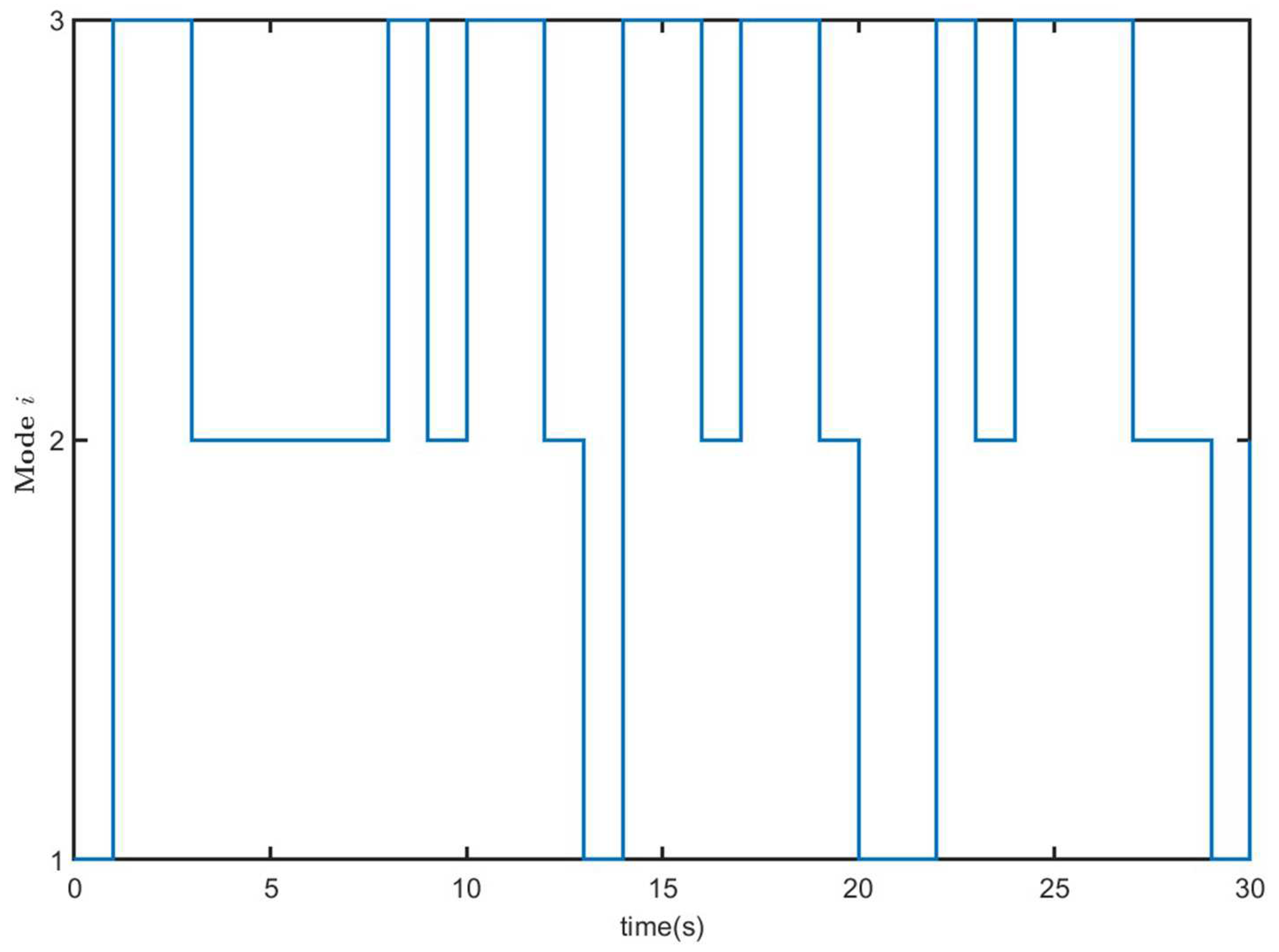
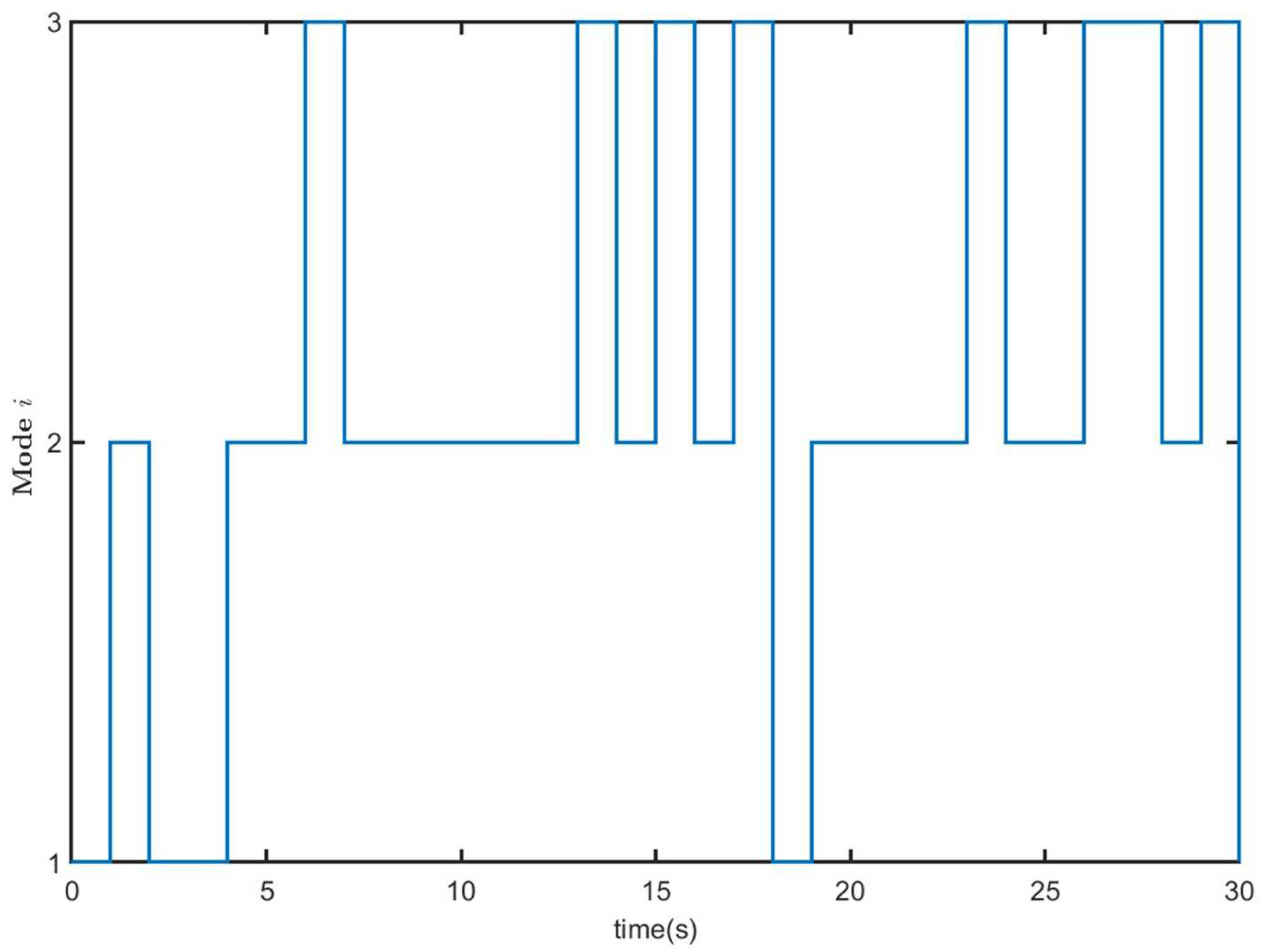
where is the unknown element. One possible mode evolution is given in Figure 1.
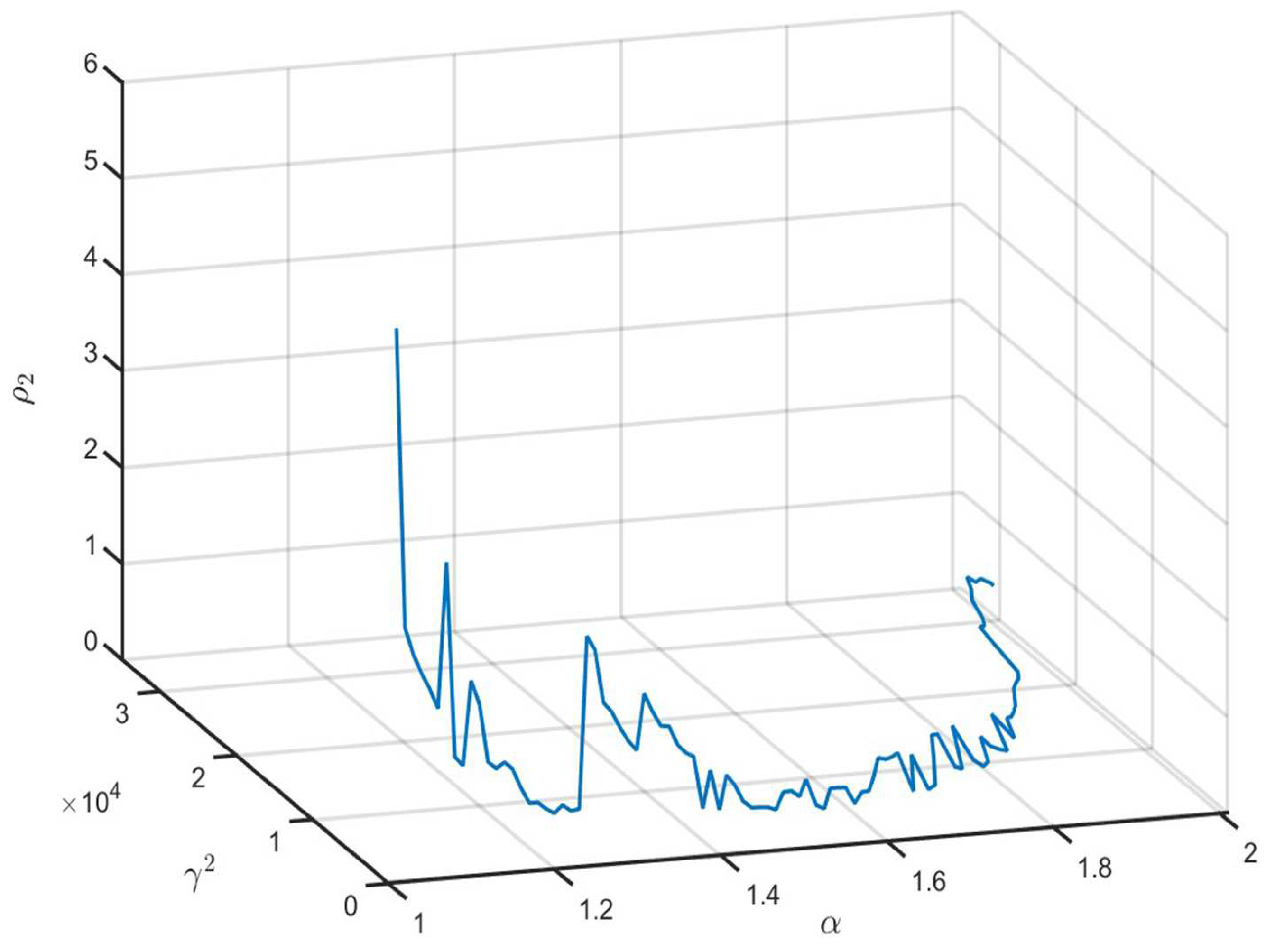
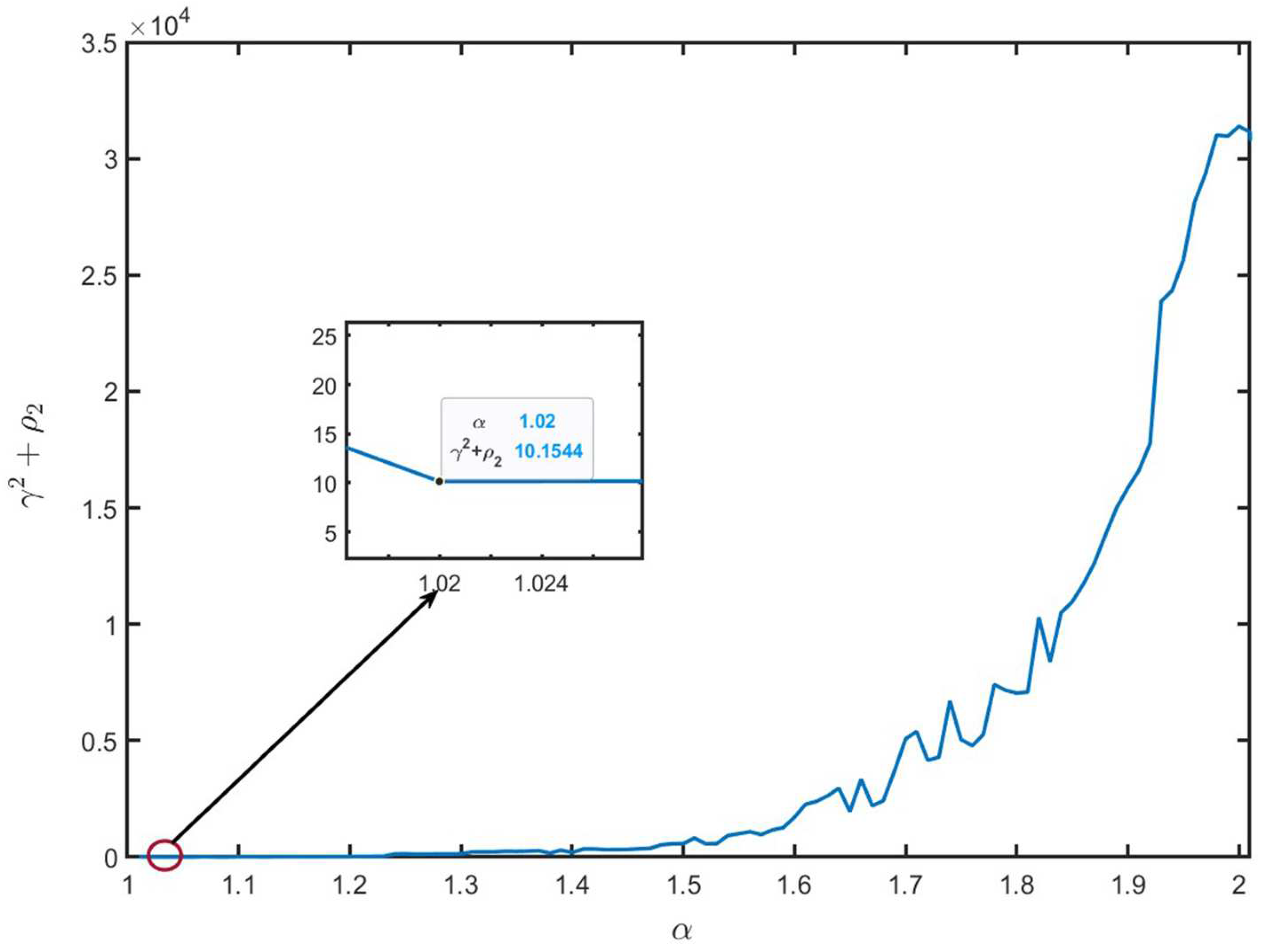
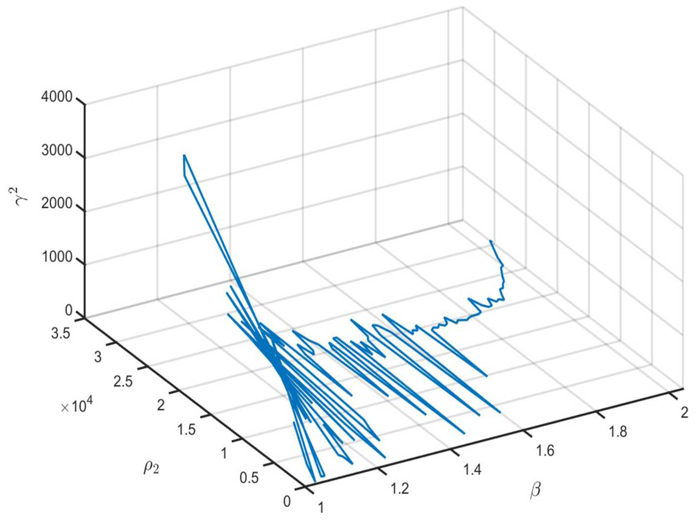
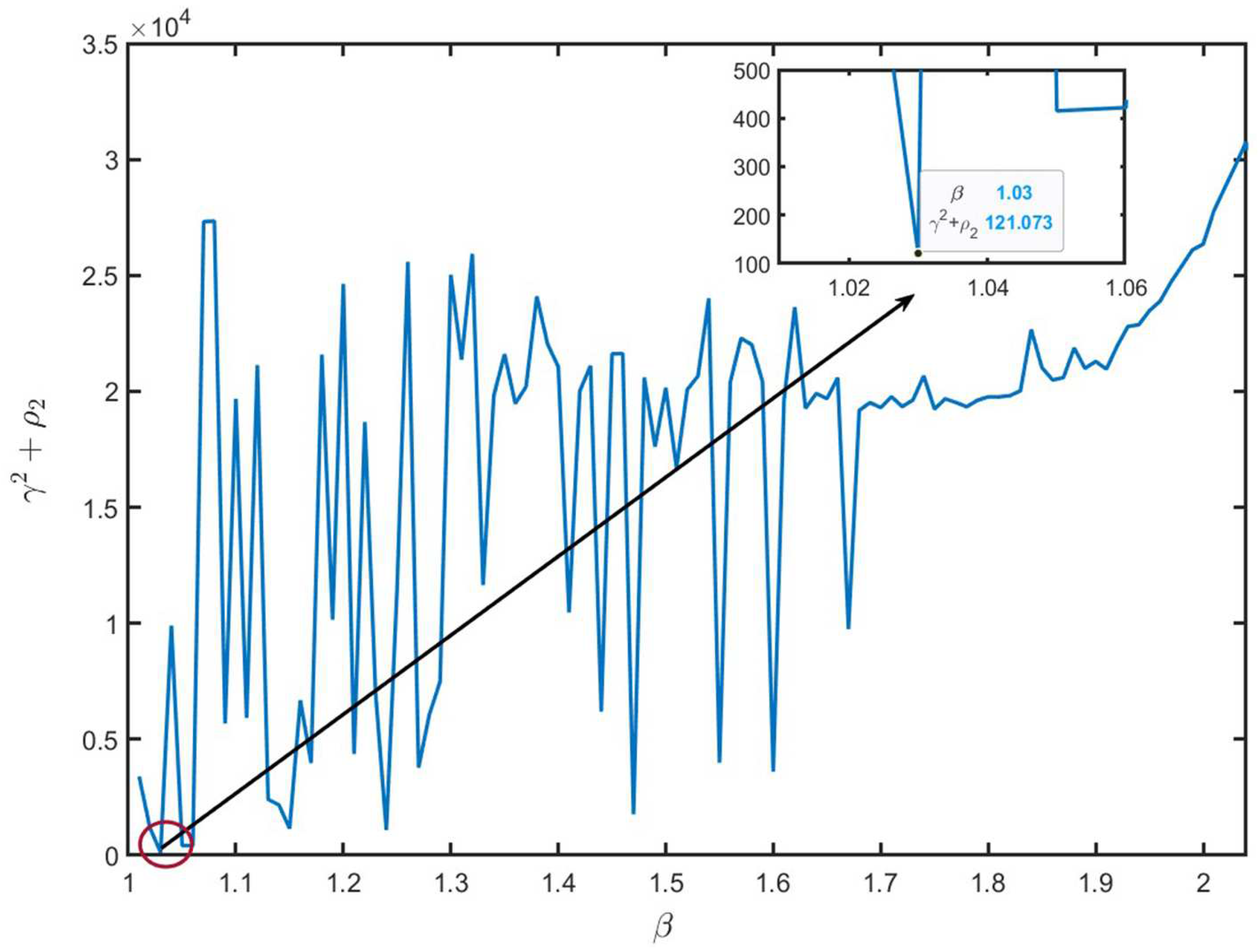
According to Remark 8, the minimum value of relies on the parameter . We can obtain the feasible solution of (45) when . Figure 2 and Figure 3 show the optimal values of , and with different values. We can see that the optimal values , , and when .
Next, letting , and , and solving LMIs (26) to (29), we obtain , , and , and the gains of the state feedback controller (8) are as follows:
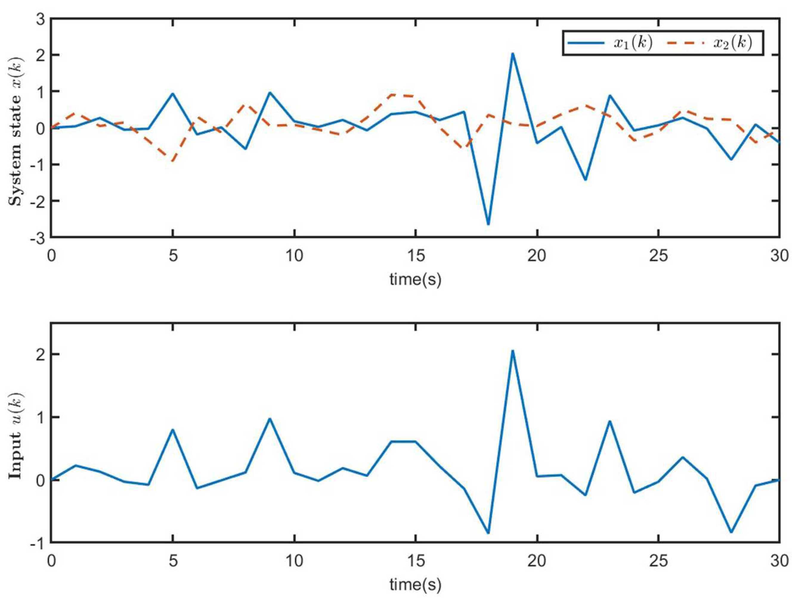
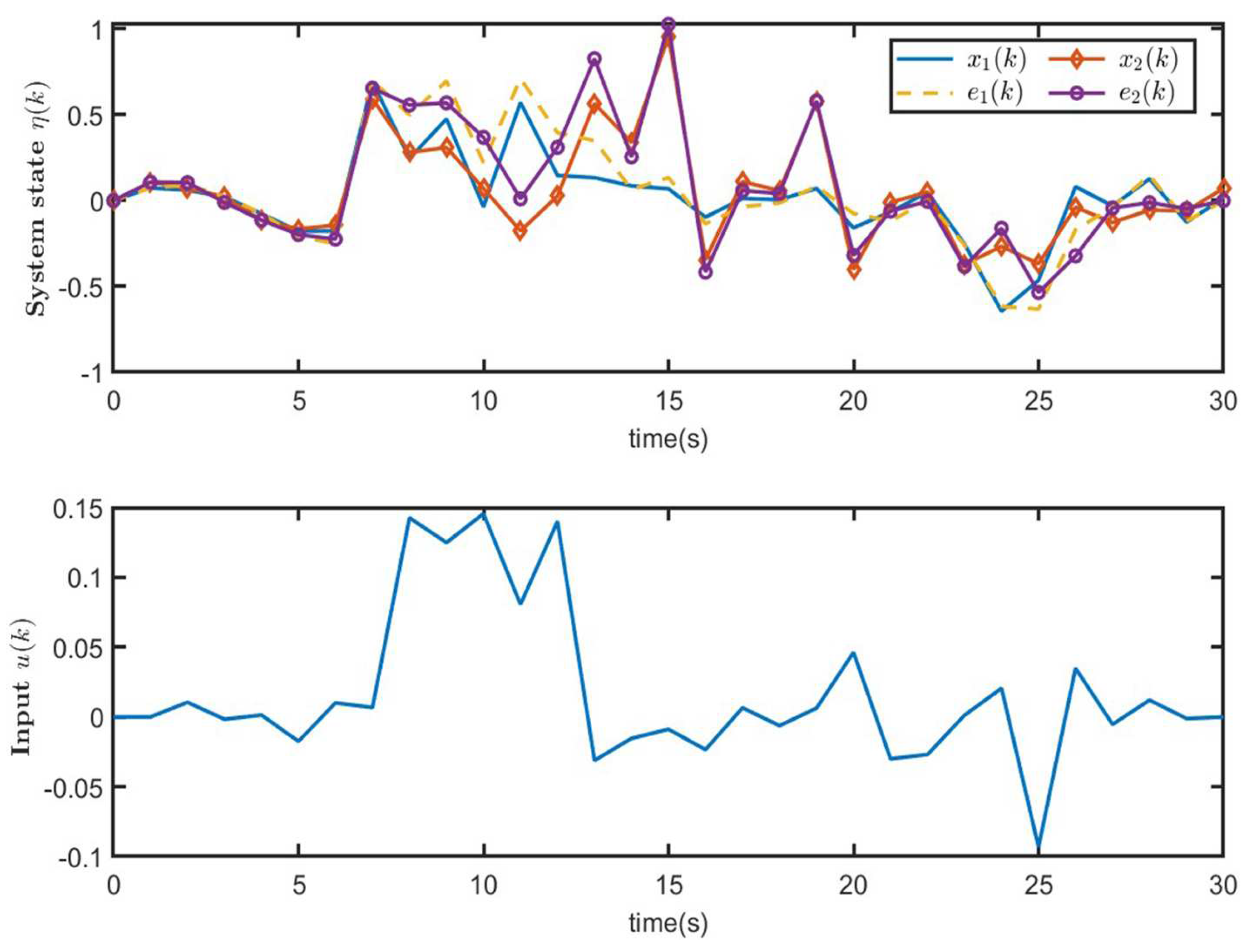
Then, we set the initial value for MJS (1) and CLS (9), and the external disturbance signal , which satisfies .
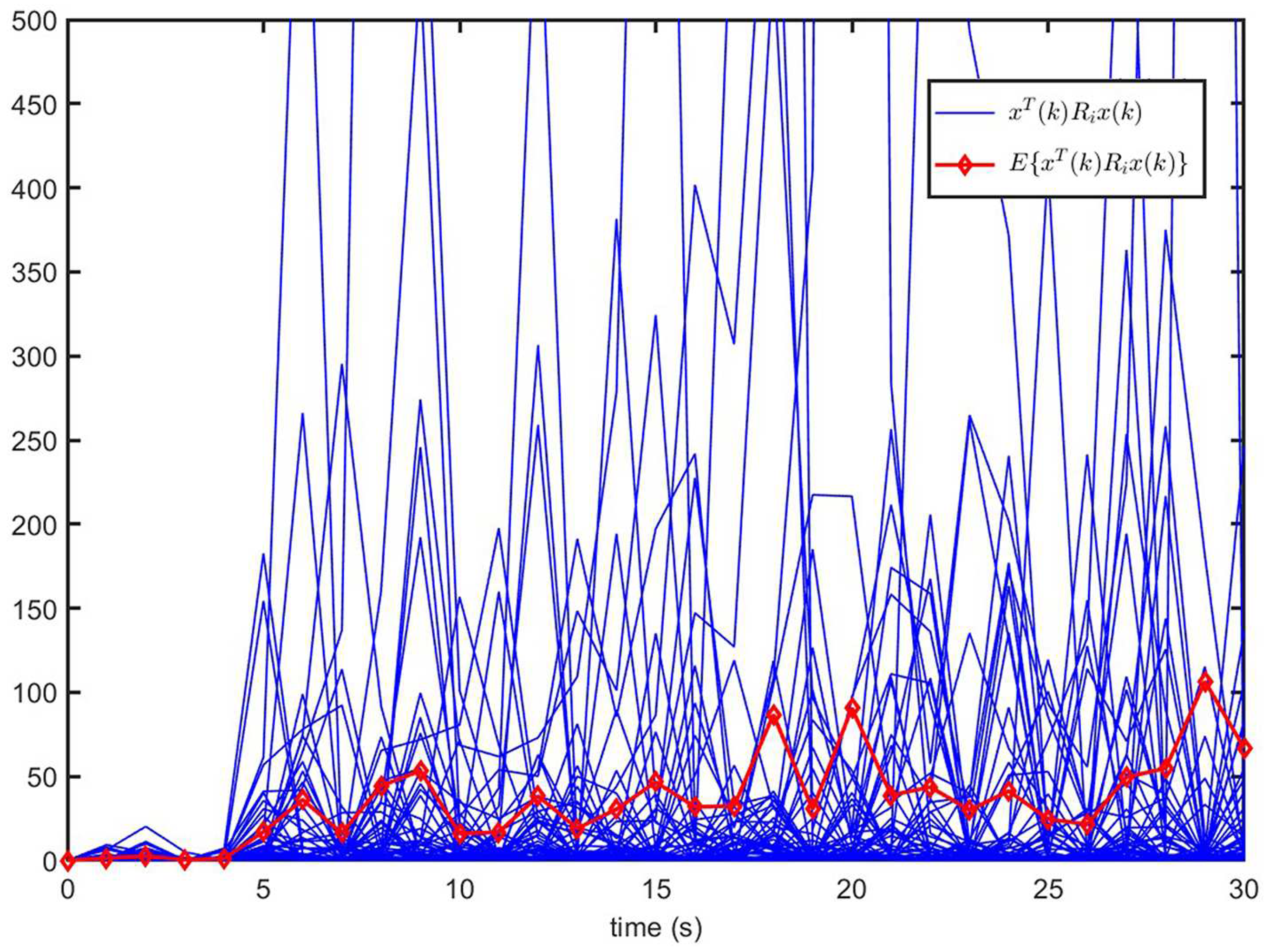
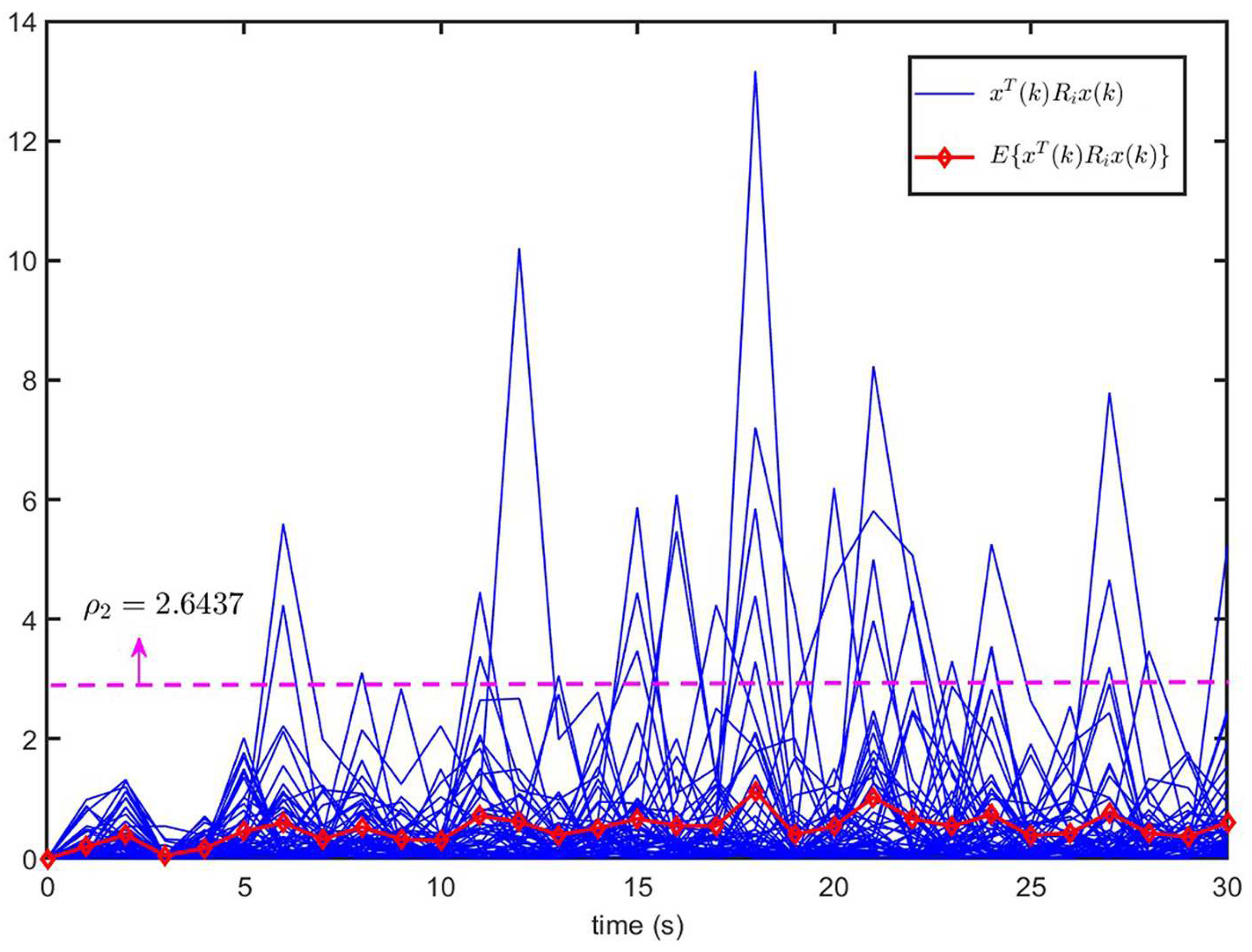
Figure 4 shows the trajectories of (50 curves) and of the open-loop system (1) (). It can be seen that the trajectory of exceeds the upper bound , despite . This implies that the open-loop system (1) is not finite-time bound.
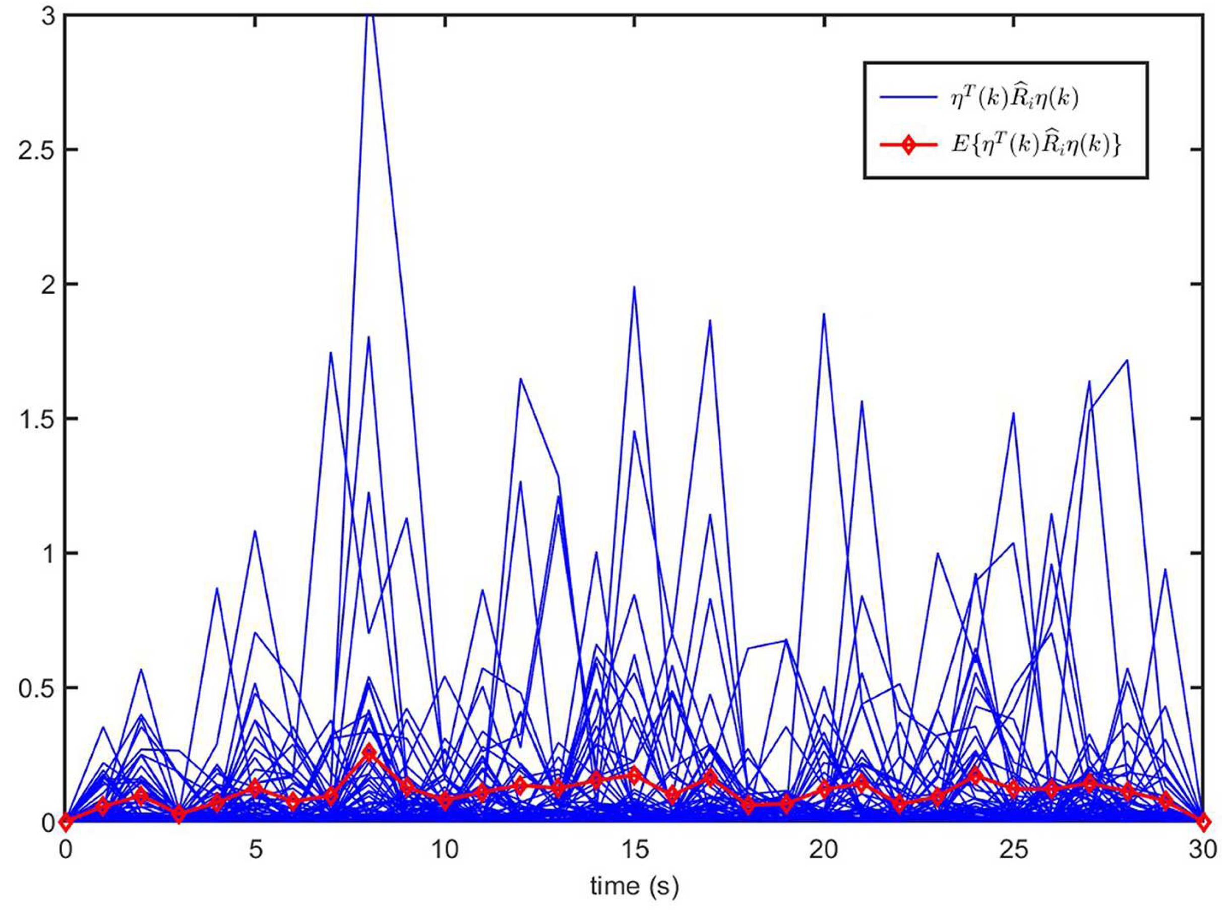
Figure 5 shows the trajectories of the system state for closed-loop system (9) and the control input of MJS (1). The trajectories of (50 curves) and of closed-loop system (9) are illustrated in Figure 6. From Figure 6, it is seen that when , , which means that the CLS (9) is SFT -bounded, that is to say, MJS (1) is SFT state feedback stabilization. Therefore, it is proven that the state feedback controller (8) designed in this paper is effective.
Next, the second example focuses on the effectiveness of the observer-based state feedback controller (32) designed in Theorem 4 for MJS (1) with partly unknown transition probabilities.
Example 2.
The parameters of MJS (1) with three modes and partly unknown TPs are given as follows:
Mode 1 ():
,
Mode 2 ():
,
Mode 3 ():
,
Then, letting , , the partly unknown TP matrix and the remaining parameters have identical values to those in Example 1. Similar to Example 1, we can obtain the feasible solution of (46) when . The relationships between and and , and between and are shown in Figure 7 and Figure 8, respectively. From Figure 7 and Figure 8, we can see that the optimal values are and with .
Then, we compare the results of Theorem 4 with Theorem 2 in [44]. The optimal values of (i.e., in [44]) and obtained from the two works are shown in Table 2.
From Table 2, it appears that the optimal values of , , and obtained in this paper are smaller than those of [44], which indicates that the results of this paper are better. In addition, ref. [44] assumed that the transition probabilities were completely known, which means that the results of [44] are special cases of this paper.
In addition, by solving LMIs (37), (39), (40), (41), and (44), we have , , and , and the gains of observer-based state feedback controller (32) are as follows:
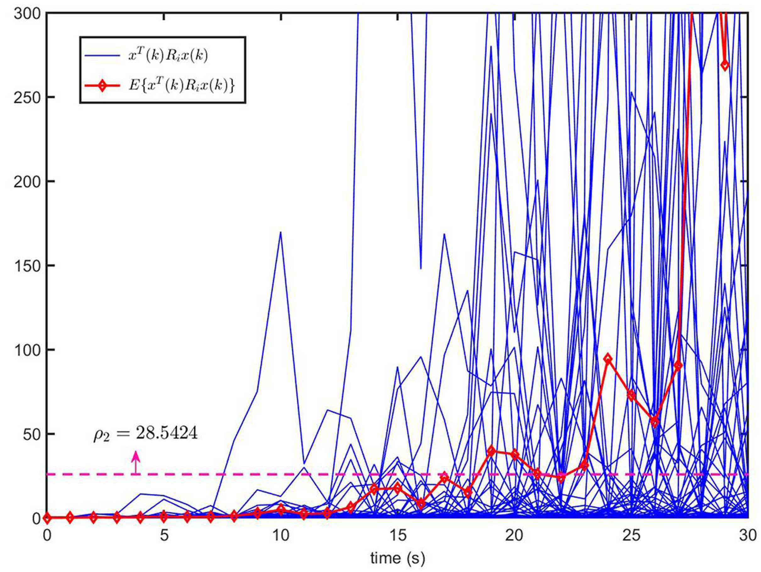
Next, we set the initial value for systems (1) and (33), respectively. The external disturbance signal is the same as in Example 1. The Markovian switching process of MJS (1) and CLS (33) is shown in Figure 9. Figure 10 shows the trajectories of (50 curves) and of open-loop system (1) , which implies that open-loop system (1) is not finite time-bound.
The trajectories of system state for CLS (33) and the curve of the control input of (32) are illustrated in Figure 11. Moreover, Figure 12 shows the trajectories of (50 curves) and of closed-loop system (33). From Figure 12, it can be observed that CLS (33) is SFT -bounded, i.e., MJS (1) is SFT observer-based state feedback stabilization. Furthermore, by comparing Figure 10 and Figure 12, it can be proven that observer-based state feedback controller (32) is effective.
6. Conclusions
Based on existing results, the design schemes of a stochastic finite-time state feedback controller and a stochastic finite-time observer-based state feedback controller for MJSs with a time delay and partly unknown TPs were studied in this paper. A state feedback controller and an observer-based state feedback controller were designed and some sufficient conditions for the CLSs to satisfy SFT boundedness were presented via LKF technology. Then, the controller gains were obtained by using the LMI method. Lastly, two examples were provided to verify the validity of the proposed design schemes. In the following work, the finite-time guaranteed cost control and event-triggered control of discrete-time MJSs will be studied on the basis of this paper.
Author Contributions
Data curation, X.G.; Writing—original draft, X.G.; Conceptualization, Y.L.; Methodology, Y.L.; Writing—review & editing, Y.L.; Supervision, X.L.; Project administration, X.L.; Funding acquisition, X.L. All authors have read and agreed to the published version of the manuscript.
Funding
This work was supported by the National Natural Science Foundation of China (No. 61972236) and the Shandong Provincial Natural Science Foundation (No. ZR2022MF233).
Institutional Review Board Statement
Not applicable.
Data Availability Statement
The data presented in this study are available on request from the corresponding author.
Conflicts of Interest
The authors declare no conflicts of interest.
References
- Liu, Z.; Karimi, H.R.; Yu, J. Passivity-based robust sliding mode synthesis for uncertain delayed stochastic systems via state observer. Automatica 2020, 111, 108596. [Google Scholar] [CrossRef]
- Li, Y.; Zhang, W.; Liu, X. H- index for discrete-time stochastic systems with Markovian jump and multiplicative noise. Automatica 2018, 90, 286–293. [Google Scholar] [CrossRef]
- Liu, X.; Zhang, W.; Li, Y. H- index for continuous-time stochastic systems with Markovian jump and multiplicative noise. Automatica 2019, 105, 167–178. [Google Scholar] [CrossRef]
- Yang, H.; Yin, S.; Kaynak, O. Neural network-based adaptive fault-tolerant control for Markovian jump systems with nonlinearity and actuator faults. IEEE Trans. Syst. Man Cybern. Syst. 2020, 51, 3687–3698. [Google Scholar] [CrossRef]
- Li, F.; Li, X.; Zhang, X.; Yang, C. Asynchronous filtering for delayed Markovian jump systems via homogeneous polynomial approach. IEEE Trans. Autom. Control. 2019, 65, 2163–2170. [Google Scholar] [CrossRef]
- Ren, J.; He, G.; Fu, J. Robust H∞ sliding mode control for nonlinear stochastic T-S fuzzy singular Markovian jump systems with time-varying delays. Inf. Sci. 2020, 535, 42–63. [Google Scholar] [CrossRef]
- Wang, Y.; Han, Y.; Gao, C. Robust H∞ sliding mode control for uncertain discrete singular T-S fuzzy Markov jump systems. Asian J. Control. 2023, 25, 524–536. [Google Scholar] [CrossRef]
- Shi, Y.; Peng, X. Fault detection filters design of polytopic uncertain discrete-time singular Markovian jump systems with time-varying delays. J. Frankl. Inst. 2020, 357, 7343–7367. [Google Scholar] [CrossRef]
- Wang, G.; Xu, L. Almost sure stability and stabilization of Markovian jump systems with stochastic switching. IEEE Trans. Autom. Control. 2021, 67, 1529–1536. [Google Scholar] [CrossRef]
- Li, X.; Zhang, W.; Lu, D. Stability and stabilization analysis of Markovian jump systems with generally bounded transition probabilities. J. Frankl. Inst. 2020, 357, 8416–8434. [Google Scholar] [CrossRef]
- Liu, X.; Zhuang, J.; Li, Y. H∞ filtering for Markovian jump linear systems with uncertain transition probabilities. Int. J. Control. Autom. Syst. 2021, 19, 2500–2510. [Google Scholar] [CrossRef]
- Pan, S.; Zhou, J.; Ye, Z. Event-triggered dynamic output feedback control for networked Markovian jump systems with partly unknown transition rates. Math. Comput. Simul. 2021, 181, 539–561. [Google Scholar] [CrossRef]
- Su, X.; Wang, C.; Chang, H.; Yang, Y.; Assawinchaichote, W. Event-triggered sliding mode control of networked control systems with Markovian jump parameters. Automatica 2021, 125, 109405. [Google Scholar] [CrossRef]
- Shen, A.; Li, L.; Li, C. H∞ filtering for discrete-time singular Markovian jump systems with generally uncertain transition rates. Circuits, Syst. Signal Process. 2021, 40, 3204–3226. [Google Scholar] [CrossRef]
- Park, C.; Kwon, N.K.; Park, I.S.; Park, P. H∞ filtering for singular Markovian jump systems with partly unknown transition rates. Automatica 2019, 109, 108528. [Google Scholar] [CrossRef]
- Xue, M.; Yan, H.; Zhang, H.; Li, Z.; Chen, S.; Chen, C. Event-triggered guaranteed cost controller design for T-S fuzzy Markovian jump systems with partly unknown transition probabilities. IEEE Trans. Fuzzy Syst. 2020, 29, 1052–1064. [Google Scholar] [CrossRef]
- Sun, H.; Zhang, Y.; Wu, A. H∞ control for discrete-time Markovian jump linear systems with partially uncertain transition probabilities. Optim. Control. Appl. Methods 2020, 41, 1796–1809. [Google Scholar] [CrossRef]
- Zhang, J.; Liu, Z.; Jiang, B. Neural network-based adaptive reliable control for nonlinear Markov jump systems against actuator attacks. Nonlinear Dyn. 2023, 111, 13985–13999. [Google Scholar] [CrossRef]
- Guo, G.; Zhang, X.; Liu, Y.; Zhao, Z.; Zhang, R.; Zhang, C. Disturbance observer-based finite-time braking control of vehicular platoons. IEEE Trans. Intell. Veh. 2023. [Google Scholar] [CrossRef]
- Hamrah, R.; Sanyal, A.K.; Viswanathan, S.P. Discrete finite-time stable attitude tracking control of unmanned vehicles on SO(3). In Proceedings of the 2020 American Control Conference (ACC), Denver, CO, USA, 1–3 July 2020; pp. 824–829. [Google Scholar] [CrossRef]
- Zhao, J.; Qiu, L.; Xie, X.; Sun, Z. Finite-time stabilization of stochastic nonlinear systems and its applications in ship maneuvering systems. IEEE Trans. Fuzzy Syst. 2023, 32, 1023–1035. [Google Scholar] [CrossRef]
- Dorato, P. Short-Time Stability in Linear Time-Varying Systems. Ph. D. Thesis, Polytechnic Institute of Brooklyn, Brooklyn, NY, USA, 1961. [Google Scholar]
- Ren, C.; He, S. Finite-time stabilization for positive Markovian jumping neural networks. Appl. Math. Comput. 2020, 365, 124631. [Google Scholar] [CrossRef]
- Zhang, Y.; Jiang, T. Finite-time boundedness and chaos-like dynamics of a class of Markovian jump linear systems. J. Frankl. Inst. 2020, 357, 2083–2098. [Google Scholar] [CrossRef]
- Chen, Q.; Tong, D.; Zhou, W. Finite-time stochastic boundedness for Markovian jumping systems via the sliding mode control. J. Frankl. Inst. 2022, 359, 4678–4698. [Google Scholar] [CrossRef]
- Zhong, S.; Zhang, W.; Feng, L. Finite-time stability and asynchronous resilient control for Itô stochastic semi-Markovian jump systems. J. Frankl. Inst. 2022, 359, 1531–1557. [Google Scholar] [CrossRef]
- Sang, H.; Wang, P.; Zhao, Y.; Nie, H.; Fu, J. Input-output finite-time stability for switched T-S fuzzy delayed systems with time-dependent Lyapunov-Krasovskii functional approach. IEEE Trans. Fuzzy Syst. 2023, 31, 3823–3837. [Google Scholar] [CrossRef]
- Kaviarasan, B.; Kwon, O.; Park, M.J.; Sakthivel, R. Input-output finite-time stabilization of T-S fuzzy systems through quantized control strategy. IEEE Trans. Fuzzy Syst. 2021, 30, 3589–3600. [Google Scholar] [CrossRef]
- Hu, X.; Wang, L.; Sheng, Y.; Hu, J. Finite-time stabilization of fuzzy spatiotemporal competitive neural networks with hybrid time-varying delays. IEEE Trans. Fuzzy Syst. 2023, 31, 3015–3024. [Google Scholar] [CrossRef]
- Li, X.; Ho, D.W.; Cao, J. Finite-time stability and settling-time estimation of nonlinear impulsive systems. Automatica 2019, 99, 361–368. [Google Scholar] [CrossRef]
- Yang, X.; Li, X. Finite-time stability of nonlinear impulsive systems with applications to neural networks. IEEE Trans. Neural Netw. Learn. Syst. 2021, 34, 243–251. [Google Scholar] [CrossRef]
- Zhang, T.; Deng, F.; Shi, P. Non-fragile finite-time stabilization for discrete mean-field stochastic systems. IEEE Trans. Autom. Control. 2023, 68, 6423–6430. [Google Scholar] [CrossRef]
- Liu, X.; Liu, Q.; Li, Y. Finite-time guaranteed cost control for uncertain mean-field stochastic systems. J. Frankl. Inst. 2020, 357, 2813–2829. [Google Scholar] [CrossRef]
- Liu, X.; Teng, Y.; Li, Y. A design proposal of finite-time H∞ controller for stochastic mean-field systems. Asian J. Control. 2024. [Google Scholar] [CrossRef]
- Sun, X.; Yang, D.; Zong, G. Annular finite-time H∞ control of switched fuzzy systems: A switching dynamic event-triggered control approach. Nonlinear Anal. Hybrid Syst. 2021, 41, 101050. [Google Scholar] [CrossRef]
- Zhu, C.; Li, X.; Cao, J. Finite-time H∞ dynamic output feedback control for nonlinear impulsive switched systems. Nonlinear Anal. Hybrid Syst. 2021, 39, 100975. [Google Scholar] [CrossRef]
- Wang, G.; Zhao, F.; Chen, X.; Qiu, J. Observer-based finite-time H∞ control of Itô -type stochastic nonlinear systems. Asian J. Control. 2023, 25, 2378–2387. [Google Scholar] [CrossRef]
- Zhang, Y.; Liu, C. Observer-based finite-time H∞ control of discrete-time Markovian jump systems. Appl. Math. Model. 2013, 37, 3748–3760. [Google Scholar] [CrossRef]
- Gao, X.; Ren, H.; Deng, F.; Zhou, Q. Observer-based finite-time H∞ control for uncertain discrete-time nonhomogeneous Markov jump systems. J. Frankl. Inst. 2019, 356, 1730–1749. [Google Scholar] [CrossRef]
- Mu, X.; Li, X.; Fang, J.; Wu, X. Reliable observer-based finite-time H∞ control for networked nonlinear semi-Markovian jump systems with actuator fault and parameter uncertainties via dynamic event-triggered scheme. Inf. Sci. 2021, 546, 573–595. [Google Scholar] [CrossRef]
- He, Q.; Xing, M.; Gao, X.; Deng, F. Robust finite-time H∞ synchronization for uncertain discrete-time systems with nonhomogeneous Markovian jump: Observer-based case. Int. J. Robust Nonlinear Control. 2020, 30, 3982–4002. [Google Scholar] [CrossRef]
- Liu, X.; Wei, X.; Li, Y. Observer-based finite-time fuzzy H∞ control for Markovian jump systems with time-delay and multiplicative noises. Int. J. Fuzzy Syst. 2023, 25, 1643–1655. [Google Scholar] [CrossRef]
- Liu, X.; Li, W.; Wang, J.; Li, Y. Robust finite-time stability for uncertain discrete-time stochastic nonlinear systems with time-varying delay. Entropy 2022, 24, 828. [Google Scholar] [CrossRef] [PubMed]
- Wei, X.; Liu, N.; Liu, X.; Li, Y. Observer-based finite-time H∞ control for discrete-time Markovian jump systems with time-delays. J. Shandong Univ. Technol. Nat. Sci. Ed. 2022, 36, 17–27. [Google Scholar] [CrossRef]

Figure 2.
The values of and with different values.

Figure 3.
The values of with different values.

Figure 4.
The trajectories of and for open-loop system (1) ().
Figure 4.
The trajectories of and for open-loop system (1) ().


Figure 7.
The optimal values of and with different values.

Figure 8.
The values of with different values.


Figure 10.
The trajectories of and for open-loop system (1) .
Figure 10.
The trajectories of and for open-loop system (1) .


Figure 12.
The trajectories of and for CLS (33).
Figure 12.
The trajectories of and for CLS (33).


Table 1.
The acronyms used in this article and their meanings.
| Acronyms | Meaning of Acronyms |
|---|---|
| MJS | Markovian jump system |
| SFT | Stochastic finite-time |
| LKF | Lyapunov–Krasovskii functional |
| CLS | Closed-loop system |
| LMI | Linear matrix inequality |
| TP | Transition probability |
Table 2.
The optimal values of , , and .
| Method | Theorem 4 in This Paper | Theorem 2 in Reference [44] |
|---|---|---|
| 9.6193 | 105.9526 | |
| 28.5424 | 150.4146 | |
| 121.0731 | 11,376.368 |
Disclaimer/Publisher’s Note: The statements, opinions and data contained in all publications are solely those of the individual author(s) and contributor(s) and not of MDPI and/or the editor(s). MDPI and/or the editor(s) disclaim responsibility for any injury to people or property resulting from any ideas, methods, instructions or products referred to in the content. |
© 2024 by the authors. Licensee MDPI, Basel, Switzerland. This article is an open access article distributed under the terms and conditions of the Creative Commons Attribution (CC BY) license (https://creativecommons.org/licenses/by/4.0/).
Share and Cite
MDPI and ACS Style
Guo, X.; Li, Y.; Liu, X. Finite-Time H∞ Controllers Design for Stochastic Time-Delay Markovian Jump Systems with Partly Unknown Transition Probabilities. Entropy 2024, 26, 292. https://0-doi-org.brum.beds.ac.uk/10.3390/e26040292
AMA Style
Guo X, Li Y, Liu X. Finite-Time H∞ Controllers Design for Stochastic Time-Delay Markovian Jump Systems with Partly Unknown Transition Probabilities. Entropy. 2024; 26(4):292. https://0-doi-org.brum.beds.ac.uk/10.3390/e26040292
Chicago/Turabian StyleGuo, Xinye, Yan Li, and Xikui Liu. 2024. "Finite-Time H∞ Controllers Design for Stochastic Time-Delay Markovian Jump Systems with Partly Unknown Transition Probabilities" Entropy 26, no. 4: 292. https://0-doi-org.brum.beds.ac.uk/10.3390/e26040292
Note that from the first issue of 2016, this journal uses article numbers instead of page numbers. See further details here.