
Efficient Implementation of Discrete-Time Quantum Walks on Quantum Computers


1
Center for Nonlinear and Complex Systems, Dipartimento di Scienza e Alta Tecnologia, Università degli Studi dell’Insubria, Via Valleggio 11, 22100 Como, Italy
2
Istituto Nazionale di Fisica Nucleare, Sezione di Milano, Via Celoria 16, 20133 Milano, Italy
3
Istituto di Fotonica e Nanotecnologie, Consiglio Nazionale delle Ricerche, Via Valleggio 11, 22100 Como, Italy
4
National Enterprise for nanoScience and nanoTechnology, Istituto Nanoscienze-CNR, Piazza San Silvestro 12, 56127 Pisa, Italy
*
Author to whom correspondence should be addressed.
Entropy 2024, 26(4), 313; https://0-doi-org.brum.beds.ac.uk/10.3390/e26040313
Submission received: 13 February 2024
/
Revised: 27 March 2024
/
Accepted: 28 March 2024
/
Published: 2 April 2024
(This article belongs to the Special Issue Quantum Walks for Quantum Technologies)
Abstract
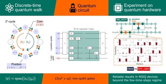
:Quantum walks have proven to be a universal model for quantum computation and to provide speed-up in certain quantum algorithms. The discrete-time quantum walk (DTQW) model, among others, is one of the most suitable candidates for circuit implementation due to its discrete nature. Current implementations, however, are usually characterized by quantum circuits of large size and depth, which leads to a higher computational cost and severely limits the number of time steps that can be reliably implemented on current quantum computers. In this work, we propose an efficient and scalable quantum circuit implementing the DTQW on the -cycle based on the diagonalization of the conditional shift operator. For t time steps of the DTQW, the proposed circuit requires only two-qubit gates compared to the of the current most efficient implementation based on quantum Fourier transforms. We test the proposed circuit on an IBM quantum device for a Hadamard DTQW on the 4-cycle and 8-cycle characterized by periodic dynamics and by recurrent generation of maximally entangled single-particle states. Experimental results are meaningful well beyond the regime of few time steps, paving the way for reliable implementation and use on quantum computers.
1. Introduction
Quantum walks were formally introduced in the 1990s as the quantum analogue of classical random walks [1,2], but the seminal concept dates back to Feynman’s checkerboard (see Problem 2–6 in [3]), which connects the spin with the zig-zag propagation of a particle spreading at the speed of light across a (1 + 1)-dimensional spacetime lattice. The great potential of exploiting the peculiar features of quantum walks—quantum superposition of multiple paths, ballistic spread (faster than the diffusive spread of a classical random walker), and entanglement—for algorithmic purposes [4,5,6] has been immediately clear since their introduction. Nowadays, quantum walks have proven to be a universal model for quantum computation [7,8,9,10,11], and examples of their use include algorithms for quantum search [12,13,14,15]; the solving of hard K-SAT instances [16]; graph isomorphism problems [17,18,19]; algorithms in complex networks [20,21] such as link prediction [22,23] and community detection [24,25]; and quantum simulation [26,27,28,29,30]. Furthermore, quantum communication protocols based on quantum walks have been put forward [31,32,33,34,35,36,37,38,39]. For comprehensive reviews on quantum walks and their applications, we refer the reader to [40,41,42] and to [43,44,45] for the their physical implementations.
There are two main models of the quantum walk: the discrete-time quantum walk (DTQW) [1] and the continuous-time quantum walk (CTQW) [2]. The CTQW is defined on the position Hilbert space of the quantum walker, and the evolution is driven by the Hamiltonian H of the system, . The DTQW is defined on a Hilbert space comprising an additional coin space, and the evolution is driven by a position shift operator, S, controlled by a quantum coin operator, C, acting at discrete time steps. The single time-step operator is defined as , where is the identity in position space, from which with . As pointed out in [46], implementing the evolution operator of a DTQW is simplified by the fact that (i) the time is discrete, (ii) the evolution is repetitive, , and (iii) U acts locally on the coin–vertex states encoding the graph (applying U to the coin–vertex states associated with a given vertex will propagate the corresponding amplitudes only to adjacent vertices).
DTQWs already have efficient physical implementations in platforms that natively support the conditional walk operations, e.g., photonic systems [44,45]. However, devising efficient implementations on digitized quantum computers is desirable and necessary in order to make DTQWs available to develop quantum algorithms for general purpose quantum computers and, in general, quantum protocols to be implemented in circuit models. A first circuit implementation of a DTQW on the cycle was realized on a multiqubit nuclear magnetic resonance system [47], and thereafter, proposals for efficient implementation on certain graphs [48,49,50,51], for position-dependent coin operators [52], and for staggered quantum walks (a coinless discrete-time model of quantum walk) [53] have been devised.
In this work, we propose an efficient and scalable quantum circuit implementing the DTQW on the -cycle, a finite discrete line with vertices and periodic boundary conditions. Although this is the simplest DTQW one may think of, implementing it on quantum computers already highlights the limitations of actual quantum devices [54,55,56,57]. In this model, the position state of the quantum walker is encoded in an n-qubit state. To the best of our knowledge, the most efficient state-of-the-art implementation of a DTQW [58] overall requires two-qubit gates for t time steps, because it involves one quantum Fourier transform (QFT) and one inverse QFT (IQFT) at each time step. In quantum computers, two-qubit gates are the noisiest and take the longest time to execute, so any efficient quantum circuit should aim at significantly reducing their number. Our quantum circuit accomplishes this task through a wise use of the unitary property of the QFT: independent of t, our circuit involves only one QFT (at the beginning) and one IQFT (at the end), and thus, it overall requires two-qubit gates. Accordingly, the advantage becomes larger and larger for long times, passing, for , from in [58] to in the present scheme. For illustrative purposes, we implemented the proposed quantum circuit on actual quantum hardware—ibm_cairo v.1.3.5, a 27-qubit high-fidelity quantum computer—considering a Hadamard DTQW on the 4- and 8-cycles. Results indicate that our circuit outperforms current efficient circuits also in the regime of few time steps and provides experimental evidence of the recurrent generation of maximally entangled single-particle states in the 4-cycle [59].
This paper is organized as follows. Section 2 reviews the DTQW model on the N-cycle. Section 3 introduces the efficient quantum circuit we designed for the DTQW on the -cycle and compares it with other existing schemes. Section 4 presents and discusses the results from testing the proposed circuit on quantum hardware. Finally, Section 5 is devoted to conclusions and perspectives. Selected technical details are deferred to the Appendices.
2. The Model: DTQW on the N-Cycle
An N-cycle, or circle, is a 1D lattice having N vertices and periodic boundary conditions. To each vertex, labeled by , we associate a quantum state, , which represents the walker localized at such a vertex. In a DTQW, the quantum walker has an external degree of freedom, the position, and an internal one, the coin. Associated with each degree of freedom is a Hilbert space: an N-dimensional position Hilbert space and a two-dimensional coin Hilbert space . We use the label “p” to refer to the walker’s position degree of freedom and “c” to the coin degree of freedom. Depending on the coin state, the walker can move counterclockwise () or clockwise () on the cycle (Figure 1). The full Hilbert space is
This is the natural basis for a DTQW, and in the following, we will refer to it as the computational basis. The coin basis states are and , with ⊺ denoting the transpose without complex conjugation; the position basis states are , with the only nonzero element in position j. Accordingly, a generic coin–position basis state is represented by the column vector of length , whose first N entries are related to and the last N to . The only nonzero entry is the -th one.
Figure 1.
Schematic representation of a DTQW on the N-cycle. (a) The coin state (internal degree of freedom) is responsible for making the walker move in the cycle clockwise if and counterclockwise if . (b) States and operators of a DTQW. The vertices of the cycle (light violet)—walker’s position states—are labeled by with , and each vertex comprises two subvertices—coin states—labeled by (orange) and (green). Each step of the walk, Equation (2), involves the action of a local coin operator responsible for mixing the coin states of each vertex (we assume ), followed by the action of the conditional-shift operators (decrement) and (increment) responsible for shifting the position states, see Equation (3) [43].

The evolution is ruled by the unitary single time-step operator
where is the identity in position space and C the coin operator acting on the coin state. Coin and conditional shift operators must be unitary for U to be unitary. The conditional shift operator S acts on the full Hilbert space and makes the walker move according to the coin state: , where operations in position space are performed modulo N. Such an operator can be written as
where . The operators (decrement) and (increment) are responsible for making the walker move one step counterclockwise and clockwise, respectively, (see Figure 1 and Figure 2b,c). In the computational basis, the conditional shift operator (3) has the matrix representation
where is the null matrix and
The quantum walker is usually assumed to be initially localized at the vertex , while the coin is in a generic superposition state,
with and . After time steps, the quantum walker will be in the state
where the amplitudes —with —associated with the states satisfy the normalization condition at any t, . The probability to find the walker at position k at time t, irrespective of the coin state, is .
3. Quantum Circuit Implementing the DTQW on the -Cycle
A quantum circuit implementing the DTQW on the N-cycle with requires qubits: n to encode the walker’s position state and an additional 1 to encode the coin state. Both states are encoded in base 2. Denoting by the binary representation of the integer j with n digits, in the little-endian ordering convention (the most significant bit is placed on the left), we write
where with , such that . Accordingly, we write the quantum state of the quantum walker as the -qubit state
which represents the state where the coin is in the state and the walker is in the position state .
3.1. Quantum Circuit Design
The efficiency of a quantum circuit implementing a DTQW relies on the efficient implementation of the single time-step operator (2), so, ultimately, on that of the conditional shift operator (3). As shown in Equation (4), the latter involves the circulant matrices and introduced in Equation (5), and circulant matrices are known to be diagonalized by the quantum Fourier transform (QFT) matrix (see Appendix A). The QFT of the computational basis is defined as
where and , with matrix representation . The inverse QFT (IQFT) is represented by . The QFT is a unitary transformation, . Accordingly, we can write
where
with
We stress that (order matters) and that we can write the second equality of Equation (12) because we are assuming . Given Equation (11), the conditional shift matrix S (4) and its diagonal form are related via
where the identity in coin space is required since the (I)QFT acts on position space only.
The DTQW of t steps is generated by repeatedly applying the operator U t times, Equation (7). Recalling that the QFT is unitary, it acts only on position space, and given that and that , we can write
with in Equation (14). Equation (15) provides a first sketch of the circuit we are going to implement. First, we perform a QFT on the position register, . Then, we repeat t times the single time-step evolution in the extended Fourier space (extended to include coin space), . In the end, we perform an IQFT on the position register, . Even at this stage, an advantage of our scheme is evident: overall, it requires only one QFT and one IQFT, unlike the QFT scheme in Figure 3, which requires both the transformations at each time step [58].
Now, we focus on to further improve the above scheme. The second equality in Equation (14) clearly shows the action of : if the coin is in the state (), then the operator () acts on the position state. It is evident that, in the present form, each step of the DTQW requires controlled- gates. To reduce the number of controlled operations, we point out that performing on the k-th position qubit if the coin is in the state and (opposite phase) if in is equivalent to performing regardless of the coin state, followed by a controlled- if the coin is in to compensate the previously assigned phase and obtain the correct one. Formally, we can rewrite the diagonal conditional shift operator (14) as
where
since and (one-qubit identity gate), see Equation (13).
As a final step in optimizing our quantum circuit, we want to make the SWAP operations, usually required in a proper (I)QFT to obtain the correct states, unnecessary. Therefore, following the argument in [58], it is useful to introduce the SWAP operation on the n-qubit register, which we denote by . The SWAP takes qubit k to qubit and vice versa,
This operation is unitary, , and involutory, . A proper (I)QFT on n qubits requires a SWAP on the n-qubit register at the end (beginning) of the circuit, i.e.,
where denotes the (I)QFT without the SWAP. Similarly, we introduce
see Equation (12). Using Equations (19)–(20) and recalling that acts only on the position register (not on the coin), we observe that
according to which we can rewrite Equation (15) as
In conclusion, the quantum circuit implementing t steps of a DTQW, excluding the initial state preparation, is shown in Figure 4 and does not need the SWAP in the (I)QFT. Size and depth of a quantum circuit implementing a DTQW can be further reduced by choosing a proper encoding of the position space and designing initial-state-dependent circuits [60]. We point out that the design of our quantum circuit is independent of the initial state, but it can be further optimized for an initially localized walker, the usual initial condition, by replacing the initial QFT with a layer of Hadamard gates (Appendix B).
3.2. Comparison with Other Existing Schemes
In this section, we estimate the size of the proposed quantum circuit (Figure 4) in terms of depth and number of one- and two-qubit gates, and , respectively, and compare it with those of other existing schemes, following the preliminary analysis provided in [58]. We compare our scheme with the following ones: (i) The ID scheme [48], which is based on the increment and decrement gates (Figure 2) that require generalized CNOT gates. The latter can be implemented in different ways, so, as an example, we consider their implementation (i.a) via linear-depth quantum circuit [61] or (i.b) via ancilla qubits [62]. In passing, we also mention a possible implementation via rotations [56]. In the following analysis, we consider the ID scheme implemented as in Figure 2d, with the increment gate only. (ii) The QFT scheme [58], which is based on the increment gate diagonalized by the QFT (Figure 3).
This discussion is neither supposed to be exhaustive, e.g., there are several ways to implement the generalized CNOT gates in the ID scheme, nor supposed to provide optimal and universal metrics, as the latter are ultimately quantum-device-dependent, e.g., it suffices to think of the process of transpilation, which rewrites and/or optimizes a given circuit according to the topology of the quantum device considered. Still, our estimate is useful to show how our scheme scales better than others when including the number of implemented time steps in the analysis, in particular if compared to the QFT scheme (Figure 3), which is, to the best of our knowledge, the most efficient state-of-the-art implementation of DTQW on -cycles. Results of the circuit size in the different schemes are summarized in Table 1 and shown in Figure 5. Details of the computation are deferred to Appendix C.
Considering both the number n of position qubits and the number t of time steps, the ID scheme is the most resource-demanding among those examined: (i.a) If generalized CNOT gates are implemented via linear-depth quantum circuits, then the circuit’s depth increases as and the results quickly degrade due to the large number of two-qubit gates, . (i.b) If generalized CNOT gates are implemented via ancilla qubits, then the circuit’s depth is of the same order, , but the number of two-qubit gates is reduced by an order, , at the cost of requiring extra qubits, . Both the ID approaches require . (ii) A remarkable improvement is obtained by the QFT scheme, which, with no need of ancilla qubits, has and , at the cost of increasing the number of one-qubit gates, . Our scheme refines such metrics by making the cost of the (I)QFT independent of the number of time steps: in the long time limit, , we have , to which is added a fixed, t-independent but n-dependent, cost , , and . To ease the comparison among the schemes, the metrics of Table 1 are shown in Figure 5, making it clear that our scheme outperforms the others in the number of two-qubit gates, which take the longest time to execute and are the noisiest in quantum computers. Furthermore, we observe that the circuit depth is mainly determined by the number of two-qubit gates.
In conclusion, both the QFT scheme and ours outperform the ID scheme at any time. Although these metrics are comparable in the few-time-steps regime, our scheme outperforms the QFT scheme when a large number of time steps is implemented.
4. Results and Discussion
We test the DTQW circuit introduced in Section 3.1 (see Figure 4) on the IBM quantum computer ibm_cairo v.1.3.5, a 27-qubit Falcon r5.11 processor whose qubit connectivity map is shown in Figure 6a. The IBM Quantum system ibm_cairo is remotely accessed via the IBM cloud computing services [63] and experiments are run within the Qiskit framework [64]. In the following, we introduce the DTQW considered for the test and the quantities of interest, then we point out some solutions to improve the circuit, and finally we present and discuss the results.
4.1. Hadamard DTQW
A common choice for the coin operator is the Hadamard coin
As for the initial state, we assume the walker to be initially localized in and the coin to be in a given superposition
The Hadamard DTQW for this initial state has the following properties: (i) The dynamics is periodic of period () on the 4-cycle (8-cycle) [65]. (ii) Maximally entangled single-particle states—entanglement between position and coin—are generated after one step of the walk and then recurrently with period () on the 4-cycle (8-cycle) [59]. These properties are therefore suitable for thoroughly testing the quality of the designed quantum circuit, i.e., to assess to what extent the actual implementation can reproduce these ideal features. We point out that for a Hadamard DTQW on the 4- and 8-cycles, any initial state (6) with will generate a dynamics with the two above-mentioned features for any value of [59]. We arbitrarily set to initialize the coin in a nontrivial superposition of states, see Equation (23). For later convenience, we anticipate that the periodic dynamics of the DTQW on the 4- and 8-cycles will sustain the periodic occurrence of localized states when the initial state is localized in position space. However, dynamics and occurrence of localized states can have different periods. In the 4-cycle, the initial state localized in is perfectly transferred to after four time steps; hence, localized states occur with period , in contrast with the period of the dynamics. Instead, in the 8-cycle, localized states occur only as a result of the periodic dynamics () [59]. Implementing the cycle with and vertices requires and position qubits, respectively.
4.2. Figures of Merit
Probability distribution: In most DTQW problems, we are interested in the probability distribution of the walker’s position. Our purpose is to compare the ideal probability distribution with the experimental ones, the latter obtained in a noisy simulation and in an actual implementation on the quantum hardware ibm_cairo. To compare two discrete probability distributions, and , we adopt the Hellinger fidelity , where the Hellinger distance [66] between P and Q is defined by
The Hellinger distance is symmetric, , and bounded , where the value means that the two distributions are equal (fidelity ).
Entanglement: Usually, in a DTQW, entanglement between walker and coin occurs. This can be understood as hybrid entanglement, also referred to as single-particle entanglement because it is established between different degrees of freedom of the same quantum system, here position and coin, which is an internal degree of freedom, e.g., spin [67]. Bipartite entanglement can be probed by means of entanglement entropies. In this case, we probe the second-order Rényi entanglement entropy [68] of the reduced density matrix for the two parts (coin and position) via randomized measurements [69]. Estimating this quantity requires significantly fewer measurements than performing quantum state tomography: for an n-qubit state, with (the coefficient a depends on the nature of the considered state, see Supplementary Materials for [69]) compared to [70]. In this regard, the advantage of this approach becomes remarkable when a large number of qubits is involved—as expected to be in future applications—due to the current costliness of tomography. The second-order Rényi entropy for a part A of the total bipartite system described by is defined as
where is the reduced density matrix for part A. If the second-order Rényi entropy of the part is greater than that of the total system, , then bipartite entanglement exists between the two parts (for separable states and [68]). If, in addition, the overall state is pure, then the second-order Rényi entropy is directly a measure of bipartite entanglement and (the reduced density matrices of a pure bipartite state have the same nonzero eigenvalues, due to the Schmidt decomposition). The second-order Rényi entropy is maximum for the maximally mixed state, , with the dimension of . Furthermore, is indicative of the overall purity of the system, because it is null for pure quantum states.
4.3. Circuit Optimization
Each time step of the DTQW requires the coin qubit to interact with each position qubit (see controlled- gates in Figure 4). The quantum hardware may have limited connectivity, therefore SWAP operations are needed to make two qubits interact whenever the latter are not physically adjacent. A wise circuital implementation must account for the connectivity of the quantum hardware considered. We can limit the number of SWAPs by making the coin qubit as “shared” as possible, compatibly with the typical sparse connectivity of superconducting quantum computers. The qubit topology of ibm_cairo (Figure 6a) makes it possible to implement the circuit for a DTQW on the 4- and 8-cycles without SWAPs by mapping coin and position qubits as in Figure 6b and c, respectively. Given the optimal mapping that is compatible with the given qubit connectivity, we consider the set of qubits having the lowest error rates averaged over different calibrations. In addition, the initial state (23) being localized in position space, we replace the initial QFT with a layer of Hadamard gates (Appendix B).
4.4. Analysis of the DTQW on the 4- and 8-Cycles
Probability distribution (4-cycle): Performing a noisy simulation of the quantum circuit is the preliminary step before the actual implementation on the quantum hardware. Figure 7a shows the Hellinger fidelities of the walker’s position distribution on the 4-cycle. The Hellinger fidelity for the noisy simulation of our circuit is above for all the 19 time steps implemented, while the results for the noisy simulation of the circuit in the QFT scheme [58] degrade below the after a few steps. The previous analysis on the circuit size proved the advantage of our circuit in the long time limit, but these results suggest that our circuit outperforms the QFT scheme circuit already in the few-time-steps regime. For the actual implementation on ibm_cairo, we consider two levels of optimization in the transpilation: (i) optimization_level=1 (default value), which transpiles the circuit into the native gates of the hardware and performs a light optimization (blue dashed line, curve “IBM Cairo”), and (ii) optimization_level=3, which performs the heaviest optimization (red solid line, curve “IBM Cairo Opt.”).
The Hellinger fidelity for the default implementation of our circuit (optimization_level=1) shows a moderate discrepancy with respect to the noisy simulation but closely follows the trend of the latter. The heavily optimized implementation of our circuit (optimization_level=3) provides better results and also partially mitigates the local minima of the noisy simulation. However, we point out that the circuit transpiled with the highest optimization level turns out to have a depth which is basically independent of the number of time steps implemented (see Appendix D). This explains the long-lasting optimality of the results, up to (last time step implemented). However, this optimal transpiled circuit is obtained only for position qubits (4-cycle); for (8-cycle), we obtain a circuit whose depth increases with the number of time steps. The Hellinger fidelity at is lower than 1 because we still implement the whole circuit with , i.e., we do not just implement the initial state. Furthermore, the Hellinger fidelity is characterized by periodic local minima, with period 4 being half of the period of the dynamics. These minima occur when the walker is ideally localized in position, a probability distribution so peaked (delta) that it can hardly be obtained as the result of an actual, noisy implementation (see Figure 7b). The frame in Figure 7b shows that the walker has returned to the initial position, as expected for the periodic dynamics.
Probability distribution (8-cycle): We obtain qualitatively analogous results also for the DTQW on the 8-cycle (Figure 8). However, as anticipated in the previous paragraph, in this case, the optimization in the transpilation is not as effective as for the 4-cycle. The Hellinger fidelities with optimization_level=1 and 3 are thus consistent with each other. Unlike the DTQW on the 4-cycle, given an initial localized state, localized states at later times occur only as a result of the periodic dynamics (), hence the minimum of the Hellinger fidelity at .
Entanglement (4-cycle): Probing the second-order Rényi entanglement entropy via randomized measurements [69] for many time steps of the DTQW and for increasing size of the cycle is computationally demanding. Therefore, to discuss the recurrent generation of maximally entangled single-particle states, we focus only on the DTQW on the 4-cycle (Figure 9). First, we review the ideal scenario. Given an initial pure state and a unitary evolution, the second-order Rényi entropy of coin state, , and position state, , are equal, , and that of the total system, , is null (pure state) at any time t. Furthermore, we have , the two-dimensional coin being the part with the lowest dimension. The initial state in Equation (23) is pure and separable (no entanglement), as is the state at
which is perfectly transferred in position space from to . The dynamics has period , thus at with and , denoting the absence of entanglement when periodic separable states occur. In addition, maximally entangled single-particle states are generated at and
and are later supported by the periodic dynamics, thus at with and . For the remaining time steps, and , partially entangled states are expected (see Supplementary Materials of [59]).
Experimentally (Figure 9), the second-order Rényi entropy of the total bipartite system is nonzero even at and increases with time, denoting a further degradation of the purity of the state. Since the latter is not pure, in general we expect (the upper bound refers to the maximally mixed three-qubit state), and different maximum values, and (4-cycle). Whenever separable states are expected (), we observe local minima of , but either part has , thus denoting the presence of residual entanglement. Whenever maximally entangled single-particle states are expected (), we observe local maxima of , with , both of which are greater than up to . For the remaining time steps, we observe that at least either part has , consistent with the expected presence of partial entanglement.
To summarize, the actual multiqubit state implemented on the quantum hardware and then processed by the quantum circuit is generally mixed and characterized by residual entanglement, but the local minima and maxima of and are perfectly consistent with the expected periodic separable and maximally entangled single-particle states, respectively, up to . Results suggest that the observed local maxima will preserve the expected periodicity for further steps , but eventually due to the degradation of the purity of the total state. Entanglement is a distinct quantum signature and, in this example, we have clear evidence of generation up to . This does not necessarily imply that quantum features, including entanglement, in the realization of the DTQW are lost thereafter. Indeed, for the remaining time steps investigated, , we still observe —presence of entanglement—whenever states with partial or maximum entanglement are expected. Therefore, quantum features are present up to the last time step considered, .
5. Conclusions
We proposed an efficient quantum circuit for the DTQW on the -cycle. Our scheme, using only one QFT and one IQFT, significantly improves the most efficient state-of-the-art implementation [58] (referred to as QFT scheme in the following) which uses one QFT and one IQFT at each time step. As a result, our circuit requires only two-qubit gates, compared to the of the QFT scheme. The improvement in this gate count is even more significant for long times, passing, for , from in the QFT scheme to in ours. Therefore, since two-qubit gates take the longest time to execute and are the noisiest, our quantum circuit is computationally less demanding and paves the way for reliable implementation in noisy–intermediate-scale quantum devices [71,72,73].
In this regard, we tested the proposed quantum circuit on actual quantum hardware, ibm_cairo, considering a Hadamard DTQW on the 4- and 8-cycles. Both are characterized by periodic dynamics [65] and by recurrent generation of maximally entangled single-particle states [59]. We claim two main results. First, even in the short time regime, the present quantum circuit outperforms the current state-of-the-art DTQW circuits, whose results are degraded after only a few steps [56,58]. Despite the moderate discrepancy, our implementation on actual quantum hardware provides results that closely follow those from the noisy simulation. In particular, the Hellinger fidelity between the ideal probability distribution of the walker’s position and the experimental one is above for all the time steps we implemented in the 4-cycle and above up to time steps in the 8-cycle. Second, for the DTQW on the 4-cycle, we provide experimental evidence of the recurrent generation of nearly maximally entangled single-particle states up to time steps. The expected maximum entanglement is not achieved because the ideally pure state of the bipartite system is actually implemented on the quantum hardware as a mixed multiqubit state, and its purity degrades over time.
The implementation of our circuit on actual quantum computers may benefit from the following. The circuit strongly relies on controlled -gates (phase-shift gate), and the latter can be efficiently implemented using a single ancillary qubit [74]. Moreover, as the position space increases, the sparse connectivity of a superconducting quantum computer results in large experimental overheads of SWAP gates, which becomes unavoidable, e.g., to make the coin qubit interact with each position qubit. In this regard, a virtual two-qubit gate can be employed to suppress errors due to the additional SWAP gates [75]. Alternatively, an implementation on a quantum hardware architecture with full connectivity [76,77,78] may be more advantageous.
Possible applications of our scheme include the circuital implementation of direct communication protocols [35,36] and quantum key distribution protocols [38] based on DTQW on the cycle. We point out that the proposed circuit does not impose constraints on the coin operator (one-qubit gate), which in principle can be changed at each time step. Parrondo’s paradox arises when losing strategies are combined to obtain a winning one and it cuts across various research areas. This counterintuitive phenomenon can be observed in DTQW on the line or cycle when two or more coin operators are applied in a deterministic sequence [79,80]. Therefore, we expect that our quantum circuit may also be of interest to quantum game theory [81].
Circuit implementations of DTQW on a cycle of arbitrary N have been addressed in [51,58], while our proposal is limited to DTQW on the N-cycle with . We point out, however, that any circulant matrix is diagonalized by the QFT, and this has been already exploited to efficiently implement CTQWs on circulant graphs [82]. Similarly, our implementation for DTQWs can be generalized to circulant graphs—graphs whose adjacency matrix is circulant—which, being d-regular (each vertex has degree d), will require a d-dimensional coin [83,84]. A generalization of our approach to more complex structures is therefore desirable and potentially of larger interest, e.g., for algorithmic purposes.
Author Contributions
L.R. conceived the idea and supervised the work, with inputs from G.C., M.B., and G.B., and drafted the manuscript. G.C. performed quantum simulations by coding actual IBM quantum processors. All authors discussed the results and contributed to revision of the manuscript. All authors have read and agreed to the published version of the manuscript.
Funding
L.R., G.C., and G.B. acknowledge the financial support of the INFN through the project ‘QUANTUM’. M.B. acknowledges financial support from NQSTI within PNRR MUR project PE0000023-NQSTI.
Institutional Review Board Statement
Not applicable.
Informed Consent Statement
Not applicable.
Data Availability Statement
The dataset generated and analyzed in the current study is available from the corresponding author upon reasonable request.
Acknowledgments
We acknowledge the use of IBM Quantum services and the access to them granted by INFN for this work. The views expressed are those of the authors and do not reflect the official policy or position of IBM or the IBM Quantum team.
Conflicts of Interest
The authors declare no conflicts of interest. The funders had no role in the design of the study; in the collection, analyses, or interpretation of data; in the writing of the manuscript; or in the decision to publish the results.
Abbreviations
The following abbreviations are used in this manuscript:
| CTQW | Continuous-time quantum walk |
| DTQW | Discrete-time quantum walk |
| (I)QFT | (Inverse) quantum Fourier transform |
Appendix A. Eigenvalues and Eigenvectors of Circulant Matrices
Let C be an circulant matrix [85]
where each row is a cyclic shift of the row above it. The structure can also be characterized by noting that
The eigenvalues and eigenvectors (column vector) of C, solutions of , are
with and the symbol ⊺ denoting the transpose without complex conjugation. Letting , we have
where U is the unitary matrix
whose elements read , with . Since they have the same definition, in and U we recognize, respectively, the quantum Fourier transform, , and its inverse, . Therefore, in our framework, diagonalizing a circulant matrix C satisfies
As a case study, we consider the eigenproblem for the circulant matrices and in Equation (5). According to the notation introduced above for circulant matrices (A1) and their eigenvalues (A3), the matrix is defined by the elements , its eigenvalues are , and so its diagonal form is the matrix with defined in Equation (12). The matrix is defined by the elements , its eigenvalues are , since , and so its diagonal form is the matrix .
Appendix B. Optimization of the Circuit for an Initially Localized Walker
The initial state of a DTQW is typically assumed to be in the factorized form
The coin is in a generic state , which can be realized by a proper unitary, , starting from the default qubit state initialized to . Without loss of generality, the walker is localized in the 0-th vertex. Indeed, any DTQW with an initially localized walker can be mapped onto a DTQW with a walker initialized in because of the equivalence, under cyclic permutation, of all the vertices in a cycle. According to Equation (15), the first matrix acting on the initial state performs a QFT on the walker’s position register. If the walker was in a generic position state, then the whole QFT circuit would be required (see Figure 4). However, given the initial state (A8) and Equation (10), we observe that
where is the Hadamard gate acting on the m-th qubit and . Therefore, assuming the initial state (A8), we simply need a layer of Hadamard gates. This is much more convenient than using the whole QFT circuit, because Hadamard gates are one-qubit gates and can thus be executed in parallel. As a final remark, we point out that the above argument is unaffected from having used (I)QFT without SWAP gates in the circuit in Figure 4, since with defined in Equation (18).
Appendix C. Analysis of the Size of DTQW Quantum Circuits in Different Schemes
In this appendix, we provide details on the computation of the metrics—depth , number of one- and two-qubit gates, and , respectively—of the quantum circuits implementing a DTQW on the -cycle reported in Table 1. A few remarks are as follows:
- (i)
- The ID scheme here considered and the QFT scheme are based on the same circuit design (Figure 2d), in which the coin gate (one-qubit gate) cannot be executed in parallel to the CNOT gates, because it acts on their control qubit. Hence, the coin gate has unit depth and prevents the simplification of CNOT gates when iteratively concatenating the single time-step quantum circuit to obtain the successive steps. Therefore, in Appendix C.1 and Appendix C.2, the analysis focuses on a single time step, because the size of a circuit implementing t time steps is t times the size of that implementing a single time step.
- (ii)
- Controlled gates having different target qubits but the same control qubit (here, it is the coin) are executed in sequence (not in parallel) in actual quantum computers. This affects the depth of circuits and regards the CNOT gates in the ID and QFT schemes (Appendix C.1 and Appendix C.2, respectively) and the controlled- gates in our scheme (Appendix C.3).
- (iii)
- The (I)QFT on an n-qubit register (no SWAP) requires n one-qubit gates (Hadamard) and two-qubit gates (controlled-) and has depth [86]. This regards the analysis of the QFT scheme (Appendix C.2) and our scheme (Appendix C.3).
Appendix C.1. ID Scheme
We refer to the quantum circuit proposed in [48] as the ID scheme (Figure 2a–c), being based on increment and decrement gates. In particular, we assume the circuit to be designed as in Figure 2d, because it was proved to be equivalent but more efficient (lower size and depth) than the standard ID scheme in Figure 2a–c [58]. This design requires only the increment gate (not controlled by the coin qubit) and a sequence of CNOT gates (two-qubit gates, depth ; see remark (ii)). In this context, different realizations of the ID scheme stem from different implementations of the generalized CNOT gates in the increment gate. In the following, we will refer to the generalized CNOT on qubits as the k-Toffoli gate, i.e., a gate where one qubit is flipped conditional on the other (control) qubits being set to 1. A 3-Toffoli gate () denotes the standard Toffoli gate. The increment gate on the n-qubit register (walker’s position, see Figure 2b) requires k-Toffoli gates—with , i.e., ; one Toffoli gate (, i.e., ); one CNOT (, two-qubit gate); and one NOT (, one-qubit gate); see Figure 2b.
Implementation via linear-depth quantum circuit: A k-Toffoli gate, with , can be implemented using a linear-depth quantum circuit having , , and [61]. The increment gate (Figure 2b) has , , and . Therefore, the overall quantum circuit implementing the single time step of the DTQW (Figure 2d) has
Implementation via ancilla qubits: A k-Toffoli gate, with , can be implemented using ancilla qubits and Toffoli gates [62]. Accordingly, size and depth of this k-Toffoli gate are proportional to those of the Toffoli gate (), which can be realized, e.g., with a linear-depth quantum circuit having , , and (see previous paragraph) [61]. The increment gate (Figure 2b), in addition to one CNOT and one NOT, requires overall Toffoli gates (one standard Toffoli gate plus the decomposition of k-Toffoli gates with ), so it has , , and . Therefore, the overall quantum circuit implementing the single time step of the DTQW (Figure 2d) has
The number of ancilla qubits is independent of the number of time steps t and is determined by the k-Toffoli gate having the largest number of controls, as the ancilla qubits can be reused among the k-Toffoli gates of the increment gate [58].
Implementation via rotations—To conclude this section, we mention another scheme, introduced in [56], which uses rotations around the basis states to implement the increment gate. However, as pointed out by the authors, the number of gates needed by this scheme increases exponentially faster than for the ID scheme with ancillary qubits, although the latter scheme, as already discussed, quickly leads to a large workspace due to the number of required ancillary qubits which increases linearly with the number of control qubits. We do not delve into estimating , , and in this scheme, so we refer the reader to [56] for the detailed computation of the (total) number of gates involved.
Appendix C.2. QFT Scheme
We refer to the quantum circuit proposed in [58] as the QFT scheme (Figure 3). This scheme, based on the circuit design in Figure 2d, implements the increment gate by diagonalizing it via the QFT. In addition to the CNOT gates (two-qubit gates, depth ; see remark (ii)) and the (I)QFT (see remark (iii)), the circuit requires a “layer” of n gates, which has unit depth (all the n one-qubit gates are executed in parallel). Therefore, the overall quantum circuit implementing the single time step of the DTQW (Figure 3) has
Appendix C.3. Present Scheme
The quantum circuit proposed in the present work is shown in Figure 4. The (I)QFT is discussed in remark (iii). The “layer” of n gates and the coin gate have unit depth (all the one-qubit gates are executed in parallel). Then, the controlled- gates (two-qubit gates) amount to depth (sequential execution). Therefore, the overall quantum circuit implementing t time steps of the DTQW (Figure 4) has
These metrics comprise a fixed cost, due to the QFT and the IQFT, independent of the number t of time steps implemented, and a t-dependent cost. QFT and IQFT, unitary transformations, at the sides of the single time-step quantum circuit simplify each other when composing the circuit with itself.
Appendix D. Transpilation of the Proposed Quantum Circuit for the Hadamard DTQW on the 4- and 8-Cycles
In the present work, we consider the Hadamard DTQWs on the 4- and 8-cycles described in Section 4.1. For these DTQWs, we implement the circuit proposed in Figure 4 on the IBM quantum computer ibm_cairo v.1.3.5, a 27-qubit Falcon r5.11 processor (qubit connectivity map in Figure 6a), whose native gates are
In Figure A1, we show the gate count—number of one- and two-qubit gates—and depth of the quantum circuit implementing t time steps of the DTQW on the 4- and 8-cycles, Figure A1a,b respectively, for optimization_level=1,3 in transpilation. Consistent with Table 1, the general trend is linear in time for both the DTQWs on the 4- and 8-cycles with light optimization (optimization_level=1) and only for the DTQW on the 8-cycle with the heaviest optimization (optimization_level=3). In the particular case of the 4-cycle, for the latter optimization level, the counts are basically independent of t (Figure A1a).
The transpiled circuit implementing one step of the Hadamard DTQW is shown in Figure A2 for the 4-cycle with optimization_level=1,3 and in Figure A3 for the 8-cycle with optimization_level=1. We recall that the initial state is given in Equation (23), the initial QFT is implemented via Hadamard gates (Appendix B), and the Hadamard gate, which is not a native gate in this quantum processor, is transpiled into (see Equations (22) and (A23)).
Figure A1.
Gate count in the quantum circuits proposed in the present work for the Hadamard DTQW on the (a) 4-cycle and (b) 8-cycle (Section 4.1): depth and number of one- and two-qubit gates, and , respectively, as a function of time steps t with optimization_level=1,3 in transpilation (ibm_cairo). The quantum circuits for are shown in Figure A2 (4-cycle) and Figure A3 (8-cycle).

Figure A2.
Quantum circuit proposed in the present work (Figure 4) for one step of the Hadamard DTQW (Section 4.1) on the 4-cycle transpiled in ibm_cairo with (a) optimization_level=1 and (b) optimization_level=3. Each qubit is labelled by the corresponding index in the qubit connectivity map in Figure 6a.

Figure A3.
The same as in Figure A2, but for the 8-cycle with optimization_level=1.
Figure A3.
The same as in Figure A2, but for the 8-cycle with optimization_level=1.

References
- Aharonov, Y.; Davidovich, L.; Zagury, N. Quantum random walks. Phys. Rev. A 1993, 48, 1687–1690. [Google Scholar] [CrossRef]
- Farhi, E.; Gutmann, S. Quantum computation and decision trees. Phys. Rev. A 1998, 58, 915–928. [Google Scholar] [CrossRef]
- Feynman, R.P.; Hibbs, A.R. Quantum Mechanics and Path Integrals; International Series in Pure and Applied Physics; McGraw-Hill: New York, NY, USA, 1965. [Google Scholar]
- Ambainis, A. Quantum walks and their algorithmic applications. Int. J. Quantum Inf. 2003, 1, 507–518. [Google Scholar] [CrossRef]
- Childs, A.M.; Cleve, R.; Deotto, E.; Farhi, E.; Gutmann, S.; Spielman, D.A. Exponential Algorithmic Speedup by a Quantum Walk. In Proceedings of the Thirty-Fifth Annual ACM Symposium on Theory of Computing, STOC ’03, New York, NY, USA, 9–11 June 2003; pp. 59–68. [Google Scholar] [CrossRef]
- Kendon, V.M. A random walk approach to quantum algorithms. Philos. Trans. R. Soc. A Math. Phys. Eng. Sci. 2006, 364, 3407–3422. [Google Scholar] [CrossRef]
- Lovett, N.B.; Cooper, S.; Everitt, M.; Trevers, M.; Kendon, V. Universal quantum computation using the discrete-time quantum walk. Phys. Rev. A 2010, 81, 042330. [Google Scholar] [CrossRef]
- Singh, S.; Chawla, P.; Sarkar, A.; Chandrashekar, C.M. Universal quantum computing using single-particle discrete-time quantum walk. Sci. Rep. 2021, 11, 11551. [Google Scholar] [CrossRef]
- Chawla, P.; Singh, S.; Agarwal, A.; Srinivasan, S.; Chandrashekar, C.M. Multi-qubit quantum computing using discrete-time quantum walks on closed graphs. Sci. Rep. 2023, 13, 12078. [Google Scholar] [CrossRef]
- Childs, A.M. Universal Computation by Quantum Walk. Phys. Rev. Lett. 2009, 102, 180501. [Google Scholar] [CrossRef]
- Lahini, Y.; Steinbrecher, G.R.; Bookatz, A.D.; Englund, D. Quantum logic using correlated one-dimensional quantum walks. Npj Quantum Inf. 2018, 4, 2. [Google Scholar] [CrossRef]
- Shenvi, N.; Kempe, J.; Whaley, K.B. Quantum random-walk search algorithm. Phys. Rev. A 2003, 67, 052307. [Google Scholar] [CrossRef]
- Childs, A.M.; Goldstone, J. Spatial search by quantum walk. Phys. Rev. A 2004, 70, 022314. [Google Scholar] [CrossRef]
- Roget, M.; Guillet, S.; Arrighi, P.; Di Molfetta, G. Grover Search as a Naturally Occurring Phenomenon. Phys. Rev. Lett. 2020, 124, 180501. [Google Scholar] [CrossRef]
- Apers, S.; Chakraborty, S.; Novo, L.; Roland, J. Quadratic Speedup for Spatial Search by Continuous-Time Quantum Walk. Phys. Rev. Lett. 2022, 129, 160502. [Google Scholar] [CrossRef]
- Campos, E.; Venegas-Andraca, S.E.; Lanzagorta, M. Quantum tunneling and quantum walks as algorithmic resources to solve hard K-SAT instances. Sci. Rep. 2021, 11, 16845. [Google Scholar] [CrossRef]
- Douglas, B.L.; Wang, J.B. A classical approach to the graph isomorphism problem using quantum walks. J. Phys. A Math. Theor. 2008, 41, 075303. [Google Scholar] [CrossRef]
- Tamascelli, D.; Zanetti, L. A quantum-walk-inspired adiabatic algorithm for solving graph isomorphism problems. J. Phys. A Math. Theor. 2014, 47, 325302. [Google Scholar] [CrossRef]
- Schofield, C.; Wang, J.B.; Li, Y. Quantum walk inspired algorithm for graph similarity and isomorphism. Quantum Inf. Process. 2020, 19, 281. [Google Scholar] [CrossRef]
- Loke, T.; Tang, J.W.; Rodriguez, J.; Small, M.; Wang, J.B. Comparing classical and quantum PageRanks. Quantum Inf. Process. 2016, 16, 25. [Google Scholar] [CrossRef]
- Chawla, P.; Mangal, R.; Chandrashekar, C.M. Discrete-time quantum walk algorithm for ranking nodes on a network. Quantum Inf. Process. 2020, 19, 158. [Google Scholar] [CrossRef]
- Moutinho, J.a.P.; Melo, A.; Coutinho, B.; Kovács, I.A.; Omar, Y. Quantum link prediction in complex networks. Phys. Rev. A 2023, 107, 032605. [Google Scholar] [CrossRef]
- Goldsmith, M.; Saarinen, H.; García-Pérez, G.; Malmi, J.; Rossi, M.A.C.; Maniscalco, S. Link Prediction with Continuous-Time Classical and Quantum Walks. Entropy 2023, 25, 730. [Google Scholar] [CrossRef] [PubMed]
- Faccin, M.; Migdał, P.; Johnson, T.H.; Bergholm, V.; Biamonte, J.D. Community Detection in Quantum Complex Networks. Phys. Rev. X 2014, 4, 041012. [Google Scholar] [CrossRef]
- Mukai, K.; Hatano, N. Discrete-time quantum walk on complex networks for community detection. Phys. Rev. Res. 2020, 2, 023378. [Google Scholar] [CrossRef]
- Berry, D.W.; Childs, A.M. Black-Box Hamiltonian Simulation and Unitary Implementation. Quantum Info. Comput. 2012, 12, 29–62. [Google Scholar]
- Chandrashekar, C.M.; Banerjee, S.; Srikanth, R. Relationship between quantum walks and relativistic quantum mechanics. Phys. Rev. A 2010, 81, 062340. [Google Scholar] [CrossRef]
- Di Molfetta, G.; Brachet, M.; Debbasch, F. Quantum walks as massless Dirac fermions in curved space-time. Phys. Rev. A 2013, 88, 042301. [Google Scholar] [CrossRef]
- Arrighi, P.; Facchini, S.; Forets, M. Quantum walking in curved spacetime. Quantum Inf. Process. 2016, 15, 3467–3486. [Google Scholar] [CrossRef]
- Molfetta, G.D.; Pérez, A. Quantum walks as simulators of neutrino oscillations in a vacuum and matter. New J. Phys. 2016, 18, 103038. [Google Scholar] [CrossRef]
- Zhan, X.; Qin, H.; Bian, Z.h.; Li, J.; Xue, P. Perfect state transfer and efficient quantum routing: A discrete-time quantum-walk approach. Phys. Rev. A 2014, 90, 012331. [Google Scholar] [CrossRef]
- Yalçınkaya, İ.; Gedik, Z. Qubit state transfer via discrete-time quantum walks. J. Phys. A Math. Theor. 2015, 48, 225302. [Google Scholar] [CrossRef]
- Wang, Y.; Shang, Y.; Xue, P. Generalized teleportation by quantum walks. Quantum Inf. Process. 2017, 16, 221. [Google Scholar] [CrossRef]
- Shang, Y.; Wang, Y.; Li, M.; Lu, R. Quantum communication protocols by quantum walks with two coins. Europhys. Lett. 2019, 124, 60009. [Google Scholar] [CrossRef]
- Srikara, S.; Chandrashekar, C.M. Quantum direct communication protocols using discrete-time quantum walk. Quantum Inf. Process. 2020, 19, 295. [Google Scholar] [CrossRef]
- Panda, S.S.; Yasir, P.A.A.; Chandrashekar, C.M. Quantum direct communication protocol using recurrence in k-cycle quantum walks. Phys. Rev. A 2023, 107, 022611. [Google Scholar] [CrossRef]
- Bottarelli, A.; Frigerio, M.; Paris, M.G.A. Quantum routing of information using chiral quantum walks. AVS Quantum Sci. 2023, 5, 025001. [Google Scholar] [CrossRef]
- Vlachou, C.; Krawec, W.; Mateus, P.; Paunković, N.; Souto, A. Quantum key distribution with quantum walks. Quantum Inf. Process. 2018, 17, 288. [Google Scholar] [CrossRef]
- Abd El-Latif, A.A.; Abd-El-Atty, B.; Amin, M.; Iliyasu, A.M. Quantum-inspired cascaded discrete-time quantum walks with induced chaotic dynamics and cryptographic applications. Sci. Rep. 2020, 10, 1930. [Google Scholar] [CrossRef]
- Venegas-Andraca, S.E. Quantum walks: A comprehensive review. Quantum Inf. Process. 2012, 11, 1015–1106. [Google Scholar] [CrossRef]
- Portugal, R. Quantum Walks and Search Algorithms, 2nd ed.; Springer Nature: Cham, Switzerland, 2018. [Google Scholar]
- Kadian, K.; Garhwal, S.; Kumar, A. Quantum walk and its application domains: A systematic review. Comput. Sci. Rev. 2021, 41, 100419. [Google Scholar] [CrossRef]
- Wang, J.; Manouchehri, K. Physical Implementation of Quantum Walks; Springer: New York, NY, USA, 2013. [Google Scholar]
- Gräfe, M.; Heilmann, R.; Lebugle, M.; Guzman-Silva, D.; Perez-Leija, A.; Szameit, A. Integrated photonic quantum walks. J. Opt. 2016, 18, 103002. [Google Scholar] [CrossRef]
- Neves, L.; Puentes, G. Photonic Discrete-time Quantum Walks and Applications. Entropy 2018, 20, 731. [Google Scholar] [CrossRef]
- Loke, T.; Wang, J.B. Efficient quantum circuits for continuous-time quantum walks on composite graphs. J. Phys. A Math. Theor. 2017, 50, 055303. [Google Scholar] [CrossRef]
- Ryan, C.A.; Laforest, M.; Boileau, J.C.; Laflamme, R. Experimental implementation of a discrete-time quantum random walk on an NMR quantum-information processor. Phys. Rev. A 2005, 72, 062317. [Google Scholar] [CrossRef]
- Douglas, B.L.; Wang, J.B. Efficient quantum circuit implementation of quantum walks. Phys. Rev. A 2009, 79, 052335. [Google Scholar] [CrossRef]
- Jordan, S.P.; Wocjan, P. Efficient quantum circuits for arbitrary sparse unitaries. Phys. Rev. A 2009, 80, 062301. [Google Scholar] [CrossRef]
- Loke, T.; Wang, J.B. Efficient circuit implementation of quantum walks on non-degree-regular graphs. Phys. Rev. A 2012, 86, 042338. [Google Scholar] [CrossRef]
- Wing-Bocanegra, A.; Venegas-Andraca, S.E. Circuit implementation of discrete-time quantum walks via the shunt decomposition method. Quantum Inf. Process. 2023, 22, 146. [Google Scholar] [CrossRef]
- Nzongani, U.; Zylberman, J.; Doncecchi, C.E.; Pérez, A.; Debbasch, F.; Arnault, P. Quantum circuits for discrete-time quantum walks with position-dependent coin operator. Quantum Inf. Process. 2023, 22, 270. [Google Scholar] [CrossRef]
- Acasiete, F.; Agostini, F.P.; Moqadam, J.K.; Portugal, R. Implementation of quantum walks on IBM quantum computers. Quantum Inf. Process. 2020, 19, 426. [Google Scholar] [CrossRef]
- Slimen, I.B.; Gueddana, A.; Lakshminarayanan, V. Discrete-time quantum walk on circular graph: Simulations and effect of gate depth and errors. Int. J. Quantum Inf. 2021, 19, 2150008. [Google Scholar] [CrossRef]
- Olivieri, P.; Askarpour, M.; di Nitto, E. Experimental Implementation of Discrete Time Quantum Walk with the IBM Qiskit Library. In Proceedings of the 2021 IEEE/ACM 2nd International Workshop on Quantum Software Engineering (Q-SE), Madrid, Spain, 1–2 June 2021; pp. 33–38. [Google Scholar] [CrossRef]
- Georgopoulos, K.; Emary, C.; Zuliani, P. Comparison of quantum-walk implementations on noisy intermediate-scale quantum computers. Phys. Rev. A 2021, 103, 022408. [Google Scholar] [CrossRef]
- Wadhia, V.; Chancellor, N.; Kendon, V. Cycle discrete-time quantum walks on a noisy quantum computer. Eur. Phys. J. D 2024, 78, 29. [Google Scholar] [CrossRef]
- Shakeel, A. Efficient and scalable quantum walk algorithms via the quantum Fourier transform. Quantum Inf. Process. 2020, 19, 323. [Google Scholar] [CrossRef]
- Panda, D.K.; Benjamin, C. Recurrent generation of maximally entangled single-particle states via quantum walks on cyclic graphs. Phys. Rev. A 2023, 108, L020401. [Google Scholar] [CrossRef]
- Singh, S.; Alderete, C.H.; Balu, R.; Monroe, C.; Linke, N.M.; Chandrashekar, C.M. Quantum circuits for the realization of equivalent forms of one-dimensional discrete-time quantum walks on near-term quantum hardware. Phys. Rev. A 2021, 104, 062401. [Google Scholar] [CrossRef]
- Saeedi, M.; Pedram, M. Linear-depth quantum circuits for n-qubit Toffoli gates with no ancilla. Phys. Rev. A 2013, 87, 062318. [Google Scholar] [CrossRef]
- Barenco, A.; Bennett, C.H.; Cleve, R.; DiVincenzo, D.P.; Margolus, N.; Shor, P.; Sleator, T.; Smolin, J.A.; Weinfurter, H. Elementary gates for quantum computation. Phys. Rev. A 1995, 52, 3457–3467. [Google Scholar] [CrossRef]
- IBM Quantum. 2021. Available online: https://quantum.ibm.com/ (accessed on 18 October 2023).
- Qiskit Contributors. Qiskit: An Open-source Framework for Quantum Computing. 2023. Available online: https://www.ibm.com/quantum/qiskit (accessed on 18 October 2023). [CrossRef]
- Dukes, P.R. Quantum state revivals in quantum walks on cycles. Results Phys. 2014, 4, 189–197. [Google Scholar] [CrossRef]
- Trevisan, D. Lecture Notes on Mathematical Aspects of Quantum Information Theory. 2023. Available online: https://people.cs.dm.unipi.it/trevisan/teaching/PhD/2022-qinfo/2022-Qinfo-notes.pdf (accessed on 20 December 2023).
- Azzini, S.; Mazzucchi, S.; Moretti, V.; Pastorello, D.; Pavesi, L. Single-Particle Entanglement. Adv. Quantum Technol. 2020, 3, 2000014. [Google Scholar] [CrossRef]
- Horodecki, R.; Horodecki, P.; Horodecki, M.; Horodecki, K. Quantum entanglement. Rev. Mod. Phys. 2009, 81, 865–942. [Google Scholar] [CrossRef]
- Brydges, T.; Elben, A.; Jurcevic, P.; Vermersch, B.; Maier, C.; Lanyon, B.P.; Zoller, P.; Blatt, R.; Roos, C.F. Probing Rényi entanglement entropy via randomized measurements. Science 2019, 364, 260–263. [Google Scholar] [CrossRef] [PubMed]
- Thew, R.T.; Nemoto, K.; White, A.G.; Munro, W.J. Qudit quantum-state tomography. Phys. Rev. A 2002, 66, 012303. [Google Scholar] [CrossRef]
- Preskill, J. Quantum computing in the NISQ era and beyond. Quantum 2018, 2, 79. [Google Scholar] [CrossRef]
- Córcoles, A.D.; Kandala, A.; Javadi-Abhari, A.; McClure, D.T.; Cross, A.W.; Temme, K.; Nation, P.D.; Steffen, M.; Gambetta, J.M. Challenges and Opportunities of Near-Term Quantum Computing Systems. Proc. IEEE 2020, 108, 1338–1352. [Google Scholar] [CrossRef]
- Bharti, K.; Cervera-Lierta, A.; Kyaw, T.H.; Haug, T.; Alperin-Lea, S.; Anand, A.; Degroote, M.; Heimonen, H.; Kottmann, J.S.; Menke, T.; et al. Noisy intermediate-scale quantum algorithms. Rev. Mod. Phys. 2022, 94, 015004. [Google Scholar] [CrossRef]
- Kim, T.; Choi, B.S. Efficient decomposition methods for controlled-Rn using a single ancillary qubit. Sci. Rep. 2018, 8, 5445. [Google Scholar] [CrossRef]
- Yamamoto, T.; Ohira, R. Error suppression by a virtual two-qubit gate. J. Appl. Phys. 2023, 133, 174401. [Google Scholar] [CrossRef]
- Linke, N.M.; Maslov, D.; Roetteler, M.; Debnath, S.; Figgatt, C.; Landsman, K.A.; Wright, K.; Monroe, C. Experimental comparison of two quantum computing architectures. Proc. Natl. Acad. Sci. USA 2017, 114, 3305–3310. [Google Scholar] [CrossRef] [PubMed]
- Murali, P.; Debroy, D.M.; Brown, K.R.; Martonosi, M. Architecting Noisy Intermediate-Scale Trapped Ion Quantum Computers. In Proceedings of the 2020 ACM/IEEE 47th Annual International Symposium on Computer Architecture (ISCA), Valencia, Spain, 30 May–3 June 2020; pp. 529–542. [Google Scholar] [CrossRef]
- Ramette, J.; Sinclair, J.; Vendeiro, Z.; Rudelis, A.; Cetina, M.; Vuletić, V. Any-To-Any Connected Cavity-Mediated Architecture for Quantum Computing with Trapped Ions or Rydberg Arrays. PRX Quantum 2022, 3, 010344. [Google Scholar] [CrossRef]
- Walczak, Z.; Bauer, J.H. Parrondo’s paradox in quantum walks with deterministic aperiodic sequence of coins. Phys. Rev. E 2021, 104, 064209. [Google Scholar] [CrossRef]
- Panda, A.; Benjamin, C. Order from chaos in quantum walks on cyclic graphs. Phys. Rev. A 2021, 104, 012204. [Google Scholar] [CrossRef]
- Lai, J.W.; Cheong, K.H. Parrondo’s paradox from classical to quantum: A review. Nonlinear Dyn. 2020, 100, 849–861. [Google Scholar] [CrossRef]
- Qiang, X.; Loke, T.; Montanaro, A.; Aungskunsiri, K.; Zhou, X.; O’Brien, J.L.; Wang, J.B.; Matthews, J.C.F. Efficient quantum walk on a quantum processor. Nat. Commun. 2016, 7, 11511. [Google Scholar] [CrossRef] [PubMed]
- Aharonov, D.; Ambainis, A.; Kempe, J.; Vazirani, U. Quantum Walks on Graphs. In Proceedings of the Thirty-Third Annual ACM Symposium on Theory of Computing, STOC ’01, Hersonissos, Greece, 6–8 July 2001; pp. 50–59. [Google Scholar] [CrossRef]
- Tregenna, B.; Flanagan, W.; Maile, R.; Kendon, V. Controlling discrete quantum walks: Coins and initial states. New J. Phys. 2003, 5, 83. [Google Scholar] [CrossRef]
- Gray, R.M. Toeplitz and Circulant Matrices: A Review. Found. Trends® Commun. Inf. Theory 2006, 2, 155–239. [Google Scholar] [CrossRef]
- Benenti, G.; Casati, G.; Rossini, D.; Strini, G. Principles of Quantum Computation and Information; World Scientific: Singapore, 2018. [Google Scholar] [CrossRef]
Figure 2.
(a) Quantum circuit implementing one time step of the DTQW on the -cycle based on controlled-increment (I) and controlled-decrement (D) gates [48]. (b) Increment and (c) decrement gates consist of generalized CNOT gates, with controls being (solid circle) and (empty circle), respectively. These gates act on the walker’s position quantum register, conditional on the coin’s qubit state (see panel (a)). (d) The ID-quantum circuit shown in panel (a) can be conveniently re-designed in terms of one increment gate (not controlled by the coin qubit) and CNOT gates only, being [58]. Quantum circuits in panels (a,d) implement the conditional shift operator , having the opposite convention to (3) used in the present work.

Figure 3.
Quantum circuit implementing one time step of the DTQW on the -cycle proposed in [58]. The quantum Fourier transform, , and its inverse, , do not include the SWAP gates. The increment gate is diagonalized by the QFT (see also Figure 2d). Conditional shift operator is as in Figure 2.

Figure 4.
Quantum circuit implementing one time step of the DTQW on the -cycle proposed in the present work. The quantum Fourier transform, , and its inverse, , do not include the SWAP gates. To implement t time steps of the DTQW, we have to concatenate the above circuit t times. In doing so, since the QFT is unitary, , we are left with only one QFT at the beginning, the central block (shaded) repeated t times, and one IQFT at the end. This simplification cannot occur in the quantum circuit in Figure 3 due to the CNOT and the coin gates. For an initially localized walker, , the initial QFT is conveniently replaced by a layer of Hadamard gates (see Appendix B).

Figure 5.
Metrics in Table 1 as a function of the number of position qubits, n, and the number of time steps, t, of a DTQW on the -cycle. Each column corresponds to a different scheme: (a,e,i) Present, (b,f,j) QFT, (c,g,k) ID (lin.-depth), and (d,h,l) ID (ancillae). Each row corresponds to a different metric: (a–d) Number of one-qubit gates , (e–h) Number of two-qubit gates , and (i–l) circuit depth .

Figure 6.
(a) Qubit connectivity map of ibm_cairo. (b,c) Optimal mapping of the coin–position state onto multiqubit state for the cycle with (b) and (c) vertices ( position qubits, respectively). No SWAP operations between position and coin qubits are required by the controlled- gates in Figure 4, the coin qubit (orange) being already adjacent to all position qubits (blue).

Figure 7.
Hadamard DTQW on the -cycle with initial state as in Equation (23). (a) Hellinger fidelity between the ideal and the experimental probability distributions of walker’s position as a function of time step t. The experimental distributions include noisy simulation and implementations on the actual quantum hardware with optimization_level=1 (IBM Cairo) and optimization_level=3 (IBM Cairo Opt.) in transpilation. Results for the noisy simulation of the DTQW circuit in the QFT scheme [58] are reported for comparison. (b) Ideal and experimental (IBM Cairo Opt.) probability distributions of walker’s position for time steps . Results for both simulations and quantum hardware implementation are obtained for shots and by encoding the position state in qubits 3 and 8 and the coin state in qubit 5 of ibm_cairo, see Figure 6a,b.

Figure 8.
The same as in Figure 7 but for . Results for both simulations and quantum hardware implementation are obtained for shots and by encoding the position state in qubits 10, 13, and 15 and the coin state in qubit 12 of ibm_cairo, see Figure 6a,c.

Figure 9.
Recurrent generation of maximally entangled single-particle states for a Hadamard DTQW on the -cycle with initial state as in Equation (23) investigated by means of the second-order Rényi entropy as a function of time steps t. Bipartite entanglement between the two parts (coin and position degrees of freedom) exists if the second-order Rényi entropy of a part is larger than that of the total system. Results of entropies are obtained via 300 randomized measurements [69] and shots for each step of the DTQW, with optimization_level=1 in transpilation. Position state is encoded in qubits 3 and 8 and the coin state in qubit 5 of ibm_cairo, see Figure 6a,b.


Table 1.
Metrics of the quantum circuit implementing t time steps of a DTQW on the -cycle for different schemes: and denote the number of one- and two-qubit gates, respectively, the depth of the circuit, and the number of ancilla qubits. The number n refers to the number of qubits encoding the walker’s position. See also Figure 5.
| Scheme | Figure | One-Qubit | Two-Qubit | Depth | Ancillae |
|---|---|---|---|---|---|
| Present work | 4 | 0 | |||
| QFT [58] | 3 | 0 | |||
| ID * [48] (lin.-depth q.c. [61], ) | 2d | 0 | |||
| ID * [48] (ancillae [62], ) | 2d |
* These schemes differ in how the generalized CNOT gates in the increment gate are realized (see Figure 2b).
Disclaimer/Publisher’s Note: The statements, opinions and data contained in all publications are solely those of the individual author(s) and contributor(s) and not of MDPI and/or the editor(s). MDPI and/or the editor(s) disclaim responsibility for any injury to people or property resulting from any ideas, methods, instructions or products referred to in the content. |
© 2024 by the authors. Licensee MDPI, Basel, Switzerland. This article is an open access article distributed under the terms and conditions of the Creative Commons Attribution (CC BY) license (https://creativecommons.org/licenses/by/4.0/).
Share and Cite
MDPI and ACS Style
Razzoli, L.; Cenedese, G.; Bondani, M.; Benenti, G. Efficient Implementation of Discrete-Time Quantum Walks on Quantum Computers. Entropy 2024, 26, 313. https://0-doi-org.brum.beds.ac.uk/10.3390/e26040313
AMA Style
Razzoli L, Cenedese G, Bondani M, Benenti G. Efficient Implementation of Discrete-Time Quantum Walks on Quantum Computers. Entropy. 2024; 26(4):313. https://0-doi-org.brum.beds.ac.uk/10.3390/e26040313
Chicago/Turabian StyleRazzoli, Luca, Gabriele Cenedese, Maria Bondani, and Giuliano Benenti. 2024. "Efficient Implementation of Discrete-Time Quantum Walks on Quantum Computers" Entropy 26, no. 4: 313. https://0-doi-org.brum.beds.ac.uk/10.3390/e26040313
Note that from the first issue of 2016, this journal uses article numbers instead of page numbers. See further details here.