Article

Landscape and Climate Influence the Patterns of Genetic Diversity and Inbreeding in Cerrado Plant Species

by
Luciana Cristina Vitorino
1,*,
Mateus Neri Oliveira Reis
2,
Layara Alexandre Bessa
2,
Ueric José Borges de Souza
3 and
Fabiano Guimarães Silva
2
1
Postgraduate Program in Biodiversity and Conservation, Departamento de Ciências Biológicas, Instituto Federal Goiano Campus Rio Verde, Highway Sul Goiana, Km 01, Rio Verde 75901-970, Goiás, Brazil
2
Laboratory of Plant Mineral Nutrition, Instituto Federal Goiano Campus Rio Verde, Highway Sul Goiana, Km 01, Rio Verde 75901-970, Goiás, Brazil
3
Postgraduate Program in Biodiversity and Biotechnology of Legal Amazon–BIONORTE, Federal University of Tocantins, UFT, Avenue NS-15, Quadra 109, Plano Diretor Norte, Palmas 77001-090, Tocantins, Brazil
*
Author to whom correspondence should be addressed.
Submission received: 19 August 2020 / Revised: 26 October 2020 / Accepted: 2 November 2020 / Published: 6 November 2020
(This article belongs to the Special Issue Vascular Plant Diversity at Different Scales)

Abstract

:
The anthropization of the landscape of the Cerrado biome that has occurred over the past few decades has fragmented its natural environments, impacting the connectivity of the plant populations and altering their gene flow. Plant species may also reduce population size in response to sub-optimal climatic and environmental conditions, and observed distribution patterns may align with theoretical schemes, such as the center–periphery model, that is, it is possible that populations on the edge have lower genetic diversity than center populations, theoretically submitted to environmental conditions closer to the optimum. In this context, we evaluate whether the genetic diversity and inbreeding coefficients of Cerrado plant species are affected by landscape features and climate characteristics, and in particular, if the distribution of the genetic diversity of these plants is consistent with the center–periphery model. To do this, we conducted a literature search for genetic studies of Cerrado plant populations using Scopus, Web of Science, and Scielo databases and the species found were used as a proxy to explore patterns throughout the biome. The data were analyzed using generalized linear mixed models (GLMM) and multiple matrix regressions (MMRRs) to evaluate the effects of landscape features and climatic variables on the observed (HO) and expected heterozygosity (HE), allelic richness (AR) and inbreeding (Fis) patterns of the local populations. The landscape was evaluated in terms of the percentage land cover of agriculture (AG), forestry (FO), remnant vegetation (RV), urban areas (UA), pasture (PA), and water (WA) within buffers of 1 km, 3 km, and 5 km around the study populations. We analyzed 121 populations of 31 plant species. The GLMMs showed that HO was affected by FO regardless of buffer size, while HE was also affected by FO, but also by WA and UA. AR was affected by WA and UA in all three buffer zones while the Fis was affected by FO and AU. The MMRRs showed that WA may affect HO, HE, and Fis within the 1 km buffer, while FO affects HO and UA affects AR within the 5 km buffer. In the case of the 1 km and 3 km buffers, however, the geographic distance between populations was identified as a factor determining the genetic diversity and inbreeding indices, indicating that isolation by distance may be an important factor defining the breeding patterns of the Cerrado plant populations. The GLMMs and MMRRs also showed that the mean annual temperature (MAT) and, to a lesser extent, isothermality (ISO) can explain the variation in genetic diversity observed in the Cerrado plant populations. We also found that the center–periphery model fits the distribution pattern observed in most of the species evaluated, including Annona crassiflora, Annona coriacea, Copaifera langsdorffii, and Eugenia dysenterica. Our results indicate that changes in the climate and the landscape of Brazilian Cerrado must be considered carefully to guarantee minimizing the impacts of these processes on the genetic diversity of Cerrado plant species and ensuring the long-term conservation of these species in this biome.

Graphical Abstract

1. Introduction

Little is known about the influence of shifts in landscape configuration on the levels of gene flow and genetic drift in plant populations [1]. The effects of habitat fragmentation are often confused with those of the matrix type and composition across a landscape [2], but previous studies suggest that open areas in the landscape may affect gene flow [3,4] and, in combination with limited dispersion capacity, can intensify distance isolation, accentuating inbreeding rates [5]. On the other hand, there is a complex relationship between habitat loss and genetic drift. The additional loss of habitat results in a threshold, after which the time needed for the allele fixation decreases rapidly [6].
Understanding the effects of landscape modifications is crucial, given that habitat loss and fragmentation are the principal drivers of the ongoing loss of biodiversity [7]. The genetic diversity of a population may decline through the loss of allelic richness, rare alleles, and heterozygosity, reaching an extreme through the fixation of alleles, indicating increased levels of inbreeding in plant populations [8,9,10], because when population fragmentation reduces effective size many ecological processes may be disrupted, such as pollination and seed dispersal, reducing contemporary gene flow and augmenting the risk of extinction due to multiple Allee effects (see [11]), characterized by correlating population size—or density—with fitness.
So, in light of this evidence, we evaluated the effects of the landscape matrix on the genetic diversity and the levels of inbreeding in the plants of the Cerrado savannah biome. This biome was chosen because, although it is the largest savannah in the world, with an enormous complexity of habitats [12], its landscape has suffered profound transformations over the past few decades. Originally covering much of Brazil’s central plateau [13], this savannah has gradually been replaced by farmland, pasture, and urban zones over the past 50 years [14]. Between 2003 and 2013, in fact, the proportion of the biome covered by agricultural land almost doubled, with 74% of this area being established on intact Cerrado vegetation [15]. By the end of the 20th century, the extensive impacts that threaten the survival of endemic species and the maintenance of ecosystem services, such as stabilizing the water regime and providing refuge for many species (see [16]), led to the inclusion of the biome in the world’s biodiversity hotspots [17]. The fragmentation and loss of habitat increase spatial isolation, reducing the size of populations and interrupting their connectivity through limitations to dispersal [18], which ultimately leads to a reduction in gene flow and a subsequent decline in genetic diversity [19]. Previous studies have shown this relationship between fragmentation and increased levels of inbreeding in plant populations in the Cerrado, e.g., [20,21]. In addition to landscape processes, research has shown that plants may also be affected directly by climate change.
Climate influences genetic diversity by inducing changes in the distribution of species and acting as a selective factor, with adverse conditions acting as effective barriers to colonization and gene flow, e.g., [22,23]. Collevatti et al. [24] showed that climatic change may affect the distribution and genetic diversity of Caryocar brasiliensis in the Cerrado biome. However, phylogeographic patterns tend to be species-specific, rather than universal [25,26,27,28,29], which led us to decide to evaluate the effects of current climate conditions on the genetic diversity and inbreeding coefficients of the Cerrado populations of different plant species. Despite the taxon specificity of these patterns, we also evaluate the hypothesis that the patterns of distribution of the genetic diversity of these plants are consistent with the center–periphery model (see [30,31,32,33,34]).
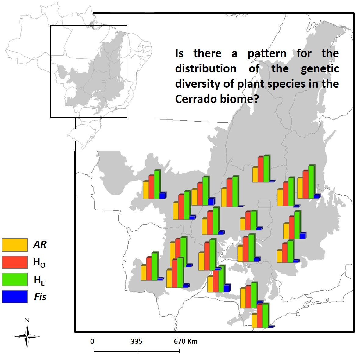
Given this, we propose the hypothesis that the Cerrado plant species have higher genetic diversity and lower inbreeding towards the geographical center of the biome, based on the convention that population size decreases and spatial isolation increases from the center to the periphery of a species’ range, often because of the decreasing quality of habitats toward the edge of the range [19,35]. In this scenario, demographic bottlenecks, varying selection pressures, and restricted gene flow will result in genetic impoverishment, pronounced genetic differentiation among peripheral populations, and substantial divergence from more central populations [34,36,37,38].
Reliable data on the genetic diversity and population structure of species, and the factors that determine their variation within the species’ ranges have proven to be crucial for planning conservation strategies [39]. The value of conservation and the allocation of resources for the preservation of marginal species are still subjects of ample debate [40]. However, it is clear that strong selective pressures caused by stressful conditions can support the acquisitions of new adaptations in marginal areas, conferring a distinct evolutionary potential on these populations [41]. Consequently, our main objective was to evaluate whether the distribution patterns of the genetic diversity of plants in the Cerrado are consistent with the center–periphery model, contributing to understand the population dynamics of these species. Alternatively, concerned with the high fragmentation rate of this biome, we seek to understand whether the genetic variation patterns of native plants can be affected by landscape and climate characteristics, within a conservationist perspective.

2. Materials and Methods

2.1. Literature Search of Genetic Studies on the Vascular Plants of the Cerrado

The data were obtained through an extensive survey of the scientific literature, and for each population (or species) identified, data were obtained on observed heterozygosity (HO), expected heterozygosity (HE), allelic richness (AR), and the inbreeding coefficient (Fis) [42,43], together with the geographical coordinates of the population, thus, the selection of working species depended only on the availability of genetic data. This literature search focused on Scopus, Web of Science, and Scielo databases, which are considered to be the most reliable and comprehensive sources of bibliographic information available online, with Scielo being the standard for Brazilian papers. The search was based on the keywords “SSR (Simple Sequence Repeats) or microsatellite” (according to the method proposed by Vitorino et al. [44]) and “Cerrado”. We chose to use data from microsatellites (nSSRs) because they reflect recent gametic gene flow. Data obtained from the same species, but recovered from different papers were combined for analysis. Species of the same genus, for which we found few population studies, were also combined for analysis. For this combination, we make sure that the combined species have the same life history traits and are therefore subject to similar selective pressures.

2.2. Retrieving Data on Landscape Features

Landscape features were defined using a map of land use and cover of the Cerrado, based on a shapefile available at http://www.dpi.inpe.br/tccerrado/ in 2013 [45]. The map was scanned at a default scale of 1:2,500,000 in ArcGis 10.5 (ESRI), with six classes of land use and cover being recognized (Table 1).
The coordinates obtained for each population (defined by the sampling area) were plotted on the map of the Cerrado, and landscape buffers were created with radii of 1 km, 3 km and 5 km around each population. These buffers were designed to cover the relatively short pollination distances known for some Cerrado species—see [46,47]—and the relatively long distances covered by seed dispersers in this biome [48]. They also provide insights into the possible effects of spatial scale on the observed genetic diversity. The extract by mask tool (in ArcGis) was used to collect the data separately from each buffer, which permitted the identification the relative quantities of the different classes of land use and cover. These quantities were transformed into percentages corresponding to each class. The correlation between classes of variables was assessed using Pearson’s correlation. Variables were excluded from the analysis whenever the correlation was equal to or greater than 0.5 see [49].
Alternatively, the landscape matrix was characterized in the area where each population occurred, because we wanted to know if genetic data were obtained from populations mapped to areas of natural vegetation, pasture, forestry, amongst others.

2.3. Retrieving the Data on Landscape Features

A total of 19 bioclimatic variables were retrieved from the ecoClimate database for analysis in the present study [50]. Variables were chosen for a pre-industrial time-frame (1720–1800) to represent the current climatic conditions, obtained through the atmosphere–ocean general circulation model CCSM4 (CMIP5/PMIP3-http://cmip-pcmdi.llnl.gov/cmip5/ and https://pmip3.lsce.ipsl.fr/). These variables were plotted on a grid of the Neotropical region in cells of 0.5° × 0.5° (longitude vs. latitude), also obtained for each population of climatic data relating to its occurrence cell. Subsequently, the correlation between the variables was also evaluated by Pearson correlation (>0.5) to avoid colinearity. Therefore, only seven of the bioclimatic variables evaluated were maintained (Table 2).

2.4. Spatial Patterns of Genetic Diversity and Structure

Spatially explicit analyses were used to detect central–peripheral patterns in the genetic diversity of the plants evaluated in the present study. This analysis included only species represented by more than three populations. The coordinates of each population were plotted in ArcGis, and the geographical distance (in km) of these populations to the center of the Cerrado was estimated based on a line projected in the editor tool, using the near command. We use a line across the biome to represent the center, considering the longitudinally observed heterogeneity, as it would not be represented by a single geographical point. We chose to evaluate populations in relation to the center of the biome because we were interested in testing whether the instabilities observed at the edge could affect the genetic diversity of populations, since the transition areas are identified as areas of tension see [51]. The relationship between the parameters of genetic diversity (HE, HO, AR, and Fis) and the distance to the centroid of the Cerrado was analyzed using quantile regression [52]. Quantile regression is a way to estimate the conditional quantiles of a response variable distribution in the linear model that provides a more complete view of possible causal relationships between variables in ecological processes.

2.5. Effects of Landscape and Climate on the Genetic Diversity of Cerrado Plants

The effects of landscape features and climatic variables on the HE, HO, AR, and Fis, were evaluated using generalized linear mixed models (GLMM). We used the type of matrix, the percentage of each landscape attribute (remaining vegetation, agriculture) within each buffer, and climatic parameters as the explanatory variables. As the landscape data were collected within a grid of 0.5° × 0.5°, the influence of these variables was evaluated directly through the occurrence of populations in the cells, and not in the buffers. The landscape and the identity of the species were included as random factors, and the explanatory variables as fixed factors, with the construction of the models used being represented by the general equation:
y = + Zu + ε
where y is a N × 1 column vector, the outcome variable;
X is a N × p matrix of the p predictor variables;
β is a p × 1 column vector of the fixed-effects regression coefficients;
Z is the N × q design matrix for the q random effects;
u is a q × 1 vector of the random effects;
and ε is a N × 1 column vector of the residuals.
We also constructed a model to determine whether random effects could also account for the genetic response variables. This model considered the random effects on the identity of the species and the type of landscape matrix only, discarding the effects of climatic variables and landscape attributes. Alternatively, we also consider a general model, which incorporates all the variables considered (full model). The analyses were run in the MCMCglmm package [53] implemented in R 3.6.1 [54], in a Bayesian framework with the Markov Chain Monte Carlo algorithm. We used a total of 80,000 iterations with 20,000 burn-in chains and a Gaussian distribution. We used the Akaike information criteria (AIC) to select the best model, that is, the model with the smallest AICc (the AIC corrected for sample size and the number of parameters), which was considered to be the most plausible for the explanation of the observed patterns [55]. The Delta AICci (ΔAICci, where i represents each model) was calculated as the difference between the AICc for the ith model and the smallest AICc observed. We also determined Akaike’s weight (wAICc), which represents relative contribution of the ith model to the explanation of the observed pattern, given a set of competing models. Models with ΔAICc < 2 were all considered equally plausible as explanations of the observed pattern [56].
We also ran a multiple matrix regression with randomization (MMRR) analysis [57] to evaluate the effects of the geographic distance between pairs of populations and the variation in landscape (e.g., percentage of remnant of native vegetation and agricultural areas), as well as climate differences in the areas where the populations occur on their genetic diversity and inbreeding indices. This analysis was run in the popgenreport package [58].

3. Results

In the present study, literature data were extracted for 31 plant species, totaling 122 populations distributed throughout the Cerrado (Table 3 and Table S1), with overall means of HO = 0.578, HE = 0.684, and AR = 10.018. Low mean genetic diversity was observed in Oryza glumaepatula (HO = 0.078; HE = 0.211; AR = 1.572), Manihot esculenta (HO = 0.315; HE = 0.568; AR = 3.551), Dipteryx alata (HO = 0.333; HE = 0.418; AR = 3.312), and Metrodorea nigra (HO = 0.353; HE = 0.588; AR = 4.000). High inbreeding coefficients were recorded in these species, with the highest values being found in O. glumaepatula (Fis = 0.667), M. esculenta (Fis = 0.435), and M. nigra (Fis = 0.403).
By contrast, the highest genetic diversity values were recorded in Handroanthus chrysotrichus (HO = 0.888; HE = 0.906; AR = 15.000), Annona crassiflora (HO = 0.766; HE = 0.842; AR = 17.650), Tabebuia aurea (HO = 0.765; HE = 0.947; AR = 36.000), and Caryocar brasiliense (HO = 0.764; HO = 0.874; AR = 16.100). Low fixation rates were observed in Plathymenia reticulata (Fis = 0.013), H. chrysotrichus (Fis = 0.021), and Annona coriacea (Fis = 0.022). Negative values were recorded for the fixation index in some species, that is, Solanum lycocarpum (Fis = −0.133), Eugenia dysenterica (Fis = −0.062), Campomanesia adamantium (Fis = −0.030), and Qualea parviflora (Fis = −0.015).

3.1. Spatial Patterns of Genetic Diversity and Structure

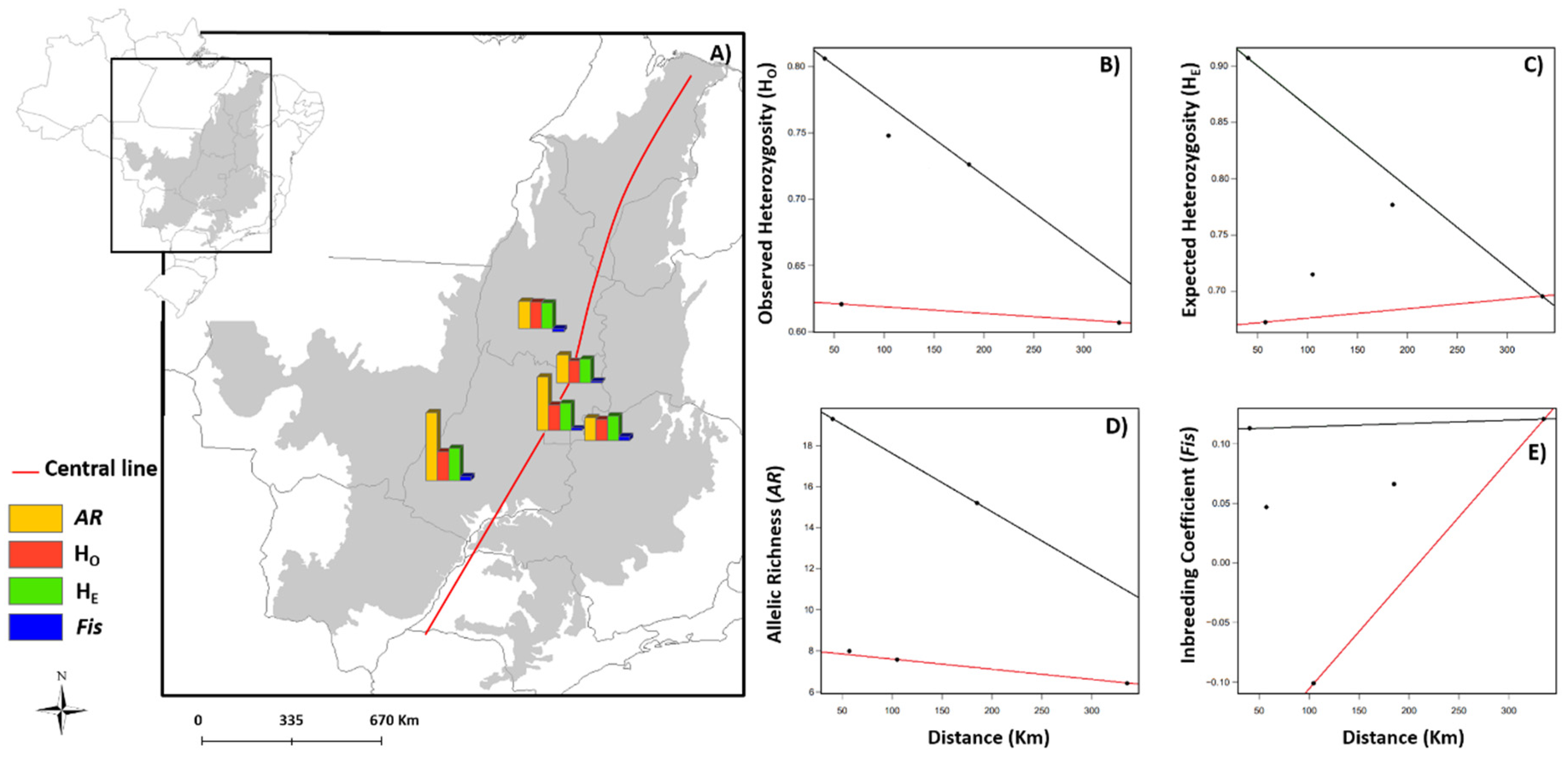
We found a clear center–periphery pattern in the spatial distribution of the genetic parameters in Anonna coriacea and A. crassiflora (Figure 1). The triangular pattern observed for the quantiles reveals that the genetic diversity (HO, HE, and AR) of these species is higher in the center of the biome. As expected, additionally, inbreeding rates (Fis) are higher at the edge of the biome, with reduced genetic diversity in these areas. To visualize the trends and the significance of each regression by species, see Table S2.
In Campomanesia adamantium, we observed higher genetic diversity values (HO, HE, and AR) in the populations located closer to the edge of the biome. Given this, we found lower levels of inbreeding in the edge regions (Figure S1).
In C. langsdorffii, as in Annona, genetic diversity tended to decrease with the increasing distance of the populations from the centroid of the Cerrado and, as expected, higher inbreeding rates were observed in the more outlying populations (Figure S2).
When we analyzed the data on Dimorphandra mollis, we found no clear evidence of a center–periphery pattern and there is a divergence in relation to the quantile 0.99 for HO (Figure S3). For HE, the pattern was consistent with an increase in this index, in populations located closer to the Cerrado border. Thus, a pattern similar to HE was observed for AR and also for Fis.
In the case of the data available on Dipteryx alata, we observed a center–periphery pattern only in HE, that is, the expected heterozygosity showed a tendency to decrease with increasing distance of the populations from the biome’s centroid, which was demonstrated by the 0.99 quantile. The quantiles indicated different patterns for the HO and AR data (Figure S4), although no systematic variation was found in the Fis.
The populations of Eugenia dysenterica presented a clear center-periphery pattern in their genetic diversity, with the HO, HE, and AR values all decreasing with increasing distance of the population from the Cerrado centroid (Figure S5). However, the inbreeding coefficient does not follow the expected pattern, with one quantile showing an increase in the Fis at the edge of the Cerrado, whereas the other reflected a decrease in this coefficient toward the edge of the biome Fis.
A relatively well-defined central–peripheral pattern was also found in the genetic diversity of the Hancornia populations, with the HO and AR values indicating significant structuring of the genetic diversity of these species. This is reflected in the higher inbreeding rates found in the more peripheral populations in the biome (Figure S6).
We analyzed the genera Handroanthus and Tabebuia together, given that their species represent the Tabebuia Alliance clade of Grose and Olmstead [59]. The HO and HE values presented a clear center–periphery pattern, which was reinforced by the higher Fis values observed in the populations at the edge of the Cerrado biome (Figure S7).
We also observed a clear center–periphery pattern in the HE and AR data obtained for Manihot esculenta, although the highest Fis values are highest in the populations located in the center of the biome. While this contradicts the pattern observed in the HE and AR, it is consistent with the HO, which was higher toward the edge of the Cerrado (Figure S8).
The center–periphery pattern was also clear in Oryza glumepatula, with the indices of genetic diversity (HO, HE and AR) decreasing with increasing distance from the center of the biome, while the Fis increased with the increasing distance of the populations, at least to the quantile 0.99 (Figure S9).
By contrast, in the case of the genus Qualea, one quantile indicated a tendency for HO and AR to decrease with increasing distance from the centroid, although this is consistent with the inbreeding coefficient, which tended to be higher in populations over the edge (Figure S10).
In the genus Solanum, we verified a clear center–periphery pattern only in the AR, which decreased with increasing distance from the center of the Cerrado (Figure S11).
We observed a clear center–periphery pattern in the HE and AR of the Vellozia gigantea populations, with genetic diversity decreasing with increasing distance from the Cerrado centroid. However, the inbreeding coefficient also followed this pattern, that is, it decreased with increasing distance from the centroid, which is consistent only with the pattern observed in HO, which increased towards the periphery of the biome (Figure S12).
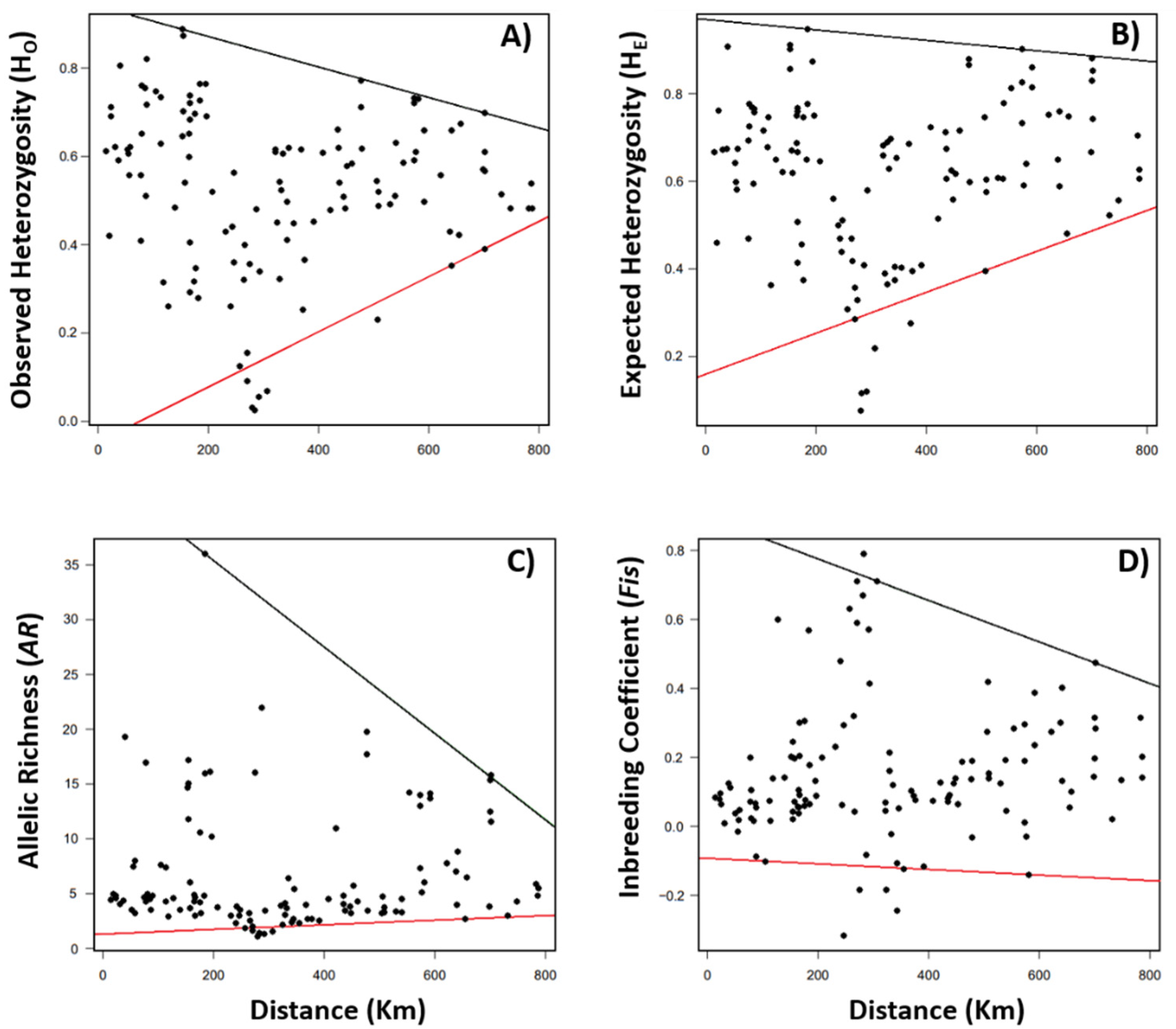
When we analyzed the whole dataset, that is, all the plant species together (Figure 2), we found center–periphery patterns in the HO, HE, and AR values only for the 0.99 quantile. A similar pattern was verified for Fis (0.05 and 0.99).

3.2. Effects of Landscape and Climate on Genetic Diversity

When we analyzed the landscape effects, the models were only significant when we excluded the model that incorporates only the species and landscape matrix. When this model was excluded, the percentage of forestry (FO) in the landscape had a significant effect on the HO patterns in all three buffers, with ∆AICc = 0.0 in all cases, and wAIC = 0.7720 at 1 km, wAIC = 0.6330 at 3 km, and wAIC = 0.6410 at 5 km (Table 4). By contrast, HE was related to the percentage of water (WA) in the 1 km buffer (∆AICc = 0.0; wAIC = 0.9120). The incorporation of WA in the model was also more likely to explain HE in the 3 km buffer (∆AICc = 0.0; wAIC = 0.3300), although in this case, other environmental variables were also capable of explaining the patterns of this index, including VR (∆AICc = 1.3; wAIC = 0.1700), FO (∆AICc = 1.5; wAIC = 0.1590), and AG (∆AICc = 1.6; wAIC = 0.1450). Similarly, for the 5 km buffer, WA provided the best explanation for the observed pattern (∆AICc = 0.0; wAIC = 0.3550), although it was matched by FO (∆AICc = 0.6; wAIC = 0.2680) and AG (∆AICc = 1.7; wAIC = 0.1500).
In the analysis of the landscape effects on the allelic frequency (AR) in the Cerrado plant species, the model that includes the percentage of urban area (UA) best explains the pattern observed in all three buffers, with ∆AICc = 0.0 in all cases, and wAIC = 0.3820 at 1 km, wAIC = 0.3350 at 3 km, and wAIC = 0.3600 at 5 km (Table 5). However, the percentage of water (WA) also had a significant effect on the AR, with ∆AICc = 0.5 and wAIC = 0.3000 at 1 km, ∆AICc = 0.9 and wAIC = 0.2050 at 3 km, and ∆AICc = 0.5 and wAIC = 0.2800 at 5 km (Table 5). In the 1 km buffer, the third most important model was that of pasture (PA), with ∆AICc = 1.4 and wAIC = 0.1930, whereas at 3 km, it was farmland (AG), with ∆AICc = 1.1 and wAIC = 0.1920, and at 5 km, it was forestry (FO), with ∆AICc = 1.3 and wAIC = 0.1920. The inbreeding coefficient (Fis) was most affected by the percentage of FO in the landscape assessed in the 1 km buffer (∆AICc = 0.0 and wAIC = 0.6100), whereas the percentage of UA was the most important variable at 3 km (∆AICc = 0.0; wAIC = 0.6920) and 5 km (∆AICc = 0.0; wAIC = 0.5190).
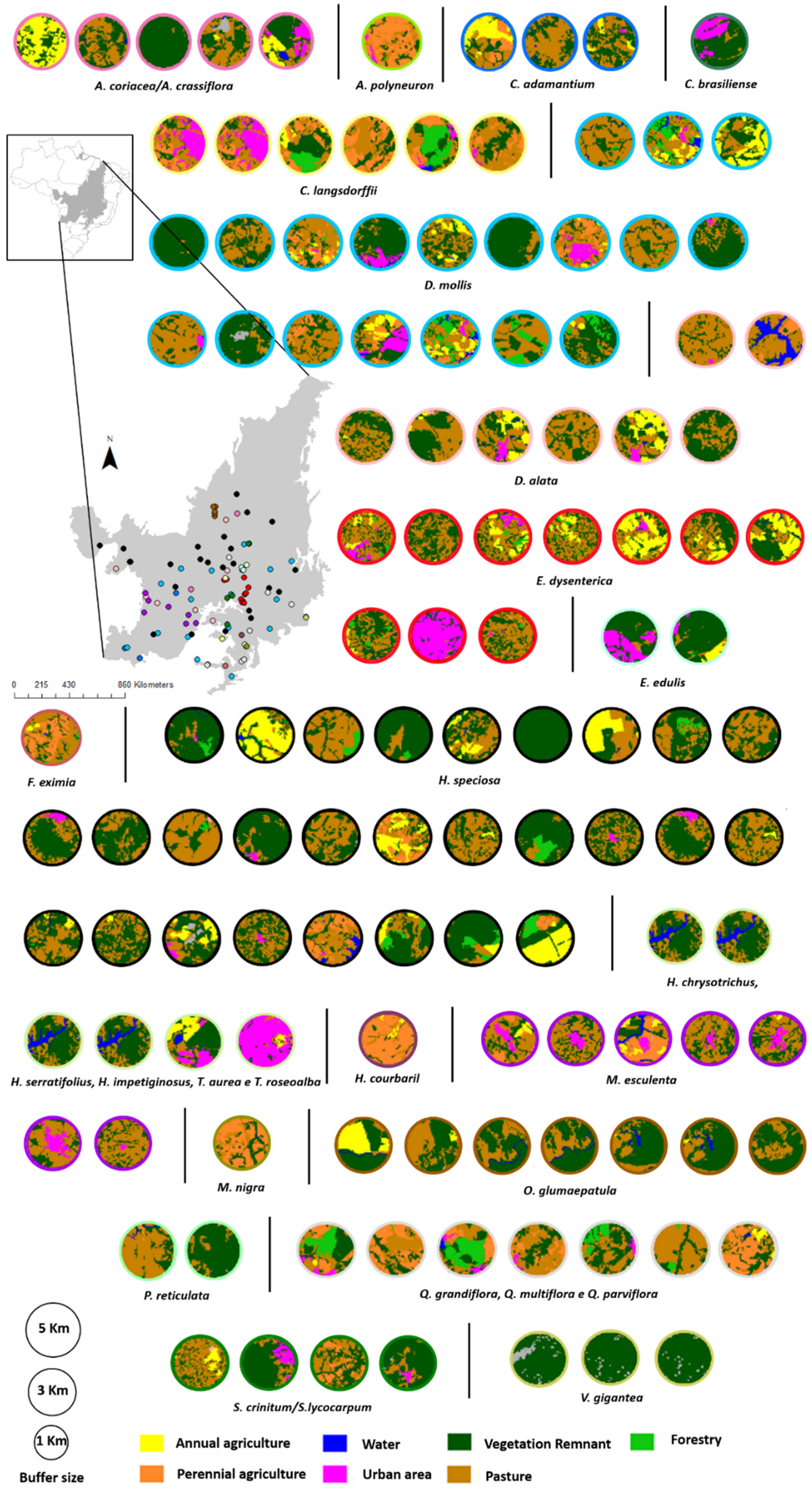
In general, FO, WA, and UA affected the genetic diversity of the plant populations evaluated in the present study (Figure 3). When we related landscape parameters to the genetic diversity data, it was possible to determine that populations with low HO, HE and AR values and high inbreeding coefficients tend to be associated with highly modified landscapes. For example, the populations of O. glumaepatula, are surrounded by a landscape dominated by pasture, while those of M. esculenta occur in areas dominated by urbanization, farmland, and pasture, with few vegetation remnants. A similar pattern was observed in D. alata. In Annona and Handroanthus/Tabebuia, by contrast, high percentages of remnants of natural vegetation were associated with high HO, HE, and AR values.
When we evaluated the effects of the climatic variables associated with the landscape matrix, the mean annual temperature and the isothermality were the principal factors determining the observed genetic patterns. The mean annual temperature MAT has a significant effect on both the HO (∆AICc = 0.0; wAIC = 0.9949) and the HE (∆AICc = 0.0; wAIC = 0.7116), whereas the AR was affected by the combination of all the climate variables analyzed, with ∆AICc = 0.0 and wAIC = 0.7116 (Table 6). The patterns of inbreeding can be accounted for by ISO (∆AICc = 0.0; wAIC = 0.3530), MAT (∆AICc = 0.8; wAIC = 0.2380), and also by the model that incorporates only the species and landscape matrix (∆AICc = 1.3; wAIC = 0.1870).
When we analyzed the influence of the landscape and climatic characters, together with the geographical distance between populations, on the genetic diversity variables, we found that the percentage of WA was the most important variable, in the 1 km buffer, related to the differences in genetic diversity observed among the populations (Table 7). In the 3 km buffer, the geographic distance affected the HO and Fis, although the HE and AR were not influenced by any of the factors analyzed. In the 5 km buffer, geographic distance affected HO and Fis, although the HO was also affected by the percentage of FO, whereas AR was affected by the UA on the landscape. In the case of the climatic variables, the results were similar to those observed in GLMM, that is, the differences observed in the MAT and isothermality (ISO) in the areas occupied by the populations contribute to the variation observed in the genetic diversity.

4. Discussion

The central–peripheral model of genetic diversity was in fact observed in many of the plant species evaluated in the present study, which tended to have higher heterozygosity and allelic richness in the more centrally-located populations, which also tended to have lower levels of inbreeding. This pattern likely reflects a decline in the adaptability of the plants to the abiotic conditions found toward the external limits of the biome. The marginal areas of a species’ range tend to be a zone of transition, where selection pressures are generally more intense [31,60,61]. In this case, species with less phenotypic plasticity will become more stressed physiologically, e.g., [62], which would result in smaller populations, with reduced genetic diversity driven by low gene flow, genetic drift, inbreeding, and directional selection, leading to a marked genetic structure, e.g., [63,64,65,66]. Marginal areas have a number of challenges, including unfavorable abiotic conditions and competition with other species from other biomes [67], and the reduced fitness of the plant may lead to larger fluctuations in population size, reducing effective population size in comparison with larger or more stable populations [68,69,70,71].
The distribution of both Anonna crassiflora and A. coriacea is associated with typical Cerrado environments, that is, nutrient-poor latosols [72]. Hancornia speciosa occurs in the cerrado and cerradão physiognomies, and is thus also associated with poor soils [73], and a similar distribution pattern was observed in E. dysenterica, which inhabits poor, sandy, and acidic soils, predominantly in the Cerrado region and on coastal plains [74]. These preferences, combined with the modifications provoked by the changes in climate occurring during the Pleistocene, have influenced the distribution patterns of these species in the Cerrado biome, in particular, the greater concentration of genetic diversity in the centroid of the biome. Correa Ribeiro et al. [75] concluded that the area to the north of the center of the Cerrado, in the central Goiás highlands, acted as a refuge for the A. coriacea populations during the Pleistocene. Collevatti et al. [76] also showed that a large area of central Brazil, which coincides approximately with the central Cerrado, served as a historical refuge for the H. speciosa populations during long-term climate change.
The patterns observed in the heterozygosity of the Cerrado plant populations were influenced by the matrix in which the populations were located, with the greatest effects being observed in the landscapes dominated by FO, WA, and UA. However, the effect appears to be positive when the natural vegetation is replaced by areas of preservation and restoration of native forests, rather than farmland or pasture. This is consistent with the fact that woody plants, especially fruiting trees, will attract pollinators and dispersers. Pollinators, in particular, will transit between cultivated areas and natural environments [77], and the natural landscape provides an important refuge for a diversity of pollinators which provide pollination services in forestry plantations [78]. Dispersing animals may be attracted to fragments of vegetation close to forestry plantations where they can obtain food. There is also considerable evidence that the crop matrix can provide habitats that support many animal species [79]. These movements of pollinators and dispersers between different habitats within the matrix may thus contribute to the genetic diversity of the plant populations sampled near these areas.
In buffers where the percentage of WA was greater, HE tended to decrease, which is consistent with barrier isolation models. Aquatic environments can create discrete barriers, such as waterfalls and reservoirs, which reduce gene flow between the populations located at their margins, e.g., [80]. However, the river’s slope and the physical–chemical dissimilarities of water can also act as barriers to gene flow and cause detectable differentiation in the genetic constitution of different populations [81,82].
Urban areas also appear to affect the genetic diversity of the plant species evaluated. Some populations sampled in buffers with a high percentage of the urban development presented higher levels of diversity, such as C. brasilienses and T. aurea. Urban areas surrounded by fragments of vegetation can function as barriers to gene flow [83], although they may also facilitate dispersion among populations, leading to greater genetic diversity overall, and reduced differentiation between populations of species that are attracted to urban areas [84]. Many native pollinators, such as bats and bees, may benefit from urban forest resources [85,86], but they usually return to the fragments of native vegetation associated with these areas, thus increasing the flow of pollen between fragments, or even between the urban zone and the fragments. The C. brasilienses populations found in urban areas may be pollinated by the glossophagine bats, Glossophaga soricina and Anoura geoffroyi [87], while T. aurea is pollinated by bees of the genus Centris [88]. These populations can serve as a source of alleles for populations located in fragments of natural vegetation in the area surrounding the urban zone.
Geographical distance affected the variation in the HO and Fis values recorded in the present study, indicating that distance is an important landscape component in the determination of the genetic diversity and structure of plant populations in the Cerrado. These findings are consistent with the previous studies that have verified the occurrence of isolation by the distance between populations of a number of Cerrado plant species, e.g., [89,90,91,92].
The mean annual temperature (MAT) was the principal climatic variable influencing the HO, HE, and Fis, although isothermality (ISO) also affected genetic diversity. Bonte et al. [93] showed that temperature can determine the limits of the geographical ranges of a species, principally by affecting the ability of the plants and juveniles to disperse and become recruited successfully. The gametocytes are especially sensitive to fluctuations in temperature, both during their development, before pollination, and in the post-pollination stage [94]. To avoid negative impacts on their reproduction and physiology [95], plants tend to disperse to regions that correspond to their optimal temperature range [96]. The more central regions of the biomes in which these species occur may encompass this optimal temperature range and other abiotic conditions appropriate for the species, possibly reflecting a relationship between optimal suitability and the typical climatic conditions of the biome. Our model thus supports the hypothesis that current and future climate change will impact the genetic diversity of many plant populations [97,98,99], given that some species, especially those that are already threatened or restricted to habitats created by climate change, are vulnerable to the loss of specific alleles through inbreeding [100]. Combined with climate change, landscape modifications need to be considered carefully in order to guarantee the survival and conservation of the genetic diversity of plant species in Cerrado ecosystems, since they represent the main mechanism for maintaining the food webs.
This study includes patterns for a few species in the Cerrado biome, or even for a few populations of these species, which may be improved in the future, if genetic data for other populations or other plants are available in the literature. Likewise, updated information on land use and land cover in this biome will allow us in the future to establish levels of change at different points in the landscape and assess whether there is a real loss of contemporary gene flow in the most modified areas over time.

5. Conclusions

The distribution of the genetic diversity of many Cerrado plant species follows a typical center–periphery pattern, with greater heterozygosity and lower levels of inbreeding in the populations located more toward the center of the biome. These plants are affected directly by the landscape matrix in which they are located, and in particular by the percentage of forestry cover, water, and urban areas. As modifications to the matrix may affect gene flow, they will ultimately determine the levels of genetic heterozygosity and inbreeding found in a population. The mean annual temperature also influenced genetic diversity in the Cerrado plant species, indicating the influence of the optimal temperature range for the occurrence and genetic diversity of the species. Overall, the results of the study indicate the need for the systematic management of the effects of both changes in climate and shifts in landscape characteristics, in order to minimize the impacts on the genetic diversity of Cerrado plant species.

Supplementary Materials

The following are available online at https://0-www-mdpi-com.brum.beds.ac.uk/1424-2818/12/11/421/s1, Table S1: Species or subspecies, number of microsatellite locus and reference article used to obtain the genetic parameters: Observed Heterozygosity (HO), Expected Heterozygosity (HE), Allelic Richness (AR), and inbreeding coefficients (Fis) for Cerrado plant populations. Figure S1: Distribution of genetic diversity indices and the inbreeding coefficient for the Campomanesia adamantium populations sampled in the Cerrado biome. Figure S2: Distribution of the genetic diversity indices and inbreeding coefficients of the Copaifera langsdorffii populations sampled in the Cerrado biome. Figure S3: Distribution of the genetic diversity indices and inbreeding coefficients for the Dimorphandra mollis populations sampled in the Cerrado biome. Figure S4: Distribution of genetic diversity indices and inbreeding coefficients of the populations of Dipteryx alata sampled in the Cerrado biome. Figure S5: Distribution of the genetic diversity and inbreeding coefficients of the Eugenia dysenterica populations sampled in the Cerrado biome. Figure S6: Distribution of the genetic diversity indices and the inbreeding coefficients of the populations of Hancornia speciosa cuyabensis, Hancornia speciosa gardinerii, Hancornia speciosa pubescens, and Hancornia speciosa speciosa sampled in the Cerrado biome. Figure S7: Distribution of the genetic diversity indices and inbreeding coefficients of the populations of Handroanthus chrysotrichus, Handroanthus serratifolius, Handroanthus impetiginosus, Tabebuia aurea, and Tabebuia roseoalba sampled in the Cerrado biome. Figure S8: Distribution of the genetic diversity indices and inbreeding coefficients of the of Manihot esculenta populations sampled in the Cerrado biome. Figure S9: Distribution of the genetic diversity indices and inbreeding coefficients of the Oryza glumaepatula populations sampled in the Cerrado biome. Figure S10: Distribution of the genetic diversity indices and inbreeding coefficients off the populations of Qualea grandflora, Qualea multiflora, and Qualea parviflora sampled in the Cerrado biome. Figure S11: Distribution of the genetic diversity indices and inbreeding coefficients for the populations of Solanum crinitum and Solanum lycocarpum sampled in the Cerrado biome. Figure S12: Distribution of the genetic diversity indices and inbreeding coefficients recorded in the populations of Vellozia gigantea sampled in the Cerrado biome. Table S2: Values referring to parameter β (b1) and significance (P) obtained in quantile regressions (quantiles 0.05 and 0.99) relating genetic diversity data, Observed Heterozygosity (HO), Expected Heterozygosity (HE), Allelic Richness (AR), and inbreeding coefficients (Fis) and distance (km) of plant species populations, in relation to the center of the Cerrado biome.

Author Contributions

Conceptualization, L.C.V.; methodology, L.C.V.; formal analysis, M.N.O.R.; resources, M.N.O.R. and U.J.B.d.S.; writing—original draft preparation, L.C.V. and M.N.O.R.; writing—review and editing, L.A.B.; supervision, U.J.B.d.S.; project administration, F.G.S. All authors have read and agreed to the published version of the manuscript.

Funding

This research received no external funding.

Acknowledgments

The authors are grateful to the Foundation de Amparo à Pesquisa do Estado de Goiás (Goiás State Research Foundation, FAPEG) and the Rio Verde Campus of the Federal Institute Goiano, for the infrastructure and the students involved in this study.

Conflicts of Interest

The authors declare that they have no known competing financial interests or personal relationships that could have appeared to influence the work reported in this paper.

References

  1. Andeson, C.D.; Eppeeson, B.K.; Fortin, M.-J.; Holderegger, F.; James, P.M.A.; Rosenberg, M.S.; Scribner, K.T.; Spear, S. Considering spatial and temporal scale in landscape-genetic studies of gene flow. Mol. Ecol. 2010, 19, 3565–3575. [Google Scholar] [CrossRef]
  2. Cushman, S.A.; Shirk, A.; Landguth, E.L. Separating the effects of habitat area, fragmentation and matrix resistance on genetic differentiation in complex landscapes. Landsc. Ecol. 2012, 27, 369–380. [Google Scholar] [CrossRef]
  3. Holderegger, R.; Di Giulio, M. The genetic effects of roads: A review of empirical evidence. Basic Appl. Ecol. 2010, 11, 522–531. [Google Scholar] [CrossRef]
  4. Kamm, U.; Gugerli, F.; Rotach, P.; Edwards, P.; Holderegger, R. Open areas in a landscape enhance pollen-mediated gene flow of a tree species: Evidence from northern Switzerland. Landsc. Ecol. 2010, 25, 903–911. [Google Scholar] [CrossRef] [Green Version]
  5. Leimu, R.; Vergeer, P.; Angeloni, F.; Ouborg, N.J. Habitat fragmentation, climate change, and inbreeding in plants. Ann. N. Y. Acad. Sci. 2010, 1195, 84–98. [Google Scholar] [CrossRef] [PubMed]
  6. Ezard, T.H.G.; Travis, J.M.J. The impact of habitat loss and fragmentation on genetic drift and fixation time. Oikos 2006, 114, 367–375. [Google Scholar] [CrossRef]
  7. Brook, B.W.; Sodhi, N.S.; Bradshaw, C.J. Synergies among extinction drivers under global change. Trends Ecol. Evol. 2008, 23, 453–460. [Google Scholar] [CrossRef] [PubMed]
  8. Pujol, B.; Blanchet, S.; Charmantier, A.; Danchin, E.; Facon, B.; Marrot, P.; Roux, F.; Scotti, I.; Teplitsky, C.; Thomson, C.E.; et al. The missing response to selection in the wild. Trends Ecol. Evol. 2018, 33, 337–346. [Google Scholar] [CrossRef] [PubMed] [Green Version]
  9. Keller, L.F.; Waller, D.M. Inbreeding effects in wild populations. Trends Ecol. Evol. 2002, 17, 230–241. [Google Scholar] [CrossRef]
  10. Reed, D.H.; Frankham, R. Correlation between fitness and genetic diversity. Conserv. Biol. 2003, 17, 230–237. [Google Scholar] [CrossRef]
  11. Berec, L.; Angulo, E.; Courchamp, F. Multiple Allee effects and population management. Trends Ecol. Evol. 2007, 22, 185–191. [Google Scholar] [CrossRef]
  12. Strassburg, B.B.N.; Brooks, T.; Feltran-Barbieri, R.; Iribarrem, A.; Crouzeilles, R.; Loyola, R.; Latawiec, A.E.; Oliveira, F.F.J.B.; Scaramuzza, C.A.M.; Scarano, F.R.; et al. Moment of truth for the Cerrado hotspot. Nat. Ecol. Evol. 2017, 1, 0099. [Google Scholar] [CrossRef]
  13. Gibbs, P.E.; Leitão Filho, H.D.F.; Shepherd, G. Floristic composition and community structure in an area of cerrado in SE Brazil. Flora 1983, 173, 433–449. [Google Scholar] [CrossRef]
  14. Sano, E.E.; Rosa, R.; Brito, J.L.S.; Ferreira, L.G. Land cover mapping of the tropical savanna region in Brazil. Environ. Monit. Assess. 2010, 166, 113–124. [Google Scholar] [CrossRef]
  15. Spera, S.A.; Galford, G.L.; Coe, M.T.; Macedo, M.N.; Mustard, J.F. Land-use change affects water recycling in Brazil’s last agricultural frontier. Glob. Chang. Biol. 2016, 22, 3405–3413. [Google Scholar] [CrossRef]
  16. Latrubesse, E.M.; Arima, E.; Ferreira, M.E.; Nogueira, S.H.; Wittmann, F.; Dias, M.S.; Dagosta, F.C.P.; Bayer, M. Fostering water resource governance and conservation in the Brazilian Cerrado biome. Conserv. Sci. Pract. 2019, 1, e77. [Google Scholar] [CrossRef] [Green Version]
  17. Myers, N.; Mittermeier, R.A.; Mittermeier, C.G.; da Fonseca, G.A.B.; Kent, J. Biodiversity hotspots for conservation priorities. Nature 2010, 403, 853–858. [Google Scholar] [CrossRef]
  18. Leidner, A.K.; Haddad, N.M. Combining measures of dispersal to identify conservation strategies in fragmented landscapes. Conserv. Biol. 2011, 25, 1022–1031. [Google Scholar] [CrossRef]
  19. Aguilar, R.; Quesada, M.; Ashworth, L.; Herrerias-Diego, Y.; Lobo, J. Genetic consequences of habitat fragmentation in plant populations: Susceptible signals in plant traits and methodological approaches. Mol. Ecol. 2008, 17, 5177–5188. [Google Scholar] [CrossRef]
  20. Diniz-Filho, J.A.F.; Nabout, J.C.; Bini, L.M.; Soares, T.N.; Telles, M.P.C.; Marco, P., Jr.; Collevatti, R.G. Niche modelling and landscape genetics of Caryocar brasiliense (“Pequi” tree: Caryocaraceae) in Brazilian Cerrado: An integrative approach for evaluating central–peripheral population patterns. Tree Genet. Genomes 2009, 5, 617–627. [Google Scholar] [CrossRef]
  21. Collevatti, R.G.; Telles, M.P.C.; Nabout, J.C.; Chaves, L.J.; Soares, T.N. Demographic history and the low genetic diversity in Dipteryx alata (Fabaceae) from Brazilian Neotropical savannas. Heredity 2013, 111, 97–105. [Google Scholar] [CrossRef] [Green Version]
  22. Eidesen, P.B.; Ehrich, D.; Bakkestuen, V.; Alsos, I.G.; Gilg, O.; Taberlet, P.; Brochmann, C. Genetic roadmap of the Arctic: Plant dispersal highways, traffic barriers and capitals of diversity. New Phytol. 2013, 200, 898–910. [Google Scholar] [CrossRef] [Green Version]
  23. Gwitira, I.; Murwira, A.; Shekede, M.D.; Masocha, M.; Chapano, C. Precipitation of the warmest quarter and temperature of the warmest month are key to understanding the effect of climate change on plant species diversity in Southern African savannah. Afr. J. Ecol. 2014, 52, 209–216. [Google Scholar] [CrossRef]
  24. Collevatti, R.G.; Nabout, J.C.; Diniz-Filho, J.A.F. Range shift and loss of genetic diversity under climate change in Caryocar brasiliense, a Neotropical tree species. Tree Genet. Genomes 2011, 7, 1237–1247. [Google Scholar] [CrossRef]
  25. Taberlet, P.; Fumagalli, L.; Wust-Saucy, A.G.; Cosson, J.F. Comparative phylogeography and postglacial colonization routes in Europe. Mol. Ecol. 1998, 7, 453–464. [Google Scholar] [CrossRef]
  26. Soltis, D.E.; Morris, A.B.; McLachlan, J.S.; Manos, P.S.; Soltis, P.S. Comparative phylogeography of unglaciated eastern North America. Mol. Ecol. 2006, 15, 4261–4293. [Google Scholar] [CrossRef]
  27. Stewart, J.R. The progressive effect of the individualistic response of species to Quaternary climate change: An analysis of British mammalian faunas. Quat. Sci. Rev. 2008, 27, 2499–2508. [Google Scholar] [CrossRef] [Green Version]
  28. Edwards, D.L.; Keogh, J.S.; Knowles, L.L. Effects of vicariant barriers, habitat stability, population isolation and environmental features on species divergence in the south-western Australian coastal reptile community. Mol. Ecol. 2012, 21, 3809–3822. [Google Scholar] [CrossRef] [Green Version]
  29. Collevatti, R.G.; Lima, N.E.; Vitorino, L.V. The diversification of extant angiosperms in the South American dry diagonal. In Neotropical Diversification: Patterns and Processes; Rull, V., Carnaval, A.C., Eds.; Springer: Berlin/Heidelberg, Germany, 2020; pp. 547–567. [Google Scholar]
  30. Sagarin, R.D.; Gaines, S.D. The ‘abundant centre’ distribution: To what extent is it a biogeographical rule? Ecol. Lett. 2002, 5, 137–147. [Google Scholar] [CrossRef]
  31. Eckert, C.G.; Samis, K.E.; Lougheed, S.C. Genetic variation across species’ geographical ranges: The central–marginal hypothesis and beyond. Mol. Ecol. 2008, 17, 1170–1188. [Google Scholar] [CrossRef]
  32. Gaston, K.J. Geographic range limits: Achieving synthesis. Proc. R. Soc. B 2009, 276, 1395–1406. [Google Scholar] [CrossRef] [Green Version]
  33. Pironon, S.; Villellas, J.; Morris, W.F.; Doak, D.F.; García, M.B. Do geographic, climatic or historical ranges differentiate the performance of central versus peripheral populations? Glob. Ecol. Biogeogr. 2015, 24, 611–620. [Google Scholar] [CrossRef]
  34. Pironon, S.; Papuga, G.; Villellas, J.; Angert, A.L.; García, M.B.; Thompson, J.D. Geographic variation in genetic and demographic performance: New insights from an old biogeographical paradigm. Biol. Rev. 2017, 92, 1877–1909. [Google Scholar] [CrossRef]
  35. Hampe, A.; Petit, R.J. Conserving biodiversity under climate change: The rear edge matters. Ecol. Lett. 2005, 8, 461–467. [Google Scholar] [CrossRef] [Green Version]
  36. Jones, B.; Gliddon, C.; Good, J.E.G. The conservation of variation in geographically peripheral populations: Lloydia serotina (Liliaceae) in Britain. Biol. Conserv. 2001, 101, 147–156. [Google Scholar] [CrossRef]
  37. Barrett, S.C.; Ness, R.W.; Vallejo-Marín, M. Evolutionary pathways to self-fertilization in a tristylous plant species. New Phytol. 2009, 183, 546–556. [Google Scholar] [CrossRef] [PubMed]
  38. Ortego, J.; Riordan, E.C.; Gugger, P.F.; Sork, V.L. Influence of environmental heterogeneity on genetic diversity and structure in an endemic southern Californian oak. Mol. Ecol. 2012, 21, 3210–3223. [Google Scholar] [CrossRef]
  39. Lesica, P.; Allendorf, F.W. When are peripheral populations valuable for conservation? Conserv. Biol. 1995, 9, 753–760. [Google Scholar] [CrossRef]
  40. Moretti, M.; Caretti, P.; Bricalli, A.; Andrello, M. Genetic diversity and reproductive ecology of the sage-leaved rockrose, Cistus salviifolius L., in the Swiss Alps. Plant Ecol. 2020, 221, 361–374. [Google Scholar] [CrossRef]
  41. Morente-López, J.; Kass, J.M.; Lara-Romero, C.; Serra-Diaz, J.M.; Soto-Correa, J.C.; Anderson, P.; Iriondo, J.M. Ecological niche models as hypothesis generators of functional genetic differentiation and potential local adaptation in a Mediterranean alpine ecosystem. bioRxiv 2020. [Google Scholar] [CrossRef]
  42. Nei, M. Molecular Evolutionary Genetics, 1st ed.; Columbia University Press: New York, NY, USA, 1987; p. 512. [Google Scholar]
  43. Nei, M.; Kumar, S. Molecular Evolution and Phylogenetics, 1st ed.; Oxford University Press: New York, NY, USA, 2000; p. 333. [Google Scholar]
  44. Vitorino, L.C.; Souza, U.J.B.; Jardim, T.P.F.A.; Ballesteros-Mejia, L. Towards inclusion of genetic diversity measures into IUCN assessments: A case study on birds. Anim. Biodiv. Conserv. 2019, 42, 317–335. [Google Scholar] [CrossRef]
  45. MMA, IBAMA, EMBRAPA, INPE, UFG, UFU Terra Class Cerrado—Mapeamento Do Uso e Cobertura da Terra Do Cerrado. Available online: http://www.dpi.inpe.br/tccerrado/download.php (accessed on 4 February 2020).
  46. Collevatti, R.G.; Estolano, R.; Garcia, S.F.; Hay, J.D. Short-distance pollen dispersal and high self-pollination in a bat-pollinated neotropical tree. Tree Genet. Genomes 2010, 6, 555–564. [Google Scholar] [CrossRef]
  47. Almeida-Júnior, E.B.; Collevatti, R.G.; Telles, M.P.D.C.; Chaves, L.J.; Neres, D.F.; Soares, T.N. Short-distance pollen dispersal in a protogynous Annonaceae tree species from the Brazilian Cerrado. Plant Syst. Evol. 2018, 304, 1091–1099. [Google Scholar] [CrossRef]
  48. Fragoso, J.M.; Silvius, K.M.; Correa, J.A. Long-distance seed dispersal by tapirs increases seed survival and aggregates tropical trees. Ecology 2003, 84, 1998–2006. [Google Scholar] [CrossRef]
  49. Bonate, P.L. The effect of collinearity on parameter estimates in nonlinear mixed effect models. Pharm. Res. 1999, 16, 709–717. [Google Scholar] [CrossRef]
  50. Lima-Ribeiro, M.S.; Varela, S.; González-Hernández, J.; Oliveira, G.; Diniz-Filho, J.A.F.; Terribile, L.C. EcoClimate: A database of climate data from multiple models for past, present, and future for macroecologists and biogeographers. Biodivers. Inform. 2015, 10, 1–21. [Google Scholar] [CrossRef] [Green Version]
  51. Gosz, J.R.; Sharpe, P.J.H. Broad-scale concepts for interactions of climate, topography, and biota at biome transitions. Landsc. Ecol. 1989, 3, 229–243. [Google Scholar] [CrossRef]
  52. Cade, B.S.; Noon, B.R. A gentle introduction to quantile regression for ecologists. Front. Ecol. Environ. 2003, 1, 412–420. [Google Scholar] [CrossRef]
  53. Hadfield, J.D. MCMC methods for multi-response generalized linear mixed models: The MCMCglmm R package. J. Stat. Softw. 2010, 33, 1–22. [Google Scholar] [CrossRef] [Green Version]
  54. R Core Team. A Language and Environment for Statistical Computing; R Foundation for Statistical Computing: Vienna, Austria, 2019; Available online: https://cran.rproject.org/bin/windows/base/old/3.5.3/ (accessed on 4 February 2020).
  55. Burnham, K.P.; Anderson, D.R. Model Selection and Multimodel Inference, 2nd ed.; Springer: New York, NY, USA, 2002. [Google Scholar]
  56. Zuur, A.; Ieno, E.N.; Walker, N.; Saveliev, A.A.; Smith, G.M. Mixed Effects Models and Extensions in Ecology with R; Springer Science & Business Media: Berlin/Heidelberg, Germany, 2009. [Google Scholar]
  57. Wang, I.J. Examining the full effects of landscape heterogeneity on spatial genetic variation: A multiple matrix regression approach for quantifying geographic and ecological isolation. Evolution 2013, 67, 3403–3411. [Google Scholar] [CrossRef] [PubMed]
  58. Adamack, A.T.; Gruber, B. PopGenReport: Simplifying basic population genetic analyses in R. Methods Ecol. Evol. 2014, 5, 384–387. [Google Scholar] [CrossRef]
  59. Grose, S.O.; Olmstead, R.G. Taxonomic Revisions in the Polyphyletic Genus Tabebuia s. I. (Bignoniaceae). Syst. Bot. 2007, 33, 660–670. [Google Scholar] [CrossRef]
  60. Hamilton, J.A.; Eckert, C.G. Population genetic consequences of geographic disjunction: A prairie plant isolated on Great Lakes alvars. Mol. Ecol. 2007, 16, 1649–1660. [Google Scholar] [CrossRef]
  61. Pulliam, H.R. On the relationship between niche and distribution. Ecol. Lett. 2020, 3, 349–361. [Google Scholar] [CrossRef]
  62. Zinn, K.E.; Tunc-Ozdemir, M.; Harper, J.F. Temperature stress and plant sexual reproduction: Uncovering the weakest links. J. Exp. Bot. 2010, 61, 1959–1968. [Google Scholar] [CrossRef] [Green Version]
  63. Braasch, J.; Barker, B.S.; Dlugosch, K.M. Expansion history and environmental suitability shape effective population size in a plant invasion. Mol. Ecol. 2019, 28, 2546–2558. [Google Scholar] [CrossRef] [PubMed]
  64. Lázaro-Nogal, A.; Matesanz, S.; García-Fernández, A.; Traveset, A.; Valladares, F. Population size, center-periphery, and seed dispersers’ effects on the genetic diversity and population structure of the Mediterranean relict shrub Cneorum Tricoccon. Ecol Evol. 2017, 7, 7231–7242. [Google Scholar] [CrossRef] [Green Version]
  65. Arnaud-Haond, S.; Teixeira, S.; Massa, S.I.; Billot, C.; Saenger, P.; Coupland, G.; Serrao, E.A. Genetic structure at range edge: Low diversity and high inbreeding in Southeast Asian mangrove (Avicennia marina) populations. Mol. Ecol. 2006, 15, 3515–3525. [Google Scholar] [CrossRef]
  66. Gapare, W.J.; Aitken, S.N. Strong spatial genetic structure in peripheral but not core populations of Sitka spruce [Picea sitchensis (Bong.) Carr.]. Mol. Ecol. 2005, 14, 2659–2667. [Google Scholar] [CrossRef]
  67. Françoso, R.D.; Haidar, R.F.; Machado, R.B. Tree species of South America central savanna: Endemism, marginal areas and the relationship with other biomes. Acta Bot. Bras. 2016, 30, 78–86. [Google Scholar] [CrossRef] [Green Version]
  68. Crow, J.F.; Morton, N.E. Measurement of gene frequency drift in small populations. Evolution 1955, 9, 202–214. [Google Scholar] [CrossRef]
  69. Frankham, R. Relationship of genetic variation to population size in wildlife. Conserv. Biol. 1996, 10, 1500–1508. [Google Scholar] [CrossRef] [Green Version]
  70. Kimura, M.; Crow, J.F. The measurement of effective population number. Evolution 1963, 17, 279–288. [Google Scholar] [CrossRef]
  71. Wright, S. Size of population and breeding structure in relation to evolution. Science 1938, 87, 430–431. [Google Scholar]
  72. Mesquita, M.A.M.; Naves, R.V.; Souza, E.R.B.; Bernardes, T.G.; Silva, L.B. Caracterização de ambientes com alta ocorrência natural de araticum (Annona crassiflora Mart.) no estado de Goiás. Rev. Bras. Frutic. 2007, 29, 15–19. [Google Scholar] [CrossRef]
  73. Silva, R.S.M.; Chaves, L.J.; Naves, R.V. Caracterização de frutos e árvores de cagaita (Eugenia dysenterica DC.) no sudeste do Estado de Goiás, Brasil. Rev. Bras. Frutic. 2001, 23, 330–334. [Google Scholar] [CrossRef] [Green Version]
  74. Vieira, N.R.D.; da Silva, J.J.F.; Ledo, A.; da Mangaba, S. Fruticultura Tropical: Espécies Regionais e Exóticas; dos Santos Serejo, J.A., Dantas, J.L.L., Coelho, C.V.S., Coelho, Y.d.S., Eds.; Embrapa Informação Tecnológica: Brasilia/Distrito Federal, Brasil, 2009; pp. 323–338. [Google Scholar]
  75. Correa, R.P.; Lemos-Filho, J.P.; de Oliveira, B.R.S.; Lovato, M.B.; Heuertz, M. Species-specific phylogeographical patterns and Pleistocene east–west divergence in Annona (Annonaceae) in the Brazilian Cerrado. Bot. J. Linn. Soc. 2016, 181, 21–36. [Google Scholar] [CrossRef] [Green Version]
  76. Collevatti, R.G.; Rodrigues, E.E.; Vitorino, L.C.; Lima-Ribeiro, M.S.; Chaves, L.J.; Telles, M.P. Unravelling the genetic differentiation among varieties of the Neotropical savana tree Hancornia speciosa Gomes. Ann. Bot. 2018, 122, 973–984. [Google Scholar] [CrossRef] [PubMed]
  77. Cunningham-Minnick, M.J.; Peters, V.E.; Crist, T.O. Bee communities and pollination services in adjacent crop fields following flower removal in an invasive forest shrub. Ecol. Appl. 2020, 30, e02078. [Google Scholar] [CrossRef]
  78. Tscharntke, T.; Klein, A.M.; Kruess, A.; Steffan-Dewenter, I.; Thies, C. Landscape perspectives on agricultural intensification and biodiversity–ecosystem service management. Ecol. Lett. 2005, 8, 857–874. [Google Scholar] [CrossRef]
  79. Prevedello, J.A.; Almeida-Gomes, M.; Lindenmayer, D.B. The importance of scattered trees for biodiversity conservation: A global meta-analysis. J. Appl. Ecol. 2018, 55, 205–214. [Google Scholar] [CrossRef]
  80. Gonçalves, F.R.; Vieira, F.A.; Carvalho, D. Naturally fragmented but not genetically isolated populations of Podocarpus sellowii Klotzsch (Podocarpaceae) in southeast Brazil. Genet. Mol. Res. 2016, 15, 1–17. [Google Scholar] [CrossRef] [PubMed]
  81. Beheregaray, L.B.; Cooke, G.M.; Chao, N.L.; Landguth, E.L. Ecological speciation in the tropics: Insights from comparative genetic studies in Amazonia. Front. Genet. 2015, 5, 477. [Google Scholar] [CrossRef] [Green Version]
  82. Cook, B.D.; Kennard, M.J.; Real, K.; Pusey, B.J.; Hughes, J.M. Landscape genetic analysis of the tropical freshwater fish Mogurnda mogurnda (Eleotridae) in a monsoonal river basin: Importance of hydrographic factors and population history. Freshw. Biol. 2011, 56, 812–827. [Google Scholar] [CrossRef]
  83. Sebbenn, A. Effects of forest fragmentation on the effective and realized gene flow of Neotropical tree species: Implications for genetic conservation. BMC Proc. 2011, 5, 6. [Google Scholar] [CrossRef] [Green Version]
  84. Miles, L.S.; Rivkin, L.R.; Johnson, M.T.J.; Munshi-South, J.; Verrelli, B.C. Gene flow and genetic drift in urban environments. Mol. Ecol. 2019, 28, 4138–4151. [Google Scholar] [CrossRef]
  85. Nascimento, V.T.; Agostini, K.; Souza, C.S.; Maruyama, P.K. Tropical urban areas support highly diverse plant-pollinator interactions: An assessment from Brazil. Landsc. Urban Plan. 2020, 198, 103801. [Google Scholar] [CrossRef]
  86. Diniz, U.M.; Lima, S.A.; Machado, I.C. Short-distance pollen dispersal by bats in an urban setting: Monitoring the movement of a vertebrate pollinator through fluorescent dyes. Urban Ecosyst. 2019, 22, 281–291. [Google Scholar] [CrossRef]
  87. Gribel, R.; Hay, J.D. Pollination ecology of Caryocar brasiliense (Caryocaraceae) in Central Brazil cerrado vegetation. J. Trop. Ecol. 1993, 9, 199–211. [Google Scholar] [CrossRef]
  88. Barros, M.G. Pollination ecology of Tabebuia aurea (Manso) Benth. & Hook. and T. ochracea (Cham.) Standl. (Bignoniaceae) in Central Brazil cerrado vegetation. Rev. Bras. Bot. 2001, 24, 255–261. [Google Scholar] [CrossRef]
  89. Fava, W.S.; da Costa, P.C.; Lorenz, A.P. Ecological niche modelling and genetic analyses reveal lack of geographic differentiation of Leptolobium dasycarpum (Leguminosae, Papilionoideae) across the Brazilian savannah. Flora 2020, 264, 151566. [Google Scholar] [CrossRef]
  90. Diniz-Filho, J.A.F.; Soares, T.N.; Lima, J.S.; Dobrovolski, R.; Landeiro, V.L.; Telles, M.P.D.C.; Bini, L.M. Mantel test in population genetics. Genet. Mol. Biol. 2013, 36, 475–485. [Google Scholar] [CrossRef] [Green Version]
  91. Zucchi, M.I.; Brondani, R.P.V.; Pinheiro, J.B.; Chaves, L.J.; Coelho, A.S.G.; Vencovsky, R. Genetic structure and gene flow in Eugenia dysenterica DC in the Brazilian Cerrado utilizing SSR markers. Genet. Mol. Biol. 2003, 26, 449–457. [Google Scholar] [CrossRef] [Green Version]
  92. Batistini, A.P.; Telles, M.P.D.C.; Bertoni, B.W.; Coppede, J.D.S.; Môro, F.V.; Pereira, A.M.S.; França, S.D.C. Genetic diversity of natural populations of Anemopaegma arvense (Bignoniaceae) in the Cerrado of São Paulo State, Brazil. Genet. Mol. Res. 2009, 8, 52–63. [Google Scholar] [CrossRef]
  93. Bonte, D.; Travis, J.M.; De Clercq, N.; Zwertvaegher, I.; Lens, L. Thermal conditions during juvenile development affect adult dispersal in a spider. Proc. Natl. Acad. Sci. USA 2008, 105, 17000–17005. [Google Scholar] [CrossRef] [Green Version]
  94. Hedhly, A. Sensitivity of flowering plant gametophytes to temperature fluctuations. Environ. Exp. Bot. 2011, 74, 9–16. [Google Scholar] [CrossRef] [Green Version]
  95. Dusenge, M.E.; Duarte, A.G.; Way, D.A. Plant carbon metabolism and climate change: Elevated CO2 and temperature impacts on photosynthesis, photorespiration and respiration. New Phytol. 2019, 221, 32–49. [Google Scholar] [CrossRef] [Green Version]
  96. Grace, J. Climatic tolerance and the distribution of plants. New Phytol. 1987, 106, 113–130. [Google Scholar] [CrossRef]
  97. Pauls, S.U.; Nowak, C.; Bálint, M.; Pfenninger, M. The impact of global climate change on genetic diversity within populations and species. Mol. Ecol. 2013, 22, 925–946. [Google Scholar] [CrossRef] [PubMed]
  98. Kramer, K.; Degen, B.; Buschbom, J.; Hickler, T.; Thuiller, W.; Sykes, M.T.; de Winter, W. Modelling exploration of the future of European beech (Fagus sylvatica L.) under climate change—Range, abundance, genetic diversity and adaptive response. For. Ecol. Manag. 2010, 259, 2213–2222. [Google Scholar] [CrossRef]
  99. Doi, H.; Takahashi, M.; Katano, I. Genetic diversity increases regional variation in phenological dates in response to climate change. Glob. Chang. Biol. 2010, 16, 373–379. [Google Scholar] [CrossRef]
  100. Dubey, S.; Pike, D.A.; Shine, R. Predicting the impacts of climate change on genetic diversity in an endangered lizard species. Clim. Chang. 2013, 117, 319–327. [Google Scholar] [CrossRef] [Green Version]
Figure 1. Indices of genetic diversity and inbreeding recorded for the populations of Anonna coriacea and Anonna crassiflora sampled in the Cerrado biome (A). Central line is the line that defines the latidudinal center of the biome. Quantile regression for the relationships between the observed (HO) and expected Heterozygosity (HE), allelic richness (AR), and inbreeding coefficient (Fis) and the distance from the Cerrado centroid. Figures (BE) show the triangle-shaped quantile fits from 0.05 (red line) to 0.99 (black line).
Diversity 12 00421 g001
Figure 2. Distribution of the genetic diversity indices and inbreeding coefficients for populations of all the plants sampled in the Cerrado biome. Quantile regression for the relationships between the observed (HO) and expected heterozygosity (HE), allelic richness (AR), and inbreeding coefficient (Fis), and the distance from the centroid of the Cerrado. Figures (AD) show the triangle-shaped envelopes of the 0.05 (red line) and 0.99 (black line) quantile fits.
Diversity 12 00421 g002
Figure 3. Distribution of the plant populations evaluated in the present study in the Cerrado biome and the percentages of the different land use and cover categories observed with the landscape buffers established around the different populations. Points of the same color on the population distribution map indicate populations of the same species. Points that have the same color as the external line of the buffer, represent the signalled species. The circles represent the observed landscape for the 5 km buffer, which were reduced according to the scale, to obtain the data for 3 km and 1 km.
Diversity 12 00421 g003
Table 1. Classes of land use and cover used to model the genetic diversity of Cerrado plant species in the present study.
ClassAbbreviationDescription
AgricultureAGFarmland planted with annual or perennial crops
WaterWANatural or artificial bodies of water
Urban areaUAAreas of urban development
Vegetation RemnantVRRemnant areas of native vegetation
PasturePAAreas of cattle ranching, with no arboreal vegetation
ForestryFOAreas of preservation and restoration of native forests
Table 2. Bioclimatic variables used to model the genetic diversity of the Cerrado plants analyzed in the present study.
VariableCodeDescription
Bio 01—Mean Annual TemperatureMAT
Bio 03—IsothermalityISO(Mean Diurnal Range/BIO7) (* 100)
Bio 07—Annual Temperature RangeATR(Max Temperature of Warmest Month–Min Temperature of Coldest Month)
Bio 09—Mean Temperature of Driest QuarterTDQ
Bio 12—Annual PrecipitationAP
Bio 15—Precipitation SeasonalityPS(Coefficient of Variation)
Bio 18—Precipitation of the Warmest QuarterPWQ
/ Division sign and * Multiplication sign.
Table 3. Mean observed heterozygosity (HO), expected heterozygosity (HE) (mean within population genetic diversity), allelic richness (AR), and inbreeding coefficients (Fis) recorded in the Cerrado plant species surveyed in the present study.
Species or SubspeciesNumber of IndividualsNumber of PopulationsHOHEARFis
Annona coriacea Mart.5530.6580.6967.3330.022
Annona crassiflora Mart.10420.7660.84217.650.089
Aspidosperma polyneuron Müll.Arg.3010.4300.6507.0600.301
Campomanesia adamantium (Cambess.) O.Berg20730.5860.5635.333−0.030
Caryocar brasiliense A.St.-Hil.10110.7640.87416.1000.131
Copaifera langsdorffii Desf.88660.6970.87315.9750.205
Dimorphandra mollis Benth.157190.4390.5893.6520.255
Dipteryx alata Vogel16680.3330.4183.3120.208
Eugenia dysenterica DC.127100.4580.4273.128−0.062
Euterpe edulis Mart.88320.6930.74810.4000.075
Ficus eximia Schott.6010.7110.87917.7500.191
Hancornia speciosa var. cuyabensis Malme16450.5910.6894.0200.144
Hancornia speciosa var. gardinerii (A.DC.) Müll.Arg.379140.6390.7004.2720.090
Hancornia speciosa var. pubescens (Nees & Mart.) Müll.Arg.14660.6820.7374.6430.078
Hancornia speciosa var. speciosa9730.6040.6774.1630.099
Handroanthus chrysotrichus (Mart. ex DC.) Mattos9810.8880.90615.0000.021
Handroanthus serratifolius
(Vahl) S.O.Grose
10810.6460.85717.2000.245
Handroanthus impetiginosus (Mart. ex DC.) Mattos7510.7030.85711.8000.199
Hymenaea courbaril L.24110.5860.81314.2000.284
Manihot esculenta Crantz21970.3150.5683.5510.435
Metrodorea nigra A.St.-Hil.4010.3530.5884.0000.403
Oryza glumaepatula Steud.19570.0780.2111.5720.667
Plathymenia reticulata Benth.11120.7290.7397.3880.013
Qualea grandiflora Mart.50050.5410.79412.1200.320
Qualea multiflora Mart.2010.5780.6185.7500.064
Qualea parviflora Mart.2010.6070.5987.500−0.015
Solanum crinitum Lam.12020.4430.49214.0000.099
Solanum lycocarpum A.St.-Hil.12020.4180.36819.000−0.133
Tabebuia aurea (Silva Manso) Benth. & Hook.f. ex S.Moore26010.7650.94736.0000.178
Tabebuia roseoalba (Ridl.) Sandwith69020.7160.83111.3000.158
Vellozia gigantea N.L.Menezes & Mello-Silva2430.5000.6455.3980.220
Mean ± SD206.55 ± 230.353.903 ± 4.1900.578 ± 0.1700.684 ± 0.17610.018 ± 7.2350.159 ± 0.161
Table 4. Models used to test the hypothesis of the influence of landscape features, that is, the percentage of agriculture (AG), water (WA), urban areas (UA), remnant vegetation (RV), pasture (PA), and forest (FO), on the observed (HO) and expected heterozygosity (HE) recorded in 121 plant populations in the Cerrado biome of central Brazil. Analyses were run using 1 km, 3 km and 5 km buffers. The models with ∆AICc < 2.0 are highlighted in bold type. AICc = AIC corrected by sample size and number of parameters in the model; wAIC = Akaike weight.
Model∆AICcwAICKβp
1 km
HO vs. Species + FO + Matrix0.00.772060.021-
HO vs. Species + WA + Matrix3.30.003760.0151.000
HO vs. Species + AG + Matrix6.7<0.00160.0121.000
HO vs. Species + VR + Matrix7.3<0.00160.0151.000
HO vs. Species + UA + Matrix7.6<0.00160.0011.000
HO vs. Species + PA + Matrix8.2<0.00160.0161.000
HO vs. Full Model68.2<0.001110.0120.432
3 km
HO vs. Species + FO + Matrix0.00.633060.022-
HO vs. Species + WA + Matrix2.40.169060.0191.000
HO vs. Species + VR + Matrix4.40.001560.0251.000
HO vs. Species + AG + Matrix4.6<0.00160.0221.000
HO vs. Species + UA + Matrix5.8<0.00160.0231.000
HO vs. Species + PA + Matrix6.1<0.00160.0221.000
HO vs. Full Model64.9<0.001110.0150.231
5 km
HO vs. Species + FO + Matrix0.00.641060.001-
HO vs. Species + WA + Matrix2.70.163060.0001.000
HO vs. Species + AG + Matrix3.80.095060.0021.000
HO vs. Species + PA + Matrix5.70.037060.0021.000
HO vs. Species + UA + Matrix6.00.033060.0001.000
HO vs. Species + VR + Matrix6.00.031060.0031.000
HO vs. Full Model62.9<0.001110.0010.321
Model∆AICcwAICKβp
1 km
HE vs. Species + WA + Matrix0.00.91206−0.0020.000
HE vs. Species + PA + Matrix7.30.00236−0.0050.000
HE vs. Species + AG + Matrix7.80.00196−0.0020.000
HE vs. Species + UA + Matrix7.90.00186−0.0070.000
HE vs. Species + FO + Matrix8.20.00156−0.007-
HE vs. Species + VR + Matrix8.60.00136−0.0020.000
HE vs. Full Model69.2<0.00111−0.0050.026
3 km
HE vs. Species + WA + Matrix0.00.33006−0.0020.000
HE vs. Species + VR + Matrix1.30.17006−0.0050.000
HE vs. Species + FO + Matrix1.50.15906−0.002-
HE vs. Species + AG + Matrix1.60.14506−0.0070.000
HE vs. Species + UA + Matrix2.20.10906−0.0070.000
HE vs. Species + PA + Matrix2.70.08706−0.0020.000
HE vs. Full Model65.0<0.00111−0.0050.122
5 km
HE vs. Species + WA + Matrix0.00.35506−0.0740.000
HE vs. Species + FO + Matrix0.60.26806−0.063-
HE vs. Species + AG + Matrix1.70.15006−0.0631.000
HE vs. Species + UA + Matrix2.10.12206−0.0720.000
HE vs. Species + VR + Matrix3.60.05806−0.0621.000
HE vs. Species + PA + Matrix4.00.04706−0.0691.000
HE vs. Full Model64.1<0.00111−0.0770.345
Legend: K = number of parameters that consider the β of the explanatory variables and the distribution parameters of the residuals.
Table 5. Models used to test the hypothesis of the influence of landscape features, that is, the percentage of agriculture (AG), water (WA), urban areas (UA), remnant vegetation (RV), pasture (PA), and forestry (FO), on the allelic richness (AR) and inbreeding coefficient (Fis) recorded in 121 plant populations in the Cerrado biome of central Brazil. Analyses were run using 1 km, 3 km and 5 km buffers. The models with ∆AICc < 2.0 are highlighted in bold type. AICc = AIC corrected by sample size and number of parameters in the model; wAIC = Akaike weight.
Model∆AICcwAICKβp
1 km
AR vs. Species + UA + Matrix0.00.382060.6920.000
AR vs. Species + WA + Matrix0.50.300060.7400.000
AR vs. Species + PA + Matrix1.40.193060.8350.000
AR vs. Species + AG + Matrix4.10.004960.6610.000
AR vs. Species + FO + Matrix4.30.004560.683-
AR vs. Species + VR + Matrix5.00.003160.7160.000
AR vs. Full Model40.1<0.001110.8690.088
3 km
AR vs. Species + UA + Matrix0.00.33506−0.1690.000
AR vs. Species + WA + Matrix0.90.205060.0710.000
AR vs. Species + AG + Matrix1.10.19206−0.0540.000
AR vs. Species + PA + Matrix2.20.109060.0500.000
AR vs. Species + FO + Matrix2.30.103060.016-
AR vs. Species + VR + Matrix3.20.067060.0290.000
AR vs. Full Model37.0<0.00111−0.1840.108
5 km
AR vs. Species + UA + Matrix0.00.36006−0.3170.000
AR vs. Species + WA + Matrix0.50.28006−0.3541.000
AR vs. Species + FO + Matrix1.30.19206−0.152-
AR vs. Species + AG + Matrix3.30.06906−0.3590.000
AR vs. Species + PA + Matrix3.50.06206−0.1640.000
AR vs. Species + VR + Matrix4.50.03806−0.2141.000
AR vs. Full Model31.3<0.00111−0.2011.000
Model∆AICcwAICKβp-Value
1 km
Fis vs. Species + FO + Matrix0.00.61006−0.029-
Fis vs. Species + WA + Matrix2.90.14606−0.0031.000
Fis vs. Species + UA + Matrix3.40.00236−0.0241.000
Fis vs. Species + PA + Matrix3.80.00176−0.0221.000
Fis vs. Species + AG + Matrix6.7<0.0016−0.0311.000
Fis vs. Species + VR + Matrix6.9<0.0016−0.0291.000
Fis vs. Full Model65.7<0.00111−0.0170.321
3 km
Fis vs. Species + UA + Matrix0.00.692060.0480.000
Fis vs. Species + FO + Matrix3.00.156060.059-
Fis vs. Species + WA + Matrix5.00.005860.0621.000
Fis vs. Species + PA + Matrix5.2<0.00160.0551.000
Fis vs. Species + VR + Matrix6.7<0.00160.0641.000
Fis vs. Species + AG + Matrix7.2<0.00160.0621.000
Fis vs. Full Model62.4<0.001110.0440.061
5 km
Fis vs. Species + UA + Matrix0.00.51906−0.0360.000
Fis vs. Species + FO + Matrix2.20.17406−0.030-
Fis vs. Species + PA + Matrix2.60.13906−0.0280.000
Fis vs. Species + WA + Matrix2.80.12906−0.0261.000
Fis vs. Species + AG + Matrix6.40.02206−0.0281.000
Fis vs. Species + VR + Matrix6.70.01806−0.0301.000
Fis vs. Full Model58.6<0.00111−0.0370.055
Legend: K = number of parameters that consider the β of the explanatory variables and the distribution parameters of the residuals.
Table 6. Models used to test the hypothesis of the influence climatic parameters, that is, the mean annual temperature (MAT), isothermality (ISO), annual temperature range (ATR), mean temperature of driest quarter (TDQ), annual precipitation (AP), precipitation seasonality (PS), and precipitation of the warmest quarter (PWQ), on the observed (HO) and expected heterozygosity (HE), the allelic richness (AR), and the inbreeding coefficient (Fis) recorded in 121 plant populations in the Cerrado biome of central Brazil. Analyses were run using 1 km, 3 km and 5 km buffers. The models with ∆AICc < 2.0 are highlighted in bold type. AICc = AIC corrected by sample size and number of parameters in the model; wAIC = Akaike weight.
Model∆AICcwAICKβp
HO vs. Species + MAT + Matrix0.00.994960.0030.000
HO vs. Species + PWQ + Matrix12.90.001660.0030.002
HO vs. Species + PS + Matrix13.30.001360.0060.025
HO vs. Species + TDQ + Matrix13.8<0.00160.0050.002
HO vs. Species + Matrix14.4<0.00150.001-
HO vs. Species + ISO + Matrix16.4<0.00160.0000.348
HO vs. Species + ATR + Matrix17.6<0.00160.0010.456
HO vs. Species + AP + Matrix20.3<0.00160.0010.920
HO vs. Full Model24.1<0.001120.0000.000
HE vs. Species + MAT + Matrix0.00.71166−0.0010.005
HE vs. Species + Matrix3.40.131850.006-
HE vs. Species + PS + Matrix5.10.055760.0000.136
HE vs. Species + ISO + Matrix6.30.030860.0060.965
HE vs. Species + ATR + Matrix7.00.021760.0080.628
HE vs. Species + TDQ + Matrix7.10.021060.0000.020
HE vs. Species + PWQ + Matrix7.50.01676−0.0020.059
HE vs. Species + AP + Matrix9.20.007360.0080.665
HE vs. Full Model25.0<0.00112−0.0040.087
AR vs. Full Model0.00.711612−1.0880.005
AR vs. Species + PS + Matrix13.20.13186−0.8260.036
AR vs. Species + MAT + Matrix13.60.05576−0.9450.037
AR vs. Species + PWQ + Matrix14.70.03086−1.0330.010
AR vs. Species + ISO + Matrix15.40.02176−0.9900.317
AR vs. Species + ATR + Matrix16.40.02106−0.9160.331
AR vs. Species + AP + Matrix18.30.01676−0.8740.269
AR vs. Species + TDQ + Matrix19.00.00736−0.9040.059
Ra vs. Species + Matrix19.3<0.0015−0.9310.068
Fis vs. Species + ISO + Matrix0.00.353012−0.0120.049
Fis vs. Species + MAT + Matrix0.80.23806−0.0060.036
Fis vs. Species + Matrix1.30.18706−0.0140.037
Fis vs. Species + ATR + Matrix2.90.08106−0.0110.187
Fis vs. Species + PS + Matrix3.20.07106−0.0110.204
Fis vs. Species + AP + Matrix4.40.04016−0.0170.115
Fis vs. Species + PWQ + Matrix5.30.02506−0.0030.075
Fis vs. Species + TDQ + Matrix8.50.00056−0.0110.268
Fis vs. Full Model21.2<0.0015−0.0050.167
Legend: K = number of parameters that consider the β of the explanatory variables and the distribution parameters of the residuals.
Table 7. Models tested by the multiple matrix regression with randomization (MMRR), based on the hypothesis that the geographic distance (Geo distance) between populations, landscape parameters (agriculture, AG; water, WA; urban areas, UA; remnant vegetation, RV; pasture, PA, and forestry, FO), and the climatic variables, that is, mean annual temperature (MAT), isothermality (ISO), annual temperature range (ATR), mean temperature of driest quarter (TDQ), annual precipitation (AP), precipitation seasonality (PS), and precipitation of the warmest quarter (PWQ), account for the pattern of variation observed in the genetic diversity (HO, HE), allelic richness (AR), and the inbreeding coefficient (Fis) in 121 plant populations in the Cerrado biome. The analyses were run using buffers of 1 km, 3 km, and 5 km.
Landscape—1 km
HOHEARFis
pR2 pR2 pR2 pR2
Intercept0.910.083Intercept0.7880.038Intercept0.4940.030Intercept0.9930.109
Geo distance0.2630.007Geo distance0.8330.077Geo distance0.0470.246Geo distance0.0570.006
AG0.8900.083AG0.5800.038AG0.8350.028AG0.0540.109
WA0.0010.007WA0.0300.077WA0.7990.246WA0.0070.006
UA0.6230.083UA0.3890.038UA0.9780.028UA0.1710.109
PA0.6140.007PA0.0390.077PA0.9330.246PA0.4300.006
VR0.5790.082VR0.4740.038VR0.0030.028VR0.0350.109
FO0.2720.007FO0.9490.077FO0.0900.246FO0.0950.006
Landscape—3 km
pR2 pR2 pR2 pR2
Intercept0.5050.023Intercept0.3080.014Intercept0.5920.034Intercept0.7360.019
Geo distance0.0450.248Geo distance0.6180.504Geo distance0.1430.191Geo distance0.0260.503
AG0.2550.024AG0.7150.014AG0.4820.034AG0.8930.020
WA0.1780.248WA0.0760.504WA0.3040.191WA0.6590.503
UA0.8790.023UA0.9620.014UA0.0600.034UA0.9890.020
PA0.7070.248PA0.7010.504PA0.5110.191PA0.2220.503
VR0.1910.024VR0.1030.014VR0.6990.034VR0.1980.020
FO0.0950.248FO0.6390.504FO0.0730.191FO0.5850.503
Landscape—5 km
pR2 pR2 pR2 pR2
Intercept0.1750.038Intercept0.1730.023Intercept0.6490.060Intercept0.4780.023
Geo distance0.0340.079Geo distance0.4150.215Geo distance0.2110.051Geo distance0.0210.400
AG0.1780.038AG0.6610.023AG0.1880.060AG0.8270.023
WA0.1420.079WA0.0570.215WA0.1910.051WA0.5070.400
UA0.6510.038UA0.8770.023UA0.0310.060UA0.3970.023
PA0.1720.079PA0.0530.215PA0.7990.051PA0.1570.400
VR0.1910.038VR0.1650.023VR0.5100.060VR0.3090.023
FO0.0330.079FO0.2070.215FO0.3330.051FO0.6350.400
Climate
pR2 pR2 pR2 pR2
Intercept0.8850.038Intercept0.8860.024Intercept0.8590.064Intercept1.0000.048
Geo distance0.3450.018Geo distance0.3820.076Geo distance0.0090.015Geo distance0.2310.018
TDQ0.0050.038TDQ0.1720.024TDQ0.6460.064TDQ0.1730.048
PWQ0.0540.018PWQ0.7570.076PWQ0.0460.015PWQ0.0150.018
PS0.1620.038PS0.9010.024PS0.6580.064PS0.6420.048
AP0.2230.018AP0.2040.076AP0.3700.015AP0.4740.018
ATR0.5270.038ATR0.6750.024ATR0.1920.064ATR0.5070.048
MAT0.0010.018MAT0.0020.076MAT0.0260.015MAT0.0040.018
ISO0.9500.038ISO0.3100.024ISO0.0010.064ISO0.0150.048
Publisher’s Note: MDPI stays neutral with regard to jurisdictional claims in published maps and institutional affiliations.

