Effects of Temperature Rise on Multi-Taxa Distributions in Mountain Ecosystems


1
Biodiversity Monitoring Office, Gran Paradiso National Park, Via Pio VII 9, 10135 Turin, Italy
2
Management and Conservation of Natural Resources Office, Ossola Protected Areas, Viale Pieri 27, 28868 Varzo (VB), Italy
3
Institute of Geosciences and Earth Resources, National Research Council, Via Moruzzi 1, 56124 Pisa, Italy
*
Author to whom correspondence should be addressed.
Diversity 2020, 12(6), 210; https://0-doi-org.brum.beds.ac.uk/10.3390/d12060210
Submission received: 22 April 2020
/
Revised: 18 May 2020
/
Accepted: 21 May 2020
/
Published: 26 May 2020
(This article belongs to the Special Issue Biodiversity of Insect)
Abstract
:Mountain biodiversity is associated with rare and fragile biota that are highly sensitive to climate change. To estimate the vulnerability of biodiversity to temperature rise, long-term field data are crucial. Species distribution models are an essential tool, in particular for invertebrates, for which detailed information on spatial and temporal distributions is largely missing. We applied presence-only distribution models to field data obtained from a systematic survey of 5 taxa (birds, butterflies, carabids, spiders, staphylinids), monitored in the northwestern Italian Alps. We estimated the effects of a moderate temperature increase on the multi-taxa distributions. Only small changes in the overall biodiversity patterns emerged, but we observed significant differences between groups of species and along the altitudinal gradient. The effects of temperature increase could be more pronounced for spiders and butterflies, and particularly detrimental for high-altitude species. We observed significant changes in community composition and species richness, especially in the alpine belt, but a clear separation between vegetation levels was retained also in the warming scenarios. Our conservative approach suggests that even a moderate temperature increase (about 1 °C) could influence animal biodiversity in mountain ecosystems: only long-term field data can provide the information to improve quantitative predictions, allowing us to readily identify the most informative signals of forthcoming changes.
1. Introduction
Climate change is driving community composition rearrangements and biodiversity losses worldwide, currently representing a crucial theme in conservation biology (e.g., [1,2,3]). Understanding and predicting global warming impacts on biodiversity is essential to develop effective conservation strategies (e.g., [4,5]).
Not all ecosystems display the same degree of exposure, sensitivity, and vulnerability [3,6]. Mountain ecosystems host a high level of biodiversity and are especially threatened (e.g., [7]), owing to the presence of species with small distribution areas, low dispersal ability, and high levels of physiological and ecological specialization [8,9,10]. In the European Alps, a large number of endemic species is present, and during the last decades, many habitat types and animal and plant populations have undergone exceptional decline [11,12,13]. Many mountain ecosystems reported warming higher than the global average [14,15,16,17]: in the Italian Alps, the measured air temperature rise was of the order of 0.2–0.4 °C per decade since 1950 [18,19]. For the Alps, climate projections suggest future warming of 0.5–0.7 °C per decade [20], again higher than the global average [21,22].
Alpine biodiversity has already responded to the temperature rise. For alpine flora, common effects are upward displacements of high altitude plants, treeline advance, the decline of arctic-alpine species, changes in community composition, and species richness (e.g., [11,13,23,24,25]). For alpine fauna, similar responses have been measured, such as upward shifts of single species and changes at assemblage level [26,27,28,29], but the number of studies is markedly lower.
Individual species are expected to respond differently to climate warming, and the most important effects will presumably be at the community level [1,30]. Even though the temperature rise has been reported to impact community composition, the number of long-term standardized datasets with a sufficiently high temporal and spatial resolution is still limited, in particular for multi-taxa analyses [31,32,33].
Understanding how multiple species and communities will respond to climate change is essential for management, from global to local scale [34,35]. Indeed, the effectiveness of protected areas and of the Natura 2000 network under climate change has been questioned (e.g., [3,36,37]). It has been argued that nature reserves should improve their role from pure conservation to the stewardship of the changes, representing key sites for the study of climate change responses [38,39]. Conservation actions should consequently include the management of “smoother transitions” to new conditions, which necessarily requires the understanding of current dynamics and future states [39].
Species distribution models (SDM) are simple tools to estimate taxa response to climate warming, assessing the potential vulnerability of individual species and communities as a whole [40,41,42,43]. SDM could have large uncertainties in their outcomes, as they use a correlative approach based on the observed, realized species niche. SDM usually assume niche conservatism and the absence of evolutionary processes, ignoring biological interactions and physiological mechanisms [44,45]. More sophisticated, mechanistic models are currently available, but they have high data demands and thus cannot be used for any of the studied taxa, owing to the lack of data (e.g., [46,47]). Consequently, simple SDM are often considered as the main tool to estimate species and community vulnerability to climate change [40,48] and fill knowledge gaps in understudied taxa and habitats (e.g., invertebrates, [31,49]; altitudinal gradients and mountain ecosystems, [50,51]). SDM allows us to explore different scenarios and quantify biodiversity changes for a wide range of species at the same time, obtaining useful indications for protected areas’ management [5,39,40].
To obtain quantitative information on biodiversity along altitudinal gradients on spatial and temporal scales suitable for site management, a multi-taxa monitoring project was started in 2007 in the northwestern Italian Alps [52]. Five taxa (Coleoptera Carabidae, Coleoptera Staphylinidae, Araneae, Lepidoptera Papilionoidea and Hesperiioidea, Aves) representing a wide array of ecological and evolutionary traits, have been monitored in three separated mountain protected areas. Climatic and vegetation data were collected on the same spatial scales. The results of the analyses have shown that invertebrate species’ richness and community composition are related to temperature and altitude, highlighting the potential vulnerability of the alpine communities to climate change [52,53].
The present work uses the above dataset to assess the risk of short-term changes in Alpine animal biodiversity under climate warming. The coarse spatial resolution of current (global and regional) climate projections, however, does not allow to assess the response of mountain ecosystems, that are characterized by high topographic heterogeneity and small-scale microhabitat and microclimate variability [54,55]. Short-term, fine-grained climate predictions would certainly be needed by site managers [56], but there is still a generalized paucity of climate information for mountain areas [57].
On the other hand, it is important to provide informative projections, even within simplified modeling exercises, to investigate the relationships between land-use and climate change [58,59]. Our study, based on local-scale biodiversity and environmental data, is a contribution to address the challenge of estimating the response of multi-taxa distributions. We applied “what if” scenarios, increasing the maximum, minimum, and mean temperatures with respect to the increase observed in the Alps during the last decades. To assess the potential role of land cover, we compared projections with and without vegetation constraints.
Many works indicate differences in the ability of different taxa to adapt to climate change, but most of the studies are based on meta-analysis or data coming from independent studies [33,56,60]. Our approach compared data coming from different taxa collected with the same methodologies and in the same monitoring framework. Our main objective was thus to estimate patterns of congruence in multi-taxa response to climate warming. In particular, we asked whether: (i) the number of species changing their distribution differs among taxa, degree of vulnerability and scenarios and (ii) species richness and community composition significantly change along the altitudinal gradient. This allowed us to obtain indications on both indicator selection and habitat protection priorities.
2. Materials and Methods
2.1. Biodiversity Inventory in the Northwestern Italian Alps: Data Sources
In 2007, 3 protected areas in the NW Italian Alps (Gran Paradiso National Park, Orsiera Rocciavré Natural Park, Veglia Devero Natural Park) started monitoring animal biodiversity along altitudinal gradients. Twelve altitudinal transects have been identified (overall covered elevational range 550–2700 m), each characterized by 5–7 sampling units spaced apart by an altitudinal range of 200 m, for a total of 69 plots (circular areas with 100 m radius). Plot characteristics and their spatial locations are detailed in the Supplementary Material (Table S1).
Five taxa have been monitored in 2007, using semi-quantitative methods. Carabids (Coleoptera Carabidae), staphylinids (Coleoptera Staphylinidae), and spiders (Arachnida Araneae) were monitored through pitfall traps (5 per plot, filled by 10 cc of white vinegar, checked every 15 days from May to September). Butterflies (Lepidoptera Papilionoidea and Hesperiioidea) were monitored through linear transects (200 m along one of the diameters of each plot, once per month from May to September). Birds (Aves) were monitored through point counts (lasting 20 min, twice per plot between April and July, choosing the most appropriate period depending on altitude). We refer to [52] for a detailed description of the sampling methodology. Butterflies were mainly identified in the field, and only a few specimens were collected for subsequent identification in the laboratory. Epigeic invertebrates (Carabidae, Staphylinidae, Araneae) were identified in the laboratory by expert taxonomists and are currently stored at the park’s headquarters.
These taxa were selected because they are good candidates for estimating biodiversity patterns along altitudinal gradients [61,62,63,64]. In particular, they are: (i) well represented in mountain ecosystems, both in terms of species richness and number of individuals, and (ii) characterized by species with different ecological needs and different levels of specialization. Altogether, the selected taxa include different trophic levels and different taxonomic relatedness. Moreover, they can all be sampled using easy-to-apply, cheap, standardized, and well-established techniques, that allow monitoring repeatability through space and time.
To characterize microclimatic conditions at the plot scale, we installed one data-logger (iButton, DS1922, Maxim, Sunnyvale, CA, USA) at the center of each plot, at about 1 m above ground, recording hourly air temperature from June to September. We calculated mean, maximum, minimum, and standard deviation of daily temperature at each plot and averaged them to obtain seasonal values. Each plot was described by: (i) mean altitude; (ii) geographic position (a categorical variable indicating which protected area they belong to); (iii) vegetation belt (Montane, Subalpine, Alpine, indicating altitudinal sections characterized by given vegetation and climate, [65,66]); (iv) structural diversity. To obtain structural diversity, we empirically estimated during field surveys, using 5% classes and checking vegetation maps, the percentage of ground covered by different structural layers (herbaceous layer, low shrubs < 1 m, tall shrubs between 1–5 m, trees, stone, and bare ground cover). We then calculated structural diversity as the Shannon index of the herbaceous layer, shrub, and tree cover. This index quantifies microhabitat heterogeneity, and it is often adopted in conservation studies (e.g., [52,67,68]).
2.2. Model Simulation: Current Conditions and Temperature Change Scenarios
We applied Species Distribution Models to 304 species (45 carabids, 40 staphylinids, 99 spiders, 80 butterflies, 40 birds), using distribution data coming from 62 plots. Indeed, 7 plots have been discarded owing to missing temperature records and 359 species were present in less than 4 plots (selected as a threshold for presence accuracy). Each of the 304 species, as shown in Table S2a, was characterized by: (i) the taxon they belong to; (ii) the degree of vulnerability (a dichotomous variable indicating if the species is restricted to high altitude); (iii) the level of endemism (a dichotomous variable indicating if the species is endemic of the Alpine biogeographical region).
We modeled each species individually and subsequently estimated species richness and community metrics on model outputs that were converted to presence/absence data, following the approach “predict-first, assemble later”, or stacked species distribution models [34]. This approach implies unsaturation at the community level, which is currently considered a very likely assumption [69], and allowed us to create unconstrained species richness and community composition maps.
To create species distribution models, we used Maxent, a machine-learning approach based on maximum entropy (Maxent software 3.3), developed by S. Phillips and colleagues ([70], freely available at http://www.cs.princeton.edu/~schapire/maxent).
We selected Maxent because it is a high-performing and robust bioclimatic approach, widely used in recent years [71,72,73]. In particular, Maxent (i) can be run with both continuous and categorical variables [71]; (ii) it is stable also with correlated predictors [71], and consequently we were allowed to simultaneously model the effects of temperature and altitude; and (iii) it is highly trustworthy with a reduced number of presences [74,75,76], consequently allowing modeling also of rare and endemic species [77,78,79].
The species distribution is modeled by comparing environmental conditions at plots where the species is present with the conditions encountered across the study area. These latter are defined by a set of background points that identify the available environment. For each plot, Maxent estimates the probability distribution that best fits the environmental conditions at the plot, remaining as close as possible to a uniform distribution (maximum entropy principle). For each plot, a logistic output is then generated. This can be interpreted as an estimate of the presence probability, given the environment, with values ranging from 0 (lowest probability) to 1 (highest probability) (see [70,71,80] for a detailed explanation of methodology). We used the default parameterization of Maxent regarding feature types, regularization, and prevalence [74,81].
We selected for both the sample plots and the background points the same 62 monitored plots, to limit our predictions to a set of sampling units for which all data were collected at the same scale. Several works indicate in fact that macro- (coarse-scale air conditions) and micro-climate (experienced by organisms) can be significantly different, in particular in mountain ecosystems. Consequently, it is microclimate that should be used in SDM [82,83]. The role of microhabitat associations in determining current and future distributions of living organisms has also been emphasized [84]. As environmental predictors, we thus chose the variables measured in each plot that define local microclimate, altitude, geographical location, and vegetation cover (microhabitat).
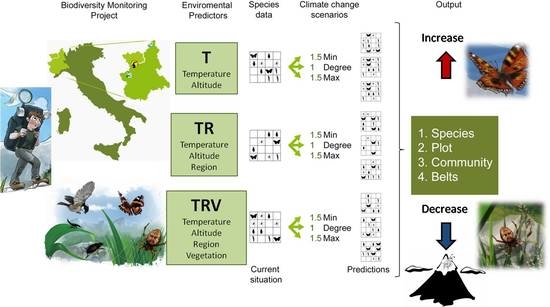
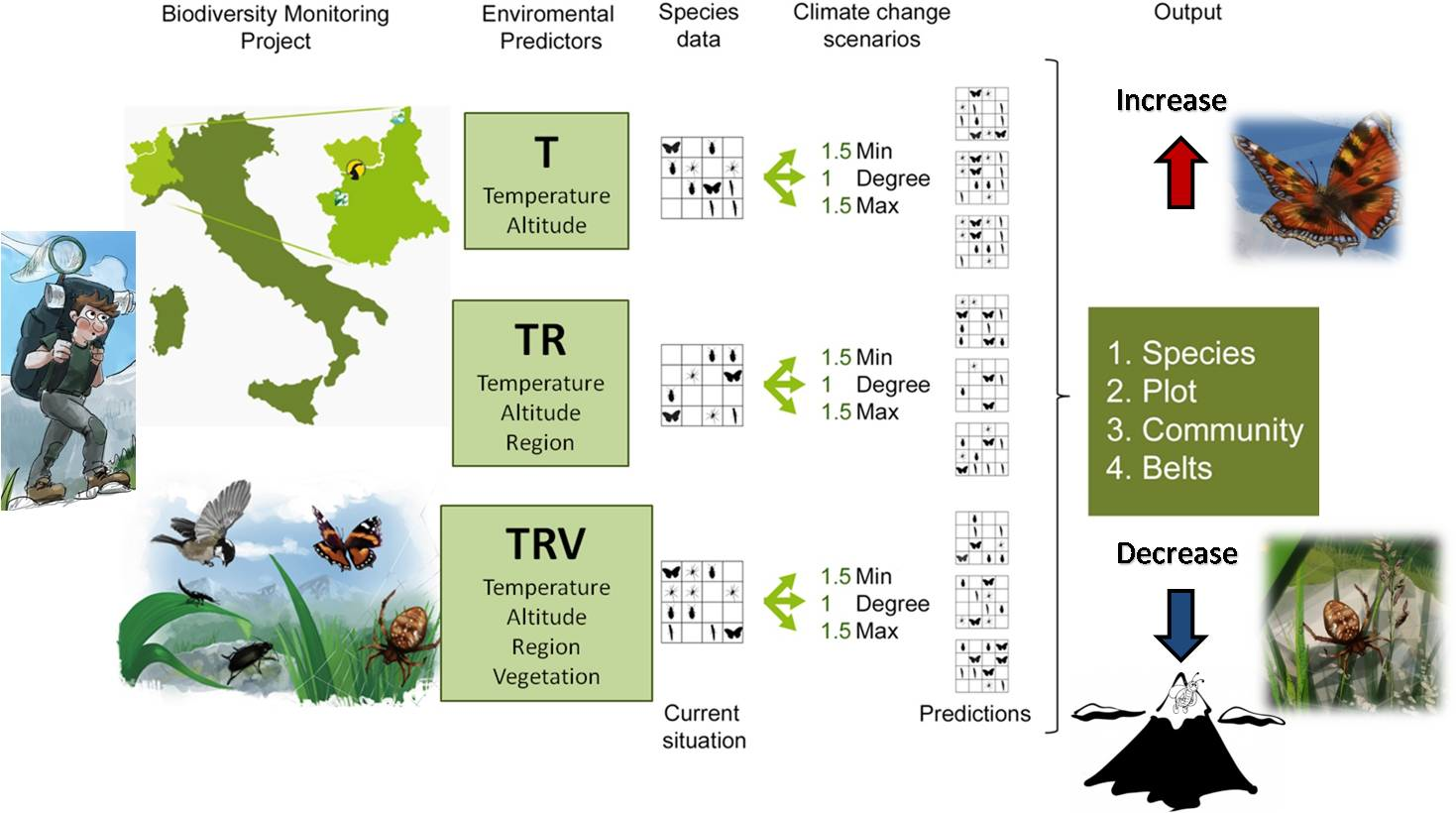
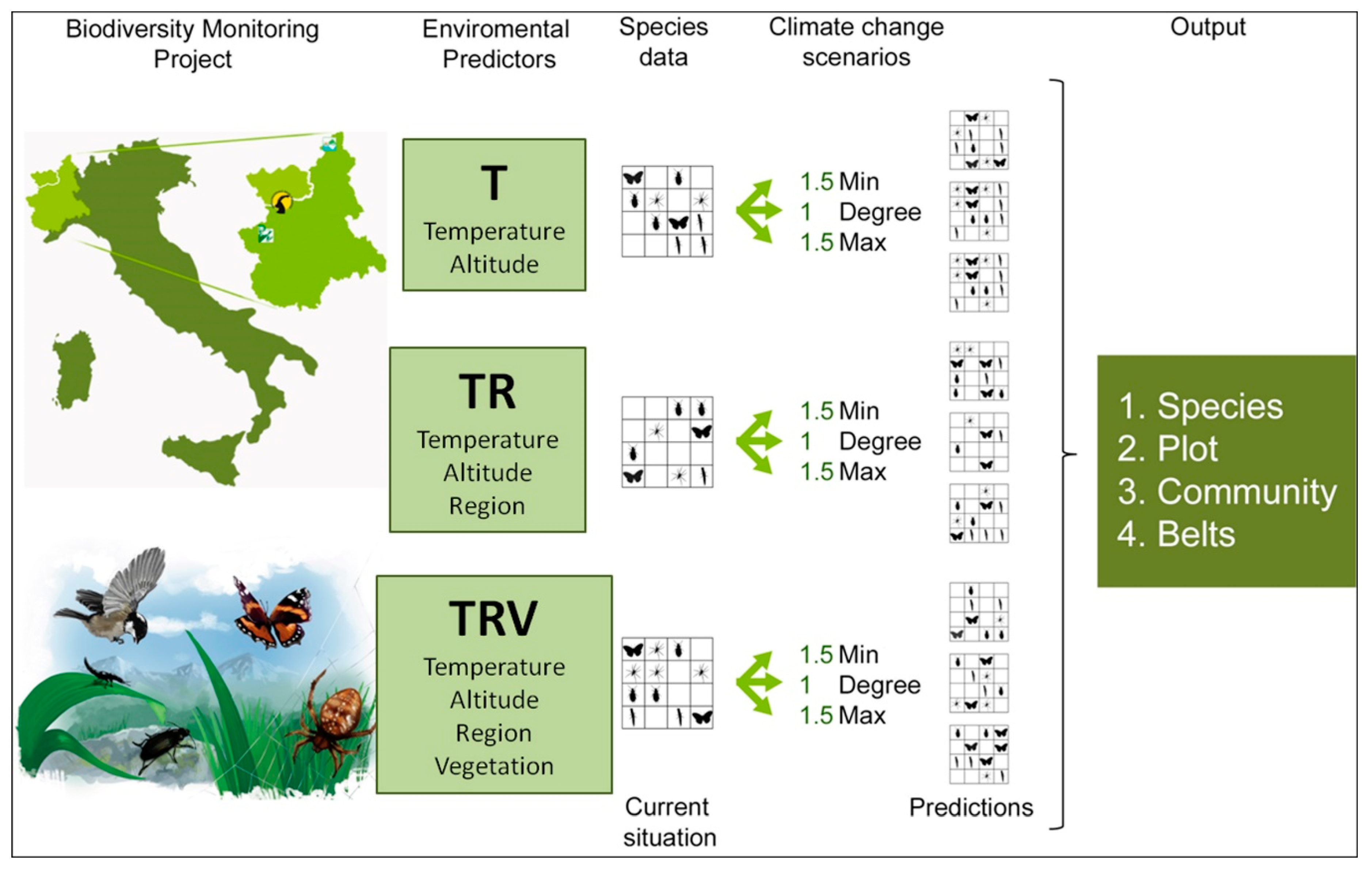
We combined the environmental predictors in different ways, obtaining three model classes with an increasing number of environmental constraints (Figure 1):
- Temperature (T), which considers only temperature-derived variables (seasonal mean, maximum, minimum temperature, and standard deviation, in °C) and altitude to model species distribution;
- Temperature+Region (TR), which considers temperature-derived variables, altitude, and geographical location;
- Temperature+Region+Vegetation Structure (TRV), which considers temperature-derived variables, altitude, geographical location, and vegetation cover.
To project species distributions for each model class (T, TR, TRV), we applied three different “what if” scenarios of temperature change:
- 1Degree (d), in which minimum, mean, and maximum temperature are all equally increased by 1 °C;
- 1.5Min (min), in which minimum temperature is increased by 1.5 °C, mean temperature by 1 °C, maximum temperature by 0.5 °C;
- 1.5Max (max), in which minimum temperature is increased by 0.5 °C, mean temperature by 1 °C, maximum temperature by 1.5 °C.
We based our choices on results from the analysis of temperature trends in the Alps, especially on [14] and [85], which reported a larger increase for minimum and maximum temperature respectively, and on [20] for future scenarios. Elevation-dependent warming is of relevance for most mountain regions [17], but the temperature increase can be taken as relatively homogeneous in the range of elevations considered here, even in the case of the Alpine belt [86]. “What-if” scenarios based on assuming a given temperature (and precipitation) change are a relatively recent way to look at climate change impacts (e.g., [87,88]). This approach is adopted here, in a simplified form, owing to the difficulty of regional climate models to properly represent future climatic changes in mountain areas of a limited extent [89].
We determined model accuracy by evaluating the area under the receiver operating characteristics curve (AUC), using the same dataset employed for training. This provided an optimistic measure of prediction success [90], which was anyway useful to assess warming effects on small datasets. Few species had an AUC < 0.6 (Table S2a–c; Figure S1) and we considered them to be stable under warming scenarios.
2.3. Analysis of Model Outputs
We transformed the model output into binary maps (presence/absence), using as threshold the minimum predicted value for the training sites, also termed “lowest presence threshold” [70,91].
This threshold identified as “species presence sites” all sites that are at least as suitable as those where the species is known to occur. After running the models for each individual species, thus allowing for different responses of different species, we calculated the α- and ß- diversity parameters to estimate changes from the current situation (defined as Maxent modelization before temperature increase scenarios), following the recommendations of [92].
2.3.1. Species Distribution
For each model class, we compared each warming scenario with the current distribution in terms of the number of occupied plots for each species.
We identified the species that significantly changed their distribution under warming (varying species), using a two-tailed binomial test. The number of successes was estimated from the number of occupied plots following the temperature increase, which was then compared to the number of plots currently occupied. To verify whether the three scenarios and the three model classes significantly differed in the number of varying species, we calculated the χ2 statistics on the contingency tables.
2.3.2. Species Richness
For each model class, we compared the distribution obtained in each warming scenario with the current distribution, in terms of species richness per plot. The differences were tested using the t-test for paired samples (significance level assessed after 999 randomizations, following [93]).
We quantified the changes in species richness per plot, for each model class and warming scenario, as:
where ES is the effect size, Sc is the current species richness, and Sp is the projected species richness. The increases and decreases of ES are symmetrical and range from −2 to +2 [94].
ES = (Sc − Sp)/(0.5 * (Sc + Sp))
To identify taxa that are more sensitive to the temperature increase, we analyzed the effect size as a function of the taxonomic group (considering as baseline the ensemble of all taxa). To this end, we used linear mixed-effects models with plot identity as a random effect.
We carried out an exploratory analysis using model classes, scenarios, and taxa and their interactions as explanatory variables. We selected the best model based on the Akaike’s Information Criterion corrected for small samples (AICc), computed with the “MuMIn” package [95]. Since the best model included no effects of warming scenarios, identifying instead a significant interaction of taxa and model class (Table S3), we then applied the linear mixed-effects models to each taxon separately, with the model class as an explanatory variable.
To understand how effect size changed as a function of elevation, we first graphically analyzed its variation along the altitudinal gradient and then focused on the differences between vegetation belts using again the linear-mixed effects models (with plot identity as a random effect).
Linear mixed-effects models have been implemented with the “lme4” package [96].
2.3.3. Community Composition
We represented changes in assemblage composition under warming scenarios by applying correspondence analysis (CA) to each taxon and model class. We focused on the first two CA-axes, whose explained variances were always significant (based on 999 randomizations obtained by changing species presence across plots while keeping prevalence constant). The cumulative explained variances ranged from 32.26 to 63.80 (Table S4a). The first axis was determined by altitude, minimum, and average daily temperature, while for the second axis we did not identify a clear pattern (Table S4b). To understand whether warming changed community composition as a whole and across vegetation belts, we applied the Wilcoxon Rank Sum Test on plot scores of current and projected distributions and compared the shift in plot scores between vegetation belts, using the Kruskal Wallis Test. Community homogenization under temperature increase was tested, comparing the distance from the distribution centroid for current and projected assemblages. Significance was assessed by the t-test for paired samples (using 999 randomizations [93]).
The variation in community composition of single plots under climate warming scenarios was quantified by the Jaccard Index and compared across model classes, scenarios, and taxa by the Friedman Test [97]. We also partitioned the overall dissimilarity in its turnover (βsim) and nestedness (βsne) components, calculated using the betapart package [98]. This allowed us to quantify whether communities exposed to temperature increase were characterized by the substitution of some species by others (turnover) or whether one of the two assemblages was a subset of the other (nestedness).
In the following, all values are represented as mean ± standard error; statistical analyses were performed using R 3. 5.2 [99].
3. Results
3.1. Species Distribution
The comparison between the results provided by each scenario and the corresponding baseline showed high variability in the species response to the temperature increase.
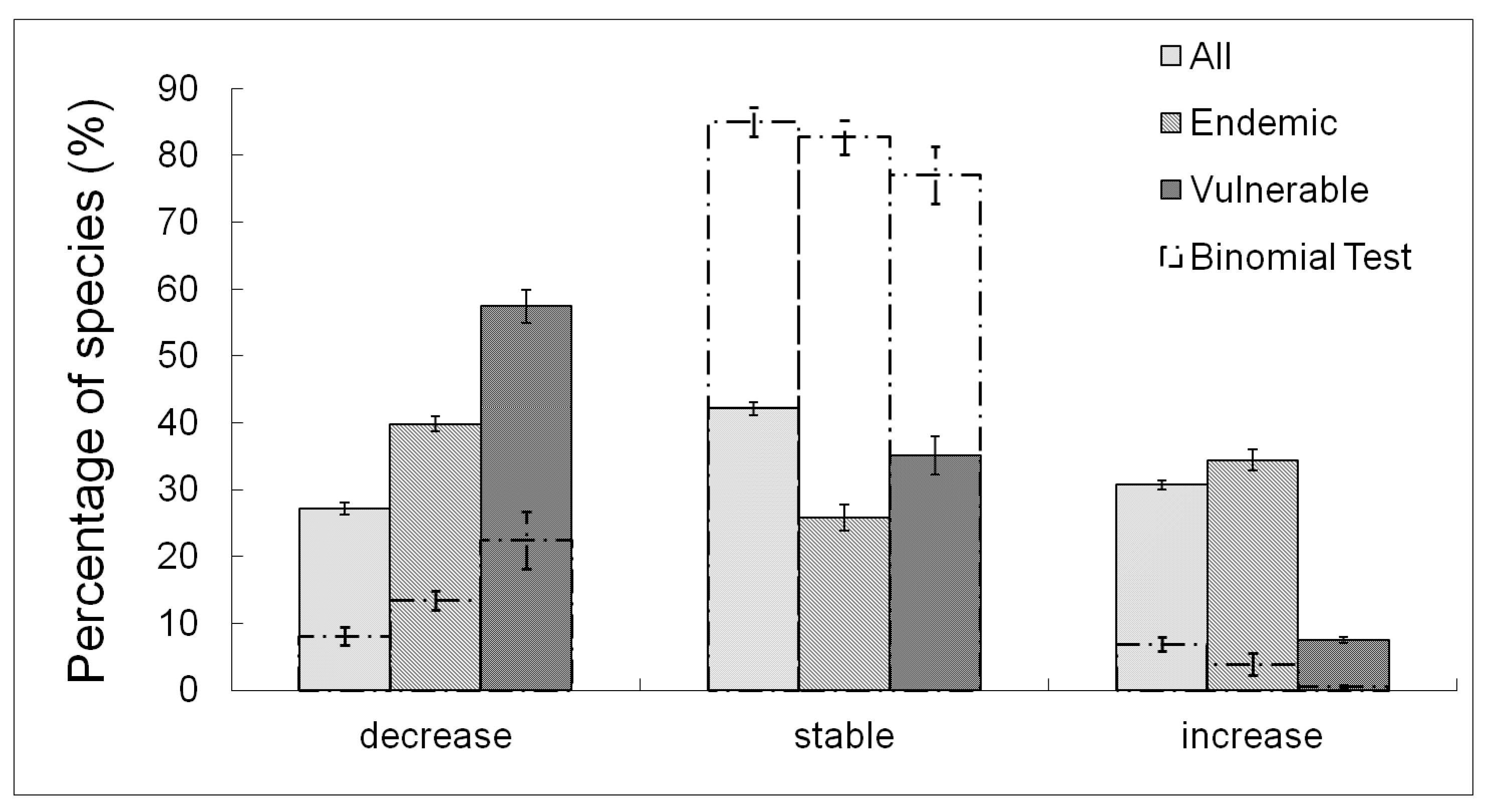
The majority of species showed no variation (42.1 ± 1.0%), some others displayed an increase (30.7 ± 0.7%), and others a decrease in the number of occupied plots (27.1 ± 0.9%). Considering only endemic and vulnerable species, the percentage of species with decreasing occupancy was higher (39.8 ± 1.1% for endemics; 57.4 ± 2.5% for vulnerable species) and in the case of the vulnerable species, the percentage of increasing species also became lower (7.5 ± 0.7%). Considering only varying species, both the endemic and the vulnerable species showed a higher percentage of decreasing occupancies and a lower percentage of increasing species, when compared to the whole set of species (Figure 2).
For the species that showed a variation, the amount of change was usually low (1st quartile = −4, median = 1, 3rd quartile = +4), even if the values ranged between −28 and +21 plots.
Comparing the three model classes, we found that the number of species with changing distributions was lower with a larger number of environmental constraints. Indeed, varying species in each scenario significantly differed between model classes (TRV = 25.7 ± 4.4, TR = 43.7 ± 4.4, T = 67.7 ± 8.4; 20.64 < χ2 < 27.82, p < 0.001).
Comparing the three scenarios, we observed a higher number of varying species in the Min scenario (Max = 37.3 ± 10.7, Min = 56.7 ± 14.6, D = 43.0 ± 11.3) in each model class, but the differences were significant only in the T model class (χ2 = 8.56, p = 0.02).
3.2. Species Richness
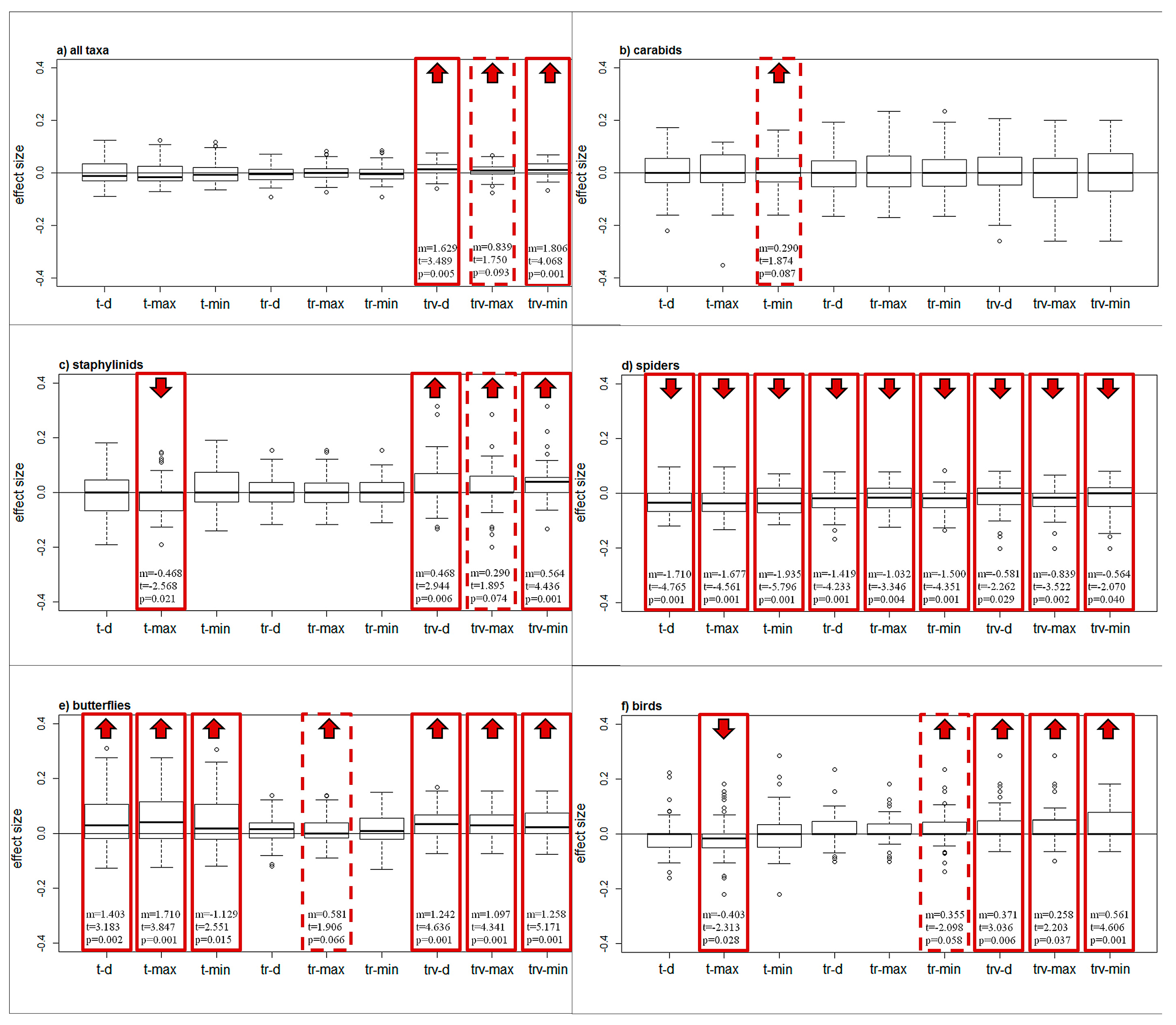
Changes in species richness showed considerable variations across taxonomic groups, warming scenarios, and vegetation belts, even if the amount of change was generally low, as exemplified by the effect size, ranging from −0.4 to 0.3 (Figure 3).
Butterflies displayed an increase in species richness per plot for almost all models and warming scenarios (Figure 3e); the impact of temperature increase is significantly stronger on this taxon than for all taxa pooled together (Table 1).
In the case of spiders, the results showed the opposite trend, with a decrease in species richness in all cases (Figure 3d) and significantly lower effect size than for all taxa pooled together (Table 1). Carabids showed no significant differences in any of the scenarios (Figure 3b). Staphylinids (Figure 3c) and birds (Figure 3f) showed slightly different results when considering different model classes.
The overall species richness showed a significant increase considering only the TRV model class.
For all taxa except carabids, we observed significant differences in the species richness changes predicted by the different model classes (Table 2). For butterflies, T models indicate an increase in species richness, which is less pronounced for TR and TRV models. For spiders, T models indicate a more pronounced decrease in species richness than TRV models. For all taxa pooled together, staphylinids and birds, TRV models indicate a significantly larger effect than T and TR models.
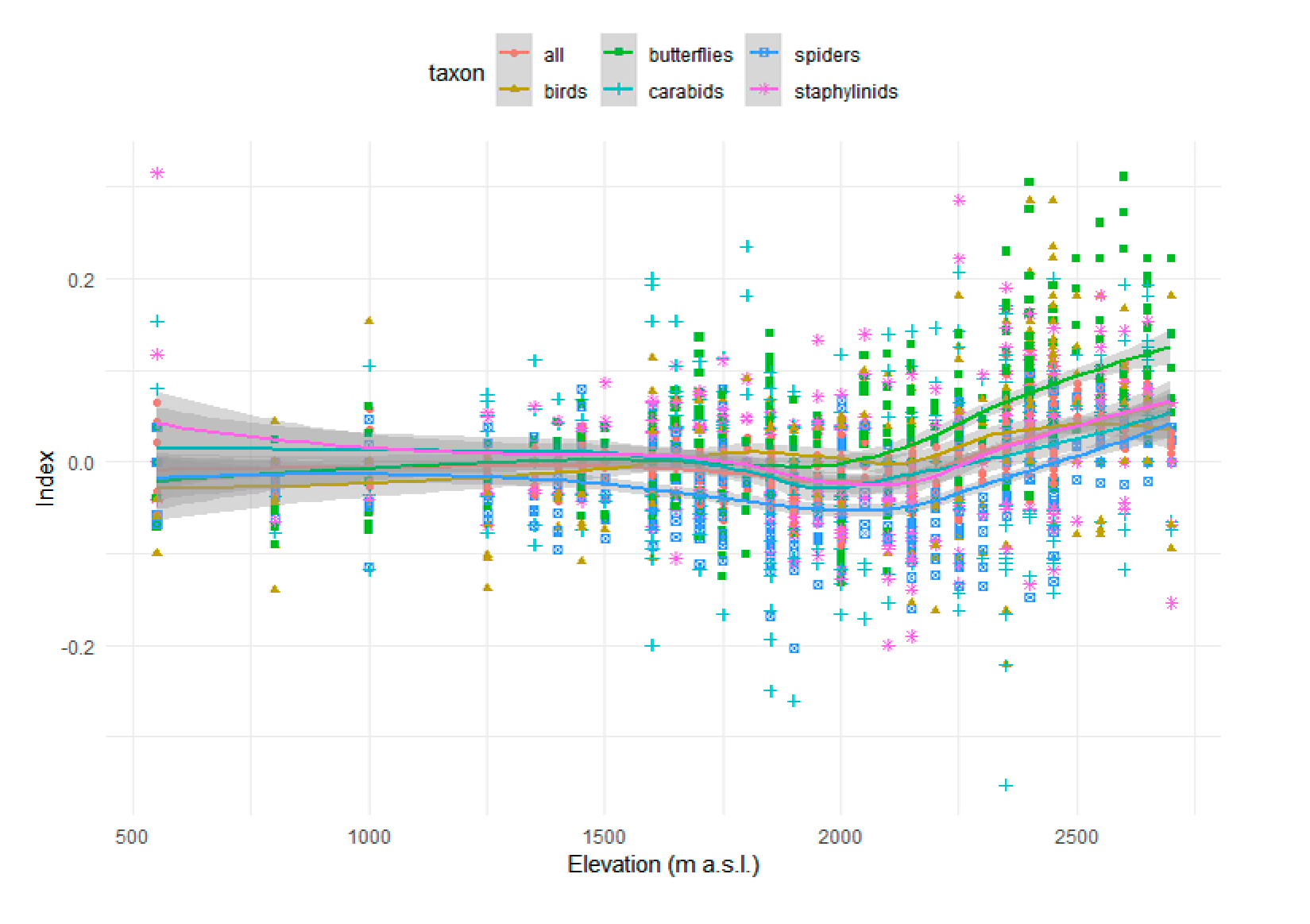
The analysis of changes in species richness along the altitudinal gradient indicated a more pronounced effect at higher altitude, in particular above 2000 m (Figure 4). In the Alpine belt, we observed a significant effect for all taxa pooled together, for butterflies, for birds and for spiders (Table 3). In the case of spiders, this implies that the decrease in species richness observed in the montane and the subalpine belt is less pronounced at higher altitudes (Figure 4; Table 3).
3.3. Community Composition
In almost all cases, warming scenarios determined significant changes in community composition along the first CA axis. The Wilcoxon test was applied to assess changes in plot scores from current to warmer conditions; it is significant in 53 over 54 cases, p < 0.01, the only exception are staphylinids in the TRV model class, max scenario. The pattern along the second axis is less coherent (Wilcoxon test with p < 0.01 in 35 cases over 54).
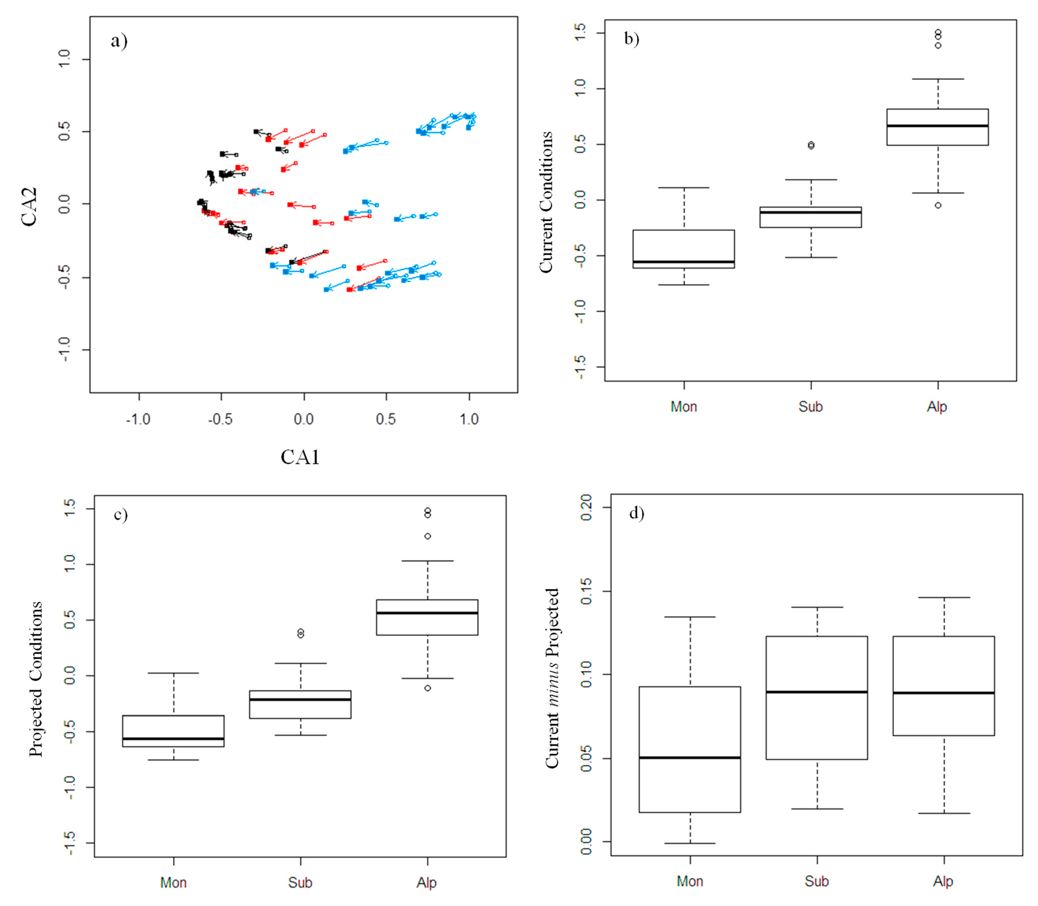
For both the current conditions and the warming scenarios, plot community composition significantly changed from the montane to the alpine belt (Figure 5a; current, KW Test, df = 2, all p < 0.0001, Figure 5b; projected, KW Test, df = 2, all p < 0.0001; Figure 5c).
Plot scores were significantly correlated in all cases (Spearman’s rank correlation; first axis, 0.978 < ρ < 0.998; second axis, 0.894 < ρ < 0.997), indicating that species composition changed gradually and coherently along the altitudinal gradient, retaining similar patterns of species dissimilarity.
Differences in the first axis between pairs of plots (current minus projected), if significant, showed that the amount of change in community composition was more pronounced for the montane belt compared to the others (Figure 5d). Interestingly, we observed significant differences for all taxa pooled together (for all model classes and scenarios), and in many cases also for carabids (T and TR, all scenarios), staphylinids (only T, Min and D scenarios), and butterflies (T, all scenarios; TR, Min and D scenarios; TRV, Max scenario), always showing the lowest values (around 0) for the montane belt.
As an estimate of community homogenization, we estimated the mean Euclidean distance from the distribution centroid for current conditions and for warming scenarios, showing always lower values in the warming case (which were also significant in 29 to 54 cases, p < 0.05).
The Jaccard Index values were close to zero for all model classes and scenarios. Considering all taxa pooled together, we observed significant differences across scenarios (p < 0.0001), with the lowest values in Max, and across model classes (p < 0.0001), with the highest values in T.
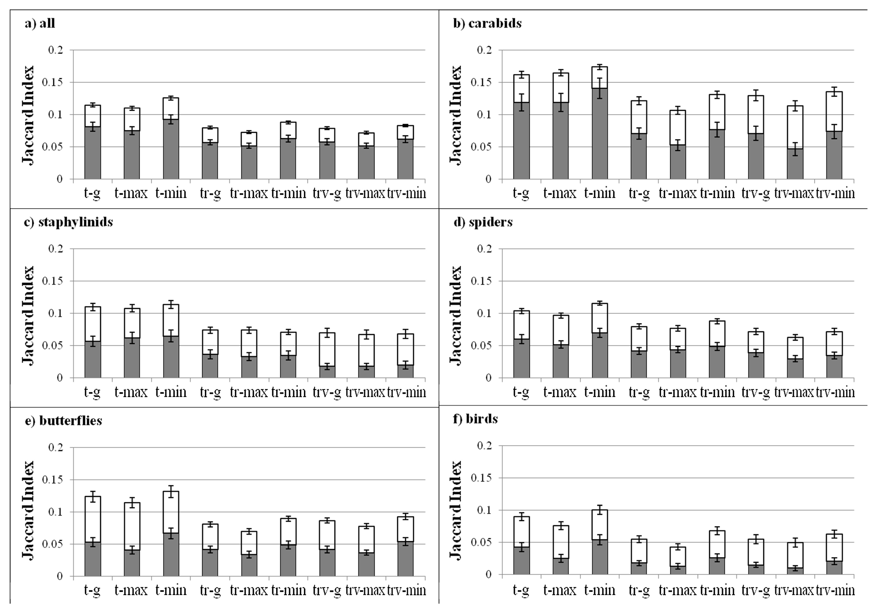
For all taxa pooled together (Figure 6a), the variation in community composition in the warming scenarios is dominated by turnover (βsim = 0.066 ± 0.005). The nestedness component is lower (βsne = 0.026 ± 0.002), indicating no clear pattern of species loss or gain. This global pattern has been observed also for carabids and spiders (Figure 6b,d), while in the case of butterflies and birds, differences are less pronounced and there is a tendency toward higher values of nestedness (Figure 6e,f). Staphylinids show no clear pattern (Figure 6c).
4. Discussion
Disentangling the role of temperature increase in shaping biodiversity patterns, especially in mountain ecosystems, is a fundamental challenge of conservation biology [2,3,8]. Species respond at individual level [1,2] and there is a current knowledge gap for many taxonomic groups [31,32,33,49]. Projections of potential future species distributions along elevational gradients need high-resolution spatial data [83,100]. In our work, the Maxent approach allowed to analyze data collected at a fine spatial scale (plots with 100 m radius) and to take into account the response of rare and localized species. Reliable projections should also consider that ecotypes from different geographical origins can have different responses to the same climatic variations (e.g., [101]). Our approach reduced this bias in two ways. First, we used the same set of plots to derive the empirical relationships between species and climatic/environmental variables and to project future potential distributions. Second, the limited geographic extent (northwestern Italian Alps) of the sampled plots assures that different populations of the same species will respond coherently.
In general, our simulations indicated that even for a moderate temperature increase, species richness and community composition can display subtle but significant alterations. Since different studies suggested different roles of minimum and maximum temperature increase [14,85], we simulated three scenarios having different relative importance of the minimum and maximum daily temperature rise. We also adopted three different empirical biodiversity model classes, characterized by the presence of temperature alone or of other environmental variables (vegetation and geographical location) in addition to temperature. Differences between scenarios were not as marked as those emerging from the different model classes.
We detected a high variability in the response of the different species, depending on the position and breadth of the climatic niche and the species range. The majority of modeled species did not show much response to the temperature increase. On the other hand, high-altitude species were the most affected, consistently with the fact that habitat specialists are negatively influenced by environmental change (e.g., [7]). The probability of extinction under climate change reflects the species ability to shift with suitable habitats; a scarce ability to withstand climate change impacts could depend also on a reduced niche breadth [7,102,103].
In our analysis, endemic species appeared as less affected than vulnerable ones. In the altitudinal gradient explored here, the spatial distribution of endemic species is spread over the whole altitudinal and temperature range, owing to the presence of species that are characteristic of the montane belt. Our results indicate that many of the endemic species studied here are not restricted to high altitudes and can shift their occupancy area along the altitudinal gradient. These results are not in disagreement with the general vulnerability of endemic species to climate change (e.g., [7,104]): thanks to the small scale of the analysis, our study indicates how local altitudinal gradients can offer a possibility of survival for otherwise declining species.
Significant differences between taxonomic groups were also observed.
Carabids did not show any relationship with temperature [52] and, as a consequence, they did not display any significant change in species richness under temperature increase scenarios. On the other hand, they displayed the highest “temporal dissimilarity” in community composition (even if always low, with an overall Jaccard index < 0.15). This behavior was mainly determined by turnover, i.e., by the substitution of groups of species under climate warming.
In the case of staphylinids, the pattern of change was also not marked: few significant differences were observed, and they were not coherent across model classes and scenarios, hampering the possibility of drawing general considerations.
Butterflies are heliothermic and can be considered climatically sensitive [33,105]. In our analysis, for many species the distribution was mainly determined by temperature. This taxon displayed the highest increase in species richness under temperature increase. This pattern is exacerbated by the model classes using temperature only as a constraint, and it is particularly strong in the alpine belt. These results indicate that butterflies can respond quickly to warming, determining new species assemblages, in particular at high altitudes and that the vegetation structure has the potential to buffer this response. Similar results were found analyzing observed temporal changes in butterfly distribution and community composition [106,107], also during a short time frame [108] and in the same mountain ranges considered here [53].
On the opposite side, spiders strongly suffered in temperature increase scenarios, showing a decrease in species richness. In our monitoring program, spiders were highly localized and many species were present only in a small number of plots. Therefore, variations of microclimatic conditions can effectively reduce their areas of occurrence, determining a general decrease in species richness. Models using only temperature provide the most marked changes, indicating again that the vegetation structure can buffer the effects of warming. For spiders, the highest decrease in species richness was observed in the montane belt. Our results suggest that the montane belt will become too warm for many species. Indeed, spider species are usually influenced by the small-scale vegetation structure and are adapted to the local environmental conditions [109,110]. This leads to a high level of turnover along altitudinal gradients and consequently to assemblages that are sensitive to small changes in local climatic conditions, as observed here.
Birds display a significant increase in species richness for many of the tested models and scenarios and a general positive effect of warming. Temporal analysis of bird and butterfly communities showed that both taxa respond to warming, with a faster response of butterflies [106]. For birds, changes in community composition were dominated by the nestedness component, indicating that species losses and gains represent the principal pattern of change.
Considering “temporal” dissimilarity as a whole, we observed significant changes for all cases (model classes, scenarios, taxa). Plot assemblage composition coherently changed in warming scenarios, showing a tendency to homogenization as observed in other studies [111,112,113].
As in other studies focused on plants [11], our warming scenarios indicated an upward shift from the lower to the higher belts, implying an increase in species richness at the highest altitude. Alpine meadows had a high probability of experiencing the largest modifications in community composition, as we coherently observed for almost all taxa. Such changes in richness and composition, if effectively realized, will probably be detrimental to biodiversity: the colonization of the alpine belt by species from lower altitudes could increase competition, with negative effects for localized and specialized taxa [13,114,115]. Consequently, the increase in species richness could be transitory, followed by a decline of strictly alpine species stressed by the growing competition and on the verge of going beyond their tolerance breadth [24,116].
The montane belt, on the opposite, is the lower limit of the altitudinal gradient considered here and we cannot account for the colonization of species coming from still lower elevations. We classified plots along the vegetation belts considering both altitude and potential vegetation [65,66]: consequently, some montane plots display temperature values that are lower than for subalpine ones, allowing for a partial increase in species richness under climate warming. In any case, the montane belt community composition was the most stable, showing lower dissimilarity than the upper two belts.
Among the different warming scenarios, the one with a larger increase of minimum temperature displayed the largest number of varying species, indicating that the minimum daily temperature can be an important limiting factor for species distribution [65,66]. Considering that the minimum temperature has increased at a faster rate than the maximum temperature during the latter half of the 20th century [117], variations in biodiversity patterns larger than the ones simulated here could occur.
Even if uncertainty is the rule in species distribution models [40,45], projections are useful to explore biodiversity patterns, identifying specific areas or groups of species that should be monitored. In this regard, the different responses displayed by different taxa confirm the importance of using a multi-taxa approach to estimate climate change effects on animal biodiversity. It is important to include taxa with potentially opposite responses to climate warming, such as butterflies and spiders. Targeted long-term field data are then essential to revisit and fine-tune estimates of biodiversity responses, comparing them with real changes in species responses, and adopting timely conservation strategies [118].
Even if the alpine belt displayed the highest projected change in species richness, monitoring focused only on high altitudes could miss some of the important changes along the altitude gradient. The high level of turnover due to species shifts from the montane and to the alpine belts could happen also in the subalpine belt, and the montane belt can be influenced by the arrival of species from the surrounding lowlands.
In conclusion, our analysis suggested that moderate warming has the potential to change biodiversity patterns in mountain ecosystems, with significant differences between taxa and along the altitudinal gradient. Such changes could determine new ecological relationships, which could in turn influence ecosystem processes in an unpredictable way.
Supplementary Materials
The following material is available online at https://0-www-mdpi-com.brum.beds.ac.uk/1424-2818/12/6/210/s1. Table S1. Plot characteristics. Table S2a. Species used in the modeling approach. Table S2b. AUC thresholds. Table S2c. Species richness correlations. Figure S1. AUC values. Table S3. Explorative model selection. Table S4a. Explained variances of CA axes. Table S4b. Correlation of CA axes with environmental variables.
Author Contributions
Conceptualization, R.V., A.P. and C.C.; methodology, R.V., A.P. and C.C.; formal analysis, R.V. and C.C.; investigation, R.V., R.B. and C.C.; data curation, R.V., R.B. and C.C.; writing—original draft preparation, R.V., R.B., C.C. and A.P.; writing—review and editing, R.V., R.B., C.C. and A.P.; visualization, R.V., R.B., C.C. and A.P.; supervision, R.V. and A.P.; project administration, R.V. and A.P.; funding acquisition, R.V., R.B. and A.P. All authors have read and agreed to the published version of the manuscript.
Funding
This work was partially funded by the Project of Interest “NextData” of the Italian Ministry of Education, University and Research. The project leading to this research was coordinated by Gran Paradiso National Park and partially funded through the “Monitoraggio della biodiversità in ambiente alpino” grant (Progetti di Sistema ex cap.1551), provided by the Italian Ministry of the Environment (Ministero dell’Ambiente e della Tutela del Territorio e del Mare). This research also received funding from the European Union’s Horizon 2020 Research and Innovation Programme under grant agreement no. 641762 “Improving Future Ecosystem Benefits through Earth Observations” (Ecopotential).
Acknowledgments
We are grateful to the Park Directors, Laura Castagneri, Michele Ottino and Ivano De Negri for logistic support and data availability. We thank Bruno Bassano and Giuseppe Bogliani for their support and for the coordination of the field activities. We are grateful to all Park Wardens, collaborators and students for their essential help during the field work. We thank the taxonomists Gianni Allegro (Coleoptera Carabidae), Sara de Angelis (Araneae), Alessandro Fantoni (Araneae), Paolo Palmi (Lepidoptera Papilionoidea and Hesperiioidea), Aurelio Perrone (Aves) and Adriano Zanetti (Coleoptera Staphylinidae) for the help with fieldwork and the identification of the huge amount of collected samples.
Conflicts of Interest
The authors declare no conflict of interest. The funders had no role in the design of the study; in the collection, analyses, or interpretation of data; in the writing of the manuscript, or in the decision to publish the results.
References
- Walther, G.R. Community and ecosystem responses to recent climate change. Philos. Trans. R. Soc. B 2010, 365, 2019–2024. [Google Scholar] [CrossRef]
- Bellard, C.; Bertelsmeier, C.; Leadley, P.; Thuiller, W.; Courchamp, F. Impacts of climate change on the future of biodiversity. Ecol. Lett. 2012, 15, 365–377. [Google Scholar] [CrossRef] [PubMed] [Green Version]
- Settele, J.; Scholes, R.; Betts, R.A.; Bunn, S.; Leadley, P.; Nepstad, D.; Overpeck, J.T.; Taboada, M.A.; Fischlin, A.; Moreno, J.M.; et al. Terrestrial and inland water systems. In Climate Change 2014: Impacts, Adaptation, and Vulnerability. Part A: Global and Sectoral Aspects. Contribution of Working Group II to the Fifth Assessment Report of the Intergovernmental Panel on Climate Change; Field, C.B., Barros, V.R., Dokken, D.J., Mach, J.K., Mastrandrea, M.D., Bilir, T.E., Chatterjee, M., Ebi, K.L., Estrada, Y.O., Genova, R.C., et al., Eds.; Cambridge University Press: Cambridge, UK, 2014; pp. 271–359. [Google Scholar]
- Kujala, H.; Burgman, M.A.; Moilanen, A. Treatment of uncertainty in conservation under climate change. Conserv. Lett. 2013, 6, 73–85. [Google Scholar] [CrossRef] [Green Version]
- Reside, A.E.; Butt, N.; Adams, V.M. Adapting systematic conservation planning for climate change. Biodivers. Conserv. 2018, 27, 1–29. [Google Scholar] [CrossRef]
- Lloret, F. Trade-offs in high mountain conservation. In High Mountain Conservation in a Changing World; Catalan, J., Ninot, J., Aniz, M., Eds.; Advances in Global Change Research, 62; Springer: Berlin, Germany, 2017; pp. 37–59. [Google Scholar]
- Dirnböck, T.; Essel, F.; Rabitsch, W. Disproportional risk for habitat loss of high-altitude endemic species under climate change. Glob. Chang. Biol. 2011, 17, 990–996. [Google Scholar] [CrossRef]
- Huber, U.; Reasoner, M.; Bugmann, H. Global Change and Mountain Regions: An Overview of Current Knowledge; Advances Global Change Research; Springer: Berlin, Germany, 2005. [Google Scholar]
- Diaz, H.F.; Grosejeanan, M.; Graumlich, L. Climate variability and change in high elevation regions: Past, present and future. Clim. Chang. 2003, 59, 1–4. [Google Scholar] [CrossRef]
- Nogués-Bravo, D.; Araújo, M.; Erread, M.P.; Martínez-Rica, J.P. Exposure of global mountain systems to climate warming during the 21st Century. Glob. Environ. Chang. 2007, 17, 420–428. [Google Scholar] [CrossRef]
- Grabherr, G.; Gottfried, M.; Pauli, H. Global change effects on alpine plant diversity. In Biodiversity Hotspots. Distribution and Protection of Conservation Priority Areas; Zachos, F.E., Habel, J.C., Eds.; Springer: Berlin, Germany, 2011; pp. 529–536. [Google Scholar]
- Schmitt, T. Biogeographical and evolutionary importance of the European high mountain systems. Front. Zool. 2009, 6, 1–9. [Google Scholar] [CrossRef] [Green Version]
- Pauli, H.; Gottfried, M.; Reiter, K.; Klettner, C.; Grabherr, G. Signals of range expansions and contractions of vascular plants in the high Alps: Observations (1994–2004) at the GLORIA master site Schrankogel, Tyrol, Austria. Glob. Chang. Biol. 2007, 13, 147–156. [Google Scholar] [CrossRef]
- Beniston, M. Mountain weather and climate: A general overview and a focus on climatic change in the Alps. Hydrobiologia 2006, 562, 3–16. [Google Scholar] [CrossRef] [Green Version]
- Calmanti, S.; Motta, L.; Turco, M.; Provenzale, A. Impact of climate variability on Alpine glaciers in northwestern Italy. Int. J. Climatol. 2007, 27, 2041–2053. [Google Scholar] [CrossRef]
- Keiler, M.; Knight, J.; Harrison, S. Climate change and geomorphological hazards in the eastern European Alps. Philos. Trans. R. Soc. A 2010, 368, 2461–2479. [Google Scholar] [CrossRef] [PubMed] [Green Version]
- Pepin, N.; Bradley, R.S.; Diaz, H.F.; Baraer, M.; Cáceres, B.; Forsythe, N.; Fowler, H.J.; Greenwood, G.; Ziaur Rahman Hashmi, M.; Liu, X.D.; et al. Elevation-dependent warming in mountain regions of the world. Nat. Clim. Chang. 2015, 5, 424–430. [Google Scholar]
- Intergovernmental Panel on Climate Change (IPCC). Special Report on the Ocean and Cryosphere in a Changing Climate. Available online: https://www.ipcc.ch/srocc/ (accessed on 25 March 2020).
- Poussin, C.; Guigoz, Y.; Palazzi, E.; Terzago, S.; Chatenoux, B.; Giuliani, G. Snow cover evolution in the Gran Paradiso National Park, Italian Alps, using the Earth Observation data cube. Data 2019, 4, 138. [Google Scholar] [CrossRef] [Green Version]
- Gobiet, A.; Kotlarski, S.; Beniston, M.; Heinrich, G.; Rajczak, J.; Stoffel, M. 21st century climate change in the European Alps—A review. Sci. Total Environ. 2014, 493, 1138–1151. [Google Scholar] [CrossRef] [PubMed]
- Pachauri, R.K.; Allen, M.R.; Barros, V.R.; Broome, J.; Cramer, W.; Christ, R.; Church, J.A.; Clarke, L.; Dahe, Q.; Dasgupta, P.; et al. Climate Change 2014: Synthesis Report. Contribution of Working Groups I, II and III to the Fifth Assessment Report of the Intergovernmental Panel on Climate Change; Pachauri, R., Meyer, L., Eds.; IPCC: Geneva, Switzerland, 2014. [Google Scholar]
- Payne, D.; Spehn, E.M.; Snethlage, M.; Fischer, M. Opportunities for research on mountain biodiversity under global change. Curr. Opin. Environ. Sustain. 2017, 29, 40–47. [Google Scholar] [CrossRef]
- Theurillat, J.P.; Guisan, A. Potential impact of climate change on vegetation in the European Alps: A review. Clim. Chang. 2001, 50, 77–109. [Google Scholar] [CrossRef]
- Lesica, P.; McCune, B. Decline of arctic-alpine plants at the southern margin of their range following a decade of climatic warming. J. Veg. Sci. 2004, 15, 679–690. [Google Scholar] [CrossRef]
- Winkler, D.; Lubetkin, K.C.; Carrell, A.A.; Jabis, M.D.; Yang, Y.; Kueppers, L.M. Responses of alpine plant communities to climate warming. In Ecosystem Consequences of Soil Warming; Mohan, J.E., Ed.; Academic Press: London, UK, 2019; pp. 297–346. [Google Scholar]
- Battisti, A.; Stastny, M.; Netherer, S.; Robinet, C.; Schopf, A.; Roques, A.; Larsson, S. Expansion of geographic range in the processionary moth caused by increased winter temperatures. Ecol. Appl. 2005, 15, 2084–2096. [Google Scholar] [CrossRef]
- Wilson, R.J.; Gutiérrez, D.; Gutiérrez, D.M.; Agudo, R.; Monserrat, V.J. Changes to the elevation limits and extent of species ranges associated with climate change. Ecol. Lett. 2005, 8, 1138–1146. [Google Scholar] [CrossRef]
- Gobbi, M.; Fontaneto, D.; de Bernardi, F. Influence of climate changes on animal communities in space and time: The case of spider assemblages along an alpine glacier foreland. Glob. Chang. Biol. 2006, 12, 1985–1992. [Google Scholar] [CrossRef]
- Buntgen, U.; Greuter, L.; Bollman, K.; Jenny, H.; Liebhold, A.; Galvan, J.D.; Stenseth, N.C.; Andrew, C.; Mysterud, A. Elevational range shifts in four mountain ungulate species from the Swiss Alps. Ecosphere 2017, 8, e01761. [Google Scholar] [CrossRef]
- Menéndez, R.; Megías, A.G.; Hill, J.K.; Braschler, B.; Willis, S.G.; Collingham, Y.; Fox, R.; Roy, D.B.; Thomas, C.D. Species richness changes lag behind climate change. Proc. R. Soc. B 2006, 273, 1465–1470. [Google Scholar] [CrossRef] [PubMed] [Green Version]
- Cardoso, P.; Erwin, T.L.; Borges, P.A.V.; New, T.R. The seven impediments in invertebrate conservation and how to overcome them. Biol. Conserv. 2011, 144, 2647–2655. [Google Scholar] [CrossRef] [Green Version]
- Nooten, S.S.; Andrew, N.R. Transplant experiments—A powerful method to study climate change impacts. In Invertebrates and Global Climate Change; Johnson, S., Jones, H., Eds.; Wiley-Blackwell: Oxford, UK, 2017; pp. 46–67. [Google Scholar]
- Palmer, G.; Hill, J.K. Using historical data for studying range changes. In Invertebrates and Global Climate Change; Johnson, S., Jones, H., Eds.; Wiley-Blackwell: Oxford, UK, 2017; pp. 9–29. [Google Scholar]
- Ferrier, S.; Guisan, A. Spatial modelling of biodiversity at the community level. J. Appl. Ecol. 2006, 43, 393–404. [Google Scholar] [CrossRef]
- Margules, C.R.; Pressey, L.R. Systematic conservation planning. Nature 2000, 405, 243–253. [Google Scholar] [CrossRef] [PubMed]
- Araújo, M.B.; Alagador, D.; Cabeza, M.; Nogués-Bravo, D.; Thuiller, W. Climate change threatens European conservation areas. Ecol. Lett. 2012, 14, 484–492. [Google Scholar] [CrossRef] [Green Version]
- Dunlop, M. Biodiversity: Strategy conservation. Nat. Clim. Chang. 2013, 3, 1019–1020. [Google Scholar] [CrossRef]
- Heller, N.E.; Zavaleta, E.S. Biodiversity management in the face of climate change: A review of 22 years of recommendations. Biol. Conserv. 2009, 142, 14–32. [Google Scholar] [CrossRef]
- Catalan, J.; Ninot, J.; Aniz, M. The High Mountain Conservation in a Changing World; Catalan, J., Ninot, J., Aniz, M., Eds.; Advances in Global Change Research, 62; Springer: Berlin, Germany, 2017; pp. 3–36. [Google Scholar]
- Elith, J.; Leathwick, J.R. Species distribution models: Ecological explanation and prediction across space and time. Annu. Rev. Ecol. Evol. Syst. 2009, 40, 677–697. [Google Scholar] [CrossRef]
- Guisan, A.; Thuiller, W. Predicting species distribution: Offering more than simple habitat models. Ecol. Lett. 2005, 8, 993–1009. [Google Scholar] [CrossRef]
- Guisan, A.; Tingley, R.; Baumgartner, J.B.; Naujokaitis-Lewis, I.; Sutcliffe, P.R.; Tulloch, A.I.T.; Regan, T.J.; Brotons, L.; McDonald-Madden, E.; Mantyka-Pringle, C.; et al. Predicting species distributions for conservation decisions. Ecol. Lett. 2013, 16, 1424–1435. [Google Scholar] [CrossRef] [PubMed]
- Guisan, A.; Thuiller, W.; Zimmermann, N.E. Habitat Suitability and Distribution Models—With Applications in R; Cambridge University Press: Cambridge, UK, 2017. [Google Scholar]
- Wiens, J.A.; Stralberg, D.; Jongsomjit, D.; Howell, C.A.; Snyder, M.A. Niches, models, and climate change: Assessing the assumptions and uncertainties. Proc. Natl. Acad. Sci. USA 2009, 106, 19729–19736. [Google Scholar] [CrossRef] [Green Version]
- Lavergne, S.; Mouquet, N.; Thuiller, W.; Ronce, O. Biodiversity and climate change: Integrating evolutionary and ecological responses of species and communities. Annu. Rev. Ecol. Evol. Syst. 2010, 41, 321–350. [Google Scholar] [CrossRef] [Green Version]
- Urban, M.C.; Bocedi, G.; Hendry, A.P.; Mihoub, J.B.; Pe’er, G.; Singer, A.; Bridle, J.R.; Crozier, L.G.; De Meester, L.; Godsoe, W.; et al. Improving the forecast for biodiversity under climate change. Science 2016, 353, aad8466. [Google Scholar] [CrossRef] [Green Version]
- Cotto, O.; Wessely, J.; Georges, D.; Klonner, G.; Schmid, M.; Dullinger, S.; Thuiller, W.; Guillaume, F. A dynamic eco-evolutionary model predicts slow response of alpine plants to climate warming. Nat. Commun. 2017, 8, 15399. [Google Scholar] [CrossRef] [PubMed] [Green Version]
- Dawson, T.P.; Jackson, S.T.; House, J.I.; Prentice, I.C.; Mace, G.M. Beyond predictions: Biodiversity conservation in a changing climate. Science 2011, 332, 53–58. [Google Scholar] [CrossRef] [PubMed] [Green Version]
- Arribas, P.; Abellán, P.; Velasco, J.; Millán, A.; Sánchez-Fernández, D. Conservation of insects in the face of global climate change. In Invertebrates and Global Climate Change; Johnson, S., Jones, H., Eds.; Wiley-Blackwell: Oxford, UK, 2017; pp. 349–367. [Google Scholar]
- Scherrer, D.; Massy, S.; Meier, S.; Vittoz, P.; Guisan, A. Assessing and predicting shifts in mountain forest composition across 25years of climate change. Divers. Distrib. 2017, 23, 517–528. [Google Scholar] [CrossRef] [Green Version]
- Khalyani, A.H.; Gould, W.A.; Falkowski, M.J.; Muscarella, R.; Uriarte, M.; Yousef, F. Climate change increases potential plant species richness on Puerto Rican uplands. Clim. Chang. 2019, 156, 15–30. [Google Scholar] [CrossRef]
- Viterbi, R.; Cerrato, C.; Bassano, B.; Bionda, R.; von Hardenberg, A.; Provenzale, A.; Bogliani, G. Patterns of biodiversity in the northwestern Italian Alps: A multi-taxa approach. Com. Ecol. 2013, 14, 18–30. [Google Scholar] [CrossRef]
- Cerrato, C.; Rocchia, E.; Brunetti, M.; Bionda, R.; Bassano, B.; Provenzale, A.; Bonelli, S.; Viterbi, R. Butterfly distribution along altitudinal gradients: Temporal changes over a short time period. Nat. Conserv. 2019, 34, 91–118. [Google Scholar] [CrossRef] [Green Version]
- Engler, R.; Randin, C.F.; Thuiller, W.; Dullinger, S.; Zimmermann, N.E.; Araújo, M.B.; Pearman, P.B.; le Lay, G.; Piedallu, C.; Albert, C.H.; et al. 21st century climate change threatens mountain flora unequally across Europe. Glob. Chang. Biol. 2011, 17, 2330–2341. [Google Scholar] [CrossRef]
- Thuiller, W.; Pollock, L.J.; Gueguen, M.; Münkemüller, T. From species distributions to meta-communities. Ecol. Lett. 2015, 18, 1321–1328. [Google Scholar] [CrossRef] [PubMed] [Green Version]
- Mouquet, N.; Lagadeuc, Y.; Devictor, V.; Doyen, L.; Duputié, A.; Eveillard, D.; Faure, D.; Garnier, E.; Gimenez, O.; Huneman, P.; et al. Review: Predictive ecology in a changing world. J. Appl. Ecol. 2015, 52, 1293–1310. [Google Scholar] [CrossRef]
- Perrigo, A.; Hoorn, C.; Antonelli, A. Why mountains matter for biodiversity. J Biogeogr. 2020, 47, 315–325. [Google Scholar] [CrossRef] [Green Version]
- Thuiller, W.; Münkemüller, T.; Lavergne, S.; Mouillot, D.; Mouquet, N.; Schiffers, K.; Gravel, D. A road map for integrating eco-evolutionary processes into biodiversity models. Ecol. Lett. 2013, 16, 94–105. [Google Scholar] [CrossRef] [Green Version]
- Boulangeat, I.; Georges, D.; Dentant, C.; Bonet, R.; Van Es, J.; Abdulhak, S.; Zimmermann, N.E.; Thuiller, W. Anticipating the spatio-temporal response of plant diversity and vegetation structure to climate and land use change in a protected area. Ecography 2014, 37, 1230–1239. [Google Scholar] [CrossRef]
- Chen, I.-C.; Hill, J.K.; Ohlemüller, R.; Roy, D.B.; Thomas, C.D. Rapid range shifts of species associated with high levels of climate warming. Science 2011, 333, 1024–1026. [Google Scholar] [CrossRef]
- McGeoch, M.A. The selection, testing and application of terrestrial insects as biondicators. Biol. Rev. 1998, 73, 181–201. [Google Scholar] [CrossRef]
- Kati, V.; Devillers, P.; Dufrêne, M.; Legakis, A.; Vokou, D.; Lebrun, P. Testing the value of six taxonomic groups as biodiversity indicators at a local scale. Conserv. Biol. 2004, 18, 667–675. [Google Scholar] [CrossRef]
- Sauberer, N.; Zulka, P.K.; Abensperg-Traun, M.; Berg, H.; Bieringer, G.; Milasowszky, N.; Moser, D.; Plutzar, C.; Pollheimer, M.; Storch, C.; et al. Surrogate taxa for biodiversity in agricultural landscapes of eastern Austria. Biol. Conserv. 2004, 117, 181–190. [Google Scholar] [CrossRef]
- Hodkinson, I.D.; Jackson, J.K. Terrestrial and aquatic invertebrates as bioindicators for environmental monitoring, with particular reference to mountain ecosystems. Environ. Manag. 2005, 35, 649–666. [Google Scholar] [CrossRef] [PubMed]
- Körner, C.; Paulsen, J.; Spehn, E. A definition of mountains and their bioclimatic belts for gr global comparisons of biodiversity data. Alp. Bot. 2011, 121, 73–78. [Google Scholar] [CrossRef] [Green Version]
- Beniston, M. Environmental Change in Mountains and Uplands; Routledge: Abingdon-on-Thames, UK, 2000. [Google Scholar]
- Marini, L.; Bommarco, R.; Fontana, P.; Battisti, A. Disentangling effects of habitat diversity and area on orthopteran species with contrasting mobility. Biol. Conserv. 2010, 143, 2164–2171. [Google Scholar] [CrossRef]
- Oliver, T.; Roy, D.B.; Hill, J.K.; Brereton, T.; Thomas, C.D. Heterogeneous landscapes promote population stability. Ecol.Lett. 2010, 13, 473–484. [Google Scholar] [CrossRef]
- Mateo, R.G.; Mokany, K.; Guisan, A. Biodiversity models: What if unsaturation is the rule? Trends Ecol. Evol. 2012, 32, 556–566. [Google Scholar] [CrossRef] [PubMed] [Green Version]
- Phillips, S.J.; Anderson, R.P.; Schapire, R.E. Maximum entropy modeling of species geographic distributions. Ecol. Model. 2006, 190, 231–259. [Google Scholar] [CrossRef] [Green Version]
- Elith, J.; Philips, S.J.; Hastie, T.; Dudík, M.; Chee, Y.E.; Yates, C.J. A statistical explanation of MaxEnt for ecologists. Divers. Distrib. 2011, 17, 43–57. [Google Scholar] [CrossRef]
- Warren, R.; VanDerWal, J.; Price, J.; Welbergen, J.A.; Atkinson, I.; Ramirez-Villegas, J.; Osborn, T.J.; Jarvis, A.; Shoo, L.P.; Williams, S.E.; et al. Quantifying the benefit of early climate change mitigation in avoiding biodiversity loss. Nat. Clim. Chang. 2013, 3, 678–682. [Google Scholar] [CrossRef] [Green Version]
- Bradie, J.; Leung, B. A quantitative synthesis of the importance of variables used in MaxEnt species distribution models. J. Biogeogr. 2017, 44, 1344–1361. [Google Scholar] [CrossRef]
- Phillips, S.J.; Dudík, M. Modeling of species distributions with Maxent: New extensions and a comprehensive evaluation. Ecography 2008, 31, 161–175. [Google Scholar] [CrossRef]
- Wisz, M.S.; Hijmans, R.J.; Li, J.; Peterson, A.T.; Graham, C.H.; Guisan, A. Effects of sample size on the performance of species distribution models. Divers. Distrib. 2008, 14, 763–773. [Google Scholar] [CrossRef]
- West, A.M.; Kumar, S.; Brown, C.S.; Stohlgren, T.J.; Bromberg, J. Field validation of an invasive species Maxent model. Ecol. Inform. 2016, 36, 126–134. [Google Scholar] [CrossRef] [Green Version]
- Williams, J.N.; Seo, C.; Thorne, J.; Nelson, J.K.; Erwin, S.; O’Brien, J.M.; Schwartz, M.W. Using species distribution models to predict new occurrences for rare plants. Divers. Distrib. 2009, 15, 565–576. [Google Scholar] [CrossRef]
- Rebelo, H.; Jones, G. Ground validation of presence-only modelling with rare species: A case study on barbastelles Barbastella barbastellus (Chiroptera: Vespertilionidae). J. App. Ecol. 2010, 47, 410–420. [Google Scholar] [CrossRef]
- Rinnhofer, L.J.; Roura-Pascual, N.; Arthofer, W.; Dejaco, T.; Thaler-Knoflach, B.; Wachter, G.A.; Christian, E.; Steiner, F.M.; Schlick-Steiner, B.C. Iterative species distribution modelling and ground validation in endemism research: An Alpine jumping bristletail example. Biodivers. Conserv. 2012, 21, 2845–2863. [Google Scholar] [CrossRef]
- Phillips, S.J.; Anderson, R.P.; Dudík, M.; Schapire, R.E.; Blair, M.E. Opening the black box: An open-source release of Maxent. Ecography 2017, 40, 887–893. [Google Scholar] [CrossRef]
- Merow, C.; Smith, M.J.; Silander, J.A. A practical guide to MaxEnt for modeling species’ distributions: What it does, and why inputs and settings matter. Ecography 2013, 36, 1058–1069. [Google Scholar] [CrossRef]
- Dobrowski, S.Z. A climatic basis for microrefugia: The influence of terrain on climate. Glob. Chang. Biol. 2011, 17, 1022–1035. [Google Scholar] [CrossRef]
- Lembrechts, J.J.; Nijs, I.; Lenoir, J. Incorporating microclimate into species distribution models. Ecography 2019, 42, 1267–1279. [Google Scholar] [CrossRef]
- Kulonen, A.; Imboden, R.A.; Rixen, C.; Maier, S.B.; Wipf, S. Enough space in a warmer world? Microhabitat diversity and small-scale distribution of alpine plants on mountain summits. Divers. Distrib. 2018, 24, 252–261. [Google Scholar] [CrossRef] [Green Version]
- Ciccarelli, N.; von Hardenberg, J.; Provenzale, A.; Ronchi, C.; Vargiu, A.; Pelosini, R. Climate variability in north-western Italy during the second half of the 20th century. Glob. Planet Chang. 2008, 63, 185–195. [Google Scholar] [CrossRef]
- Rottler, E.; Kormann, C.; Francke, T.; Bronstert, A. Elevation-dependent warming in the Swiss Alps 1981–2017: Features, forcings and feedbacks. Int. J. Climatol. 2019, 39, 2556–2568. [Google Scholar] [CrossRef]
- Intergovernmental Panel on Climate Change (IPCC). Global Warming of 1.5 °C; Special Report; Published online by UNEP and WMO; 2018; Available online: https://www.ipcc.ch/sr15/ (accessed on 25 March 2020).
- Turco, M.; Rosa-Cánovas, J.J.; Bedia, J.; Jerez, S.; Montávez, J.P.; Llasat, M.C.; Provenzale, A. Exacerbated fires in Mediterranean Europe due to anthropogenic warming projected with nonstationary climate-fire models. Nat. Commun. 2018, 9, 3821. [Google Scholar] [CrossRef] [PubMed]
- Terzago, S.; von Hardenberg, J.; Palazzi, E.; Provenzale, A. Snow water equivalent in the Alps as seen by gridded data sets, CMIP5 and CORDEX climate models. Cryosphere 2017, 11, 1625–1645. [Google Scholar] [CrossRef] [Green Version]
- Fielding, A.H.; Bell, J.F. A review of methods for the assessment of prediction errors in conservation presence/absence models. Environ. Conserv. 1997, 24, 38–49. [Google Scholar] [CrossRef]
- Liu, C.; Berry, P.M.; Dawson, T.P.; Pearson, R.G. Selecting thresholds of occurrence in the prediction of species distributions. Ecography 2005, 28, 385–393. [Google Scholar] [CrossRef]
- Olden, J.D.; Joy, M.K.; Death, R.G. Rediscovering the species in community-wide predictive modeling. Ecol. Appl. 2006, 16, 1449–1460. [Google Scholar] [CrossRef]
- Legendre, P.; Legendre, L. Numerical Ecology, 3rd ed.; Elsevier Science BV: Amsterdam, The Netherlands, 2012. [Google Scholar]
- Van Turnhout, C.; Foppen, R.P.B.; Leuven, R.S.E.W.; Siepel, H.; Esselink, H. Scale-dependent homogenization: Changes in breeding bird diversity in the Netherlands over a 25-year period. Biol. Conserv. 2007, 134, 505–516. [Google Scholar] [CrossRef]
- Barton, K. MuMIn: Multi-Model Inference. R Package Version 1.43.15. 2019. Available online: https://CRAN.R-project.org/package=MuMIn (accessed on 10 June 2019).
- Bates, D.; Maechler, M.; Bolker, B.; Walker, S. Fitting linear mixed-effects models using lme4. J. Stat. Soft. 2015, 67, 1–48. [Google Scholar] [CrossRef]
- Hollander, M.; Wolfe, D.A. Nonparametric Statistical Methods; John Wiley & Sons: New York, NY, USA, 1973; pp. 139–146. [Google Scholar]
- Baselga, A.; Orme, C.D.L. betapart: An R package for the study of beta diversity. Methods Ecol. Evol. 2012, 3, 808–812. [Google Scholar] [CrossRef]
- R Core Team. R: A Language and Environment for Statistical Computing; R Foundation for Statistical Computing: Vienna, Austria, 2018; Available online: https://www.R-project.org/ (accessed on 10 January 2018).
- Sekercioglu, C.H.; Schneider, S.H.; Fay, J.P.; Loarie, S.R. Climate change, elevational range shifts, and bird extinctions. Conserv. Biol. 2008, 22, 140–150. [Google Scholar] [CrossRef] [PubMed]
- Kreyling, J.; Thiel, D.; Simmnacher, K.; Willner, E.; Jentsch, A.; Beierkuhnlein, C. Geographic origin and past climatic experience influence the response to late spring frost in four common grass species in central Europe. Ecography 2012, 35, 268–275. [Google Scholar] [CrossRef]
- Pearson, R.G.; Thuiller, W.; Araújo, M.B.; Martinez-Meyer, E.; Brotons, L.; McClean, C.; Miles, L.; Segurado, P.; Dawson, T.P.; Lees, D.C. Model-based uncertainty in species range prediction. J. Biogeogr. 2006, 33, 1704–1711. [Google Scholar] [CrossRef]
- Polato, N.R.; Gill, B.A.; Shah, A.A.; Gray, M.M.; Casner, K.L.; Barthelet, A.; Messer, P.W.; Simmons, M.P.; Guayasamin, J.M.; Encalada, A.C.; et al. Narrow thermal tolerance and low dispersal drive higher speciation in tropical mountains. Proc. Natl. Acad. Sci. USA 2018, 115, 12471–12476. [Google Scholar] [CrossRef] [PubMed] [Green Version]
- Thomas, C.D.; Cameron, A.; Green, R.E.; Bakkenes, M.; Beaumont, L.J.; Collingham, Y.C.; Erasmus, B.F.N.; de Siqueira, M.F.; Grainger, A.; Hannah, L.; et al. Extinction risk from climate change. Nature 2004, 427, 145–148. [Google Scholar] [CrossRef]
- Parmesan, C.; Yohe, G. A globally coherent fingerprint of climate change impacts across natural systems. Nature 2003, 421, 37–42. [Google Scholar] [CrossRef]
- Devictor, V.; van Swaay, C.; Brereton, T.; Brotons, L.; Chamberlain, D.; Heliola, J.; Herrando, S.; Julliard, R.; Kuussaari, M.; Lindstrom, A.; et al. Differences in the climatic debts of birds and butterflies at a continental scale. Nat. Clim. Chang. 2012, 2, 121–124. [Google Scholar] [CrossRef]
- Konvička, M.; Beneš, J.; Čižek, O.; Kuras, T.; Klečkova, I. Has the currently warming climate affected populations of the mountain ringlet butterfly, Erebia epiphron (Lepidoptera: Nymphalidae), in low-elevation mountains? Eur. J. Entomol. 2016, 113, 295–301. [Google Scholar] [CrossRef] [Green Version]
- Roth, T.; Plattner, M.; Amrhein, V. Plants, birds and butterflies: Short-term responses of species communities to climate warming vary by taxon and with altitude. PLoS ONE 2014, 9, e82490. [Google Scholar] [CrossRef]
- Bell, J.R.; Wheater, C.P.; Cullen, W.R. The implications of grassland and heathland management for the conservation of spider communities: A review. J. Zool. 2001, 255, 377–387. [Google Scholar] [CrossRef]
- DeVito, J.; Meik, J.M.; Gerson, M.M.; Formanowicz, D.R. Physiological tolerances of three sympatric riparian wolf spiders (Araneae: Lycosidae) correspond with microhabitat distributions. Can. J. Zool. 2004, 82, 1119–1125. [Google Scholar] [CrossRef]
- Davey, C.M.; Chamberlain, D.E.; Newson, S.E.; Noble, D.G.; Johnston, A. Rise of the generalists: Evidence for climate driven homogenization in avian communities. Glob. Ecol. Biogeogr. 2012, 21, 568–578. [Google Scholar] [CrossRef]
- Savage, J.; Vellend, M. Elevational shifts, biotic homogenization and time lags in vegetation change during 40 years of climate warming. Ecography 2014, 37, 1–10. [Google Scholar] [CrossRef]
- Magurran, A.E.; Dornelas, M.; Moyes, F.; Gotelli, N.J.; McGill, B. Rapid biotic homogenization of marine fish assemblages. Nat. Commun. 2015, 6, 8405. [Google Scholar] [CrossRef] [Green Version]
- Gottfried, M.; Pauli, H.; Futschik, A.; Akhalkatsi, M.; Barančok, P.; Alonso, J.L.B.; Coldea, G.; Dick, J.; Erschbamer, B.; Calzado, M.R.F.; et al. Continent-wide response of mountain vegetation to climate change. Nat. Clim. Chang. 2012, 2, 111–115. [Google Scholar] [CrossRef]
- Radeloff, V.C.; Williams, J.W.; Bateman, B.L.; Burke, K.D.; Carter, S.K.; Childress, E.S.; Cromwell, K.J.; Gratton, C.; Hasley, A.O.; Kraemer, B.M.; et al. The rise of novelty in ecosystems. Ecol. App. 2015, 25, 2051–2068. [Google Scholar] [CrossRef] [PubMed] [Green Version]
- Steinbauer, M.J.; Grytnes, J.; Jurasinski, G.; Kulonen, A.; Lenoir, J.; Pauli, H.; Rixen, C.; Winkler, M.; Bardy-Durchhalter, M.; Barni, E.; et al. Accelerated increase in plant species richness on mountain summits is linked to warming. Nature 2018, 556, 231–234. [Google Scholar] [CrossRef]
- Vose, R.S.; Easterling, D.R.; Gleason, B. Maximum and minimum temperature trends for the globe. An update through 2004. Geophys. Res. Lett. 2005, 32. [Google Scholar] [CrossRef] [Green Version]
- Magurran, A.E.; Baillie, S.R.; Buckland, S.T.; Dick, J.M.; Elston, D.A.; Scott, E.M.; Smith, R.I.; Somerfield, P.J.; Watt, A.D. Long-term datasets in biodiversity research and monitoring: Assessing change in ecological communities through time. Trends Ecol. Evol. 2010, 25, 574–582. [Google Scholar] [CrossRef]
Figure 1.
Conceptual framework of the modeling approach. Data on species presence and environmental variables were derived from the monitoring project started in 2007. Environmental variables were combined to obtain 3 model classes, with an increasing number of constraints. Each of them, through Maxent simulations, produced the corresponding modeled current conditions, to which three different climate change scenarios were then applied. The results for the various climate change scenarios were compared to the Maxent current species data.

Figure 2.
Effect of temperature increase on species distribution. Percentage of species that showed a decrease, an increase, or no variation (stable) of the number of occupied plots. Dash-dotted lines represent the results with the binomial test. Bar charts represent mean values, error bars are the standard errors over model classes and scenarios.

Figure 3.
Changes in species richness across taxa, models, and warming scenarios. Boxplot of the effect size for each model and warming scenario, for all taxa pooled together (a) and for each taxon separately (b–f). The box shows median values and the first and third quartiles, whiskers indicate the minimum and maximum values, and outliers are plotted as circles. Significant changes in species richness (p < 0.05), from the t-test for paired samples, are highlighted by red boxes. Nearly significant changes are represented by red dashed boxes (0.10 < p < 0.05). For significant and nearly significant results, the mean change in species richness (m), the t-value (t), and the p-value (p) are indicated. An upward red arrow indicates an increase in species richness, a downward arrow indicates a decrease.

Figure 4.
Changes in species richness along the altitudinal gradient. Scatterplot of the effect size (index) as a function of elevation (m a.s.l.), for all taxa pooled together and for each taxon separately. The colored lines represent LOESS smoothing and the grey bands indicate confidence intervals.

Figure 5.
Changes in community composition across vegetation belts. (a) Correspondence analysis (CA) for the TR model in the Min scenario for all taxa pooled together. Open circles indicate the current situation and filled squares the warming scenario. Arrows indicate the shift of each plot. Different colours indicate different vegetation belts (blue = alpine, red = subalpine, black = montane). The first axis is positively correlated with altitude and negatively correlated with minimum temperature. (b–d) Analysis of plot scores along the first axis, obtained from CA of all taxonomic groups pooled together with the TRV model in the Min scenario. Plots are grouped based on the vegetation belt. Values for plot scores are represented separately for the current situation (b) and the warming scenario (c). Differences between current and projected scores show differences in the rate of change across belts (d). The box shows median values and the first and third quartiles, whiskers indicate the minimum and maximum values, and outliers are plotted as circles.

Figure 6.
Temporal dissimilarity. The panels show the two components of the Jaccard index, namely turnover (βsim in grey) and nestedness (βsne in white), for all taxa pooled together (a) and for each taxon separately (b–f). Bar charts indicate mean values and error bars are the standard error across model classes and scenarios.


Table 1.
Response of different taxa. Results of effect size analysis across taxa by linear mixed effect models (DF = 3281, the plot identity is taken as a random effect). The baseline is provided by all taxa pooled together. The estimates (and the standard errors) of the fixed effects are reported, followed by t-values and p-values. The ANOVA test of the global effect of the factor variable “taxon” is significant (F = 7.768, p < 0.0001). Significant differences of single taxa are shown in bold.
| Response of Different Taxa | Estimate | t-Value | p-Value |
|---|---|---|---|
| Intercept | 0.004 (0.005) | 0.926 | 0.354 |
| Birds | 0.008 (0.003) | 2.292 | 0.022 |
| Butterflies | 0.027 (0.003) | 7.778 | 0.000 |
| Carabids | −0.001 (0.003) | −0.201 | 0.841 |
| Spiders | −0.028 (0.003) | −7.965 | 0.000 |
| Staphylinids | 0.005 (0.003) | 1.420 | 0.156 |
Table 2.
Differences across model classes. Results of effect size analysis across model classes by linear mixed effect models, for all taxa pooled together and for each taxon separately (DF = 494, plot identity as a random effect). The baseline is the T model. The estimates (and the standard errors) of the fixed effects are reported, followed by t-values and p-values. The ANOVA test of the global effect of the factor variable “model class” is reported in the lower two rows (F-value and p-value). Significant values are indicated in bold.
| Differences Across Model Classes | All Taxa | Carabids | Staphylinids | Spiders | Butterflies | Birds |
|---|---|---|---|---|---|---|
| Intercept | 0.003 (0.004) | 0.012 (0.008) | 0.000 (0.007) | −0.030 (0.005) | 0.047 (0.007) | −0.009 (0.007) |
| t-value | 0.673 | 1.5 | 0.082 | −5.750 | 6.299 | −1.291 |
| p-value | 0.501 | 0.134 | 0.935 | <0.0001 | <0.0001 | 0.197 |
| TR | −0.004 (0.002) | −0.012 (0.007) | −0.000 (0.006) | 0.006 (0.003) | −0.033 (0.005) | 0.024 (0.005) |
| t-value | −1.768 | −1.629 | −0.023 | 1.729 | −6.865 | 4.723 |
| p-value | 0.078 | 0.104 | 0.981 | 0.084 | <0.0001 | <0.0001 |
| TRV | 0.009 (0.002) | −0.013 (0.007) | 0.026 (0.006) | 0.012 (0.003) | −0.014 (0.005) | 0.039 (0.005) |
| t-value | 3.622 | −1.736 | 4.429 | 3.213 | −3.009 | 7.573 |
| p-value | 0.0003 | 0.083 | <0.0001 | 0.001 | 0.003 | <0.0001 |
| F-value | 15.099 | 1.893 | 13.15 | 5.173 | 23.684 | 29.259 |
| p-value | <0.0001 | 0.152 | <0.0001 | 0.006 | <0.0001 | <0.0001 |
Table 3.
Differences across vegetation belts. Results of the analysis of effect size across vegetation belts by linear mixed effect models, for all taxa pooled together and for each taxon separately (DF = 496/59/59, plot identity included as a random effect). The baseline is the montane belt. The estimates (and the standard errors) of the fixed effects are reported, followed by t-values and p-values. The ANOVA test of the global effect of the variable “model class” is also reported in the lower two rows (F-value and p-value). Significant values are indicated in bold.
| Differences Across Vegetation Belts | All taxa | Carabids | Staphylinids | Spiders | Butterflies | Birds |
|---|---|---|---|---|---|---|
| Intercept | −0.007 (0.006) | 0.008 (0.012) | −0.001 (0.010) | −0.031 (0.008) | 0.007 (0.010) | −0.007 (0.011) |
| t-value | −1.076 | 0.682 | −0.139 | −3.862 | 0.661 | −0.701 |
| p-value | 0.283 | 0.496 | 0.890 | 0.0001 | 0.509 | 0.484 |
| Subalpine | −0.003 (0.009) | −0.021 (0.017) | 0.008 (0.015) | −0.007 (0.011) | −0.002 (0.015) | 0.018 (0.015) |
| t-value | −0.292 | −1.212 | 0.555 | −0.649 | −0.128 | 1.172 |
| p-value | 0.771 | 0.230 | 0.581 | 0.519 | 0.899 | 0.246 |
| Alpine | 0.029 (0.008) | 0.004 (0.016) | 0.020 (0.014) | 0.023 (0.011) | 0.062 (0.014) | 0.036 (0.014) |
| t-value | 3.503 | 0.228 | 1.505 | 2.224 | 4.428 | 2.564 |
| p-value | 0.001 | 0.821 | 0.138 | 0.030 | <0.0001 | 0.013 |
| F-value | 9.285 | 1.252 | 1.170 | 4.759 | 13.972 | 3.308 |
| p-value | 0.0003 | 0.293 | 0.317 | 0.012 | <0.0001 | 0.043 |
© 2020 by the authors. Licensee MDPI, Basel, Switzerland. This article is an open access article distributed under the terms and conditions of the Creative Commons Attribution (CC BY) license (http://creativecommons.org/licenses/by/4.0/).
Share and Cite
MDPI and ACS Style
Viterbi, R.; Cerrato, C.; Bionda, R.; Provenzale, A. Effects of Temperature Rise on Multi-Taxa Distributions in Mountain Ecosystems. Diversity 2020, 12, 210. https://0-doi-org.brum.beds.ac.uk/10.3390/d12060210
AMA Style
Viterbi R, Cerrato C, Bionda R, Provenzale A. Effects of Temperature Rise on Multi-Taxa Distributions in Mountain Ecosystems. Diversity. 2020; 12(6):210. https://0-doi-org.brum.beds.ac.uk/10.3390/d12060210
Chicago/Turabian StyleViterbi, Ramona, Cristiana Cerrato, Radames Bionda, and Antonello Provenzale. 2020. "Effects of Temperature Rise on Multi-Taxa Distributions in Mountain Ecosystems" Diversity 12, no. 6: 210. https://0-doi-org.brum.beds.ac.uk/10.3390/d12060210
Note that from the first issue of 2016, this journal uses article numbers instead of page numbers. See further details here.