
Habitat Suitability Modeling to Inform Seascape Connectivity Conservation and Management


1
Department of Biological Sciences, University of Alberta, Edmonton, AB T6G 2E9, Canada
2
School of Geography and the Environment, University of Oxford, Oxford OX1 3QY, UK
3
Seascape Analytics Ltd., Plymouth PL2 1RP, UK
*
Authors to whom correspondence should be addressed.
Diversity 2021, 13(10), 465; https://0-doi-org.brum.beds.ac.uk/10.3390/d13100465
Submission received: 1 September 2021
/
Revised: 18 September 2021
/
Accepted: 23 September 2021
/
Published: 26 September 2021
(This article belongs to the Special Issue Ecological Connectivity among Tropical Coastal Ecosystems)
Abstract
:Coastal habitats have experienced significant degradation and fragmentation in recent decades under the strain of interacting ecosystem stressors. To maintain biodiversity and ecosystem functioning, coastal managers and restoration practitioners face the urgent tasks of identifying priority areas for protection and developing innovative, scalable approaches to habitat restoration. Facilitating these efforts are models of seascape connectivity, which represent ecological linkages across heterogeneous marine environments by predicting species-specific dispersal between suitable habitat patches. However, defining the suitable habitat patches and migratory pathways required to construct ecologically realistic connectivity models remains challenging. Focusing on two reef-associated fish species of the Florida Keys, United States of America (USA), we compared two methods for constructing species- and life stage-specific spatial models of habitat suitability—penalized logistic regression and maximum entropy (MaxEnt). The goal of the model comparison was to identify the modeling algorithm that produced the most realistic and detailed products for use in subsequent connectivity assessments. Regardless of species, MaxEnt’s ability to distinguish between suitable and unsuitable locations exceeded that of the penalized regressions. Furthermore, MaxEnt’s habitat suitability predictions more closely aligned with the known ecology of the study species, revealing the environmental conditions and spatial patterns that best support each species across the seascape, with implications for predicting connectivity pathways and the distribution of key ecological processes. Our research demonstrates MaxEnt’s promise as a scalable, species-specific, and spatially explicit tool for informing models of seascape connectivity and guiding coastal conservation efforts.
1. Introduction
Understanding the spatial, temporal, and environmental drivers of marine species distributions is paramount to developing ecologically sound conservation and place-based management strategies [1,2]. These efforts are increasingly urgent as global climate change interacts with local and regional stressors (e.g., pollution, overexploitation) to degrade and fragment marine ecosystems [3,4]. Coastal habitats, including mangroves [5], seagrasses [6], corals [7], and salt marshes [8], have experienced precipitous declines worldwide over the last several decades, thereby vastly reducing the suitable habitat space for many marine species. Biodiversity loss stemming from environmental degradation enhances the risk of functional collapse by reducing ecosystem resilience to interacting stressors [9,10]. Identifying priority locations for protection and restoration of coastal habitats at both local and global scales is therefore one of the most important challenges in marine conservation and spatial planning [11,12]. Seascape connectivity is increasingly recognized as a dynamic and spatially explicit process regulating biodiversity patterns and ecosystem functions, and playing an important role in guiding coastal conservation efforts [13,14,15,16].
Seascape connectivity represents ecological linkages and flows across heterogeneous environments [17,18], typically related to the flow of organisms, energy, nutrients, or genetic material. The magnitude and location of these exchanges are shaped by patterns of intra- and inter-habitat connectivity, with the latter being especially important for species whose movements span multiple habitat types. In tropical coastal seascapes, for example, multi-habitat use is widespread with almost half of all coral reef associated fish species having also been recorded in two or more non-reef habitats [19]. Seascape connectivity can be categorized into two major types—structural connectivity and functional connectivity [13]. Structural connectivity describes the spatial patterns and relationships of the seascape itself (e.g., patch areas, inter-patch distances, habitat corridors), whereas functional connectivity describes the degree to which animals move among resource patches in response to those structural patterns [18,20]. Functional connectivity is therefore inherently species- and life stage-specific, as it depends on the behavioral and life history traits of the organism, and on the spatiotemporal scales of their movements [18,21]. Thus, management programs that maximize functional connectivity across scales and communities, including through place-based conservation measures such as marine protected areas, are expected to achieve greater ecological outcomes [13,14,15]. Facilitating these efforts are models of potential connectivity, in which limited data on species behavior or dispersal are related to metrics of seascape structure [20]. These include graph-theoretic approaches, in which the seascape is represented by a spatial graph constructed of suitable habitat patches (nodes) connected by a series of dispersal links (edges) [22]. In this regard, potential connectivity models can be used to estimate connectivity thresholds, movement corridors, and stepping-stones unique to individual seascape residents, which can then serve as targets in conservation and restoration planning [23,24].
To successfully inform conservation efforts, connectivity models must achieve a high level of ecological realism, which relies on knowledge of the current distribution of suitable habitats and species–environment relationships. One way to access this information is through habitat suitability modeling, also referred to as species distribution modeling, a method that uses known species locations and their associated environmental conditions to predict habitat suitability over space and time [25]. When used as a precursor to connectivity modeling, predictive habitat suitability models (HSMs) can reveal the locations and sizes of suitable habitat patches, which can then serve as nodes in spatial graphs [26]. Furthermore, assuming that animals travel along pathways that minimize their ecological costs, HSMs can be inverted to produce cost surfaces over which connectivity is predicted (e.g., least-cost path models), potentially increasing the realism and precision of predicted edges [27]. As the integration of three-dimensional surfaces alongside standard two-dimensional predictors becomes more common in spatial modeling [28,29], the value of HSMs and HSM-derived cost surfaces for connectivity analysis will likely increase. Although realistic HSMs can help bridge the gap between connectivity modeling and conservation planning, applications of this multi-step approach have been applied only to terrestrial landscapes [26,30,31].
The limited availability and quality of species occurrence and environmental data represent major barriers to habitat suitability modeling in complex coastal seascapes. However, recent advancements in remote sensing technology have increased the accessibility of data on marine habitat mosaics, three-dimensional seascape terrain structure, and oceanographic conditions, which can serve as ecologically relevant spatial predictors in HSMs [28,29,32]. When possible, systematic surveys (e.g., SCUBA censuses) can be performed to collect detailed presence–absence data for focal species, which can then be used to predict the probability of species presence via generalized linear or additive modeling (e.g., logistic regression) [25,33]. The cost of systematic surveys, however, may limit their coverage and usefulness for seascape-wide modeling. In contrast, presence-only species data may be compiled from a variety of sources covering broad geographic and environmental space, including online biodiversity databases (e.g., gbif.org, obis.org), fishery-dependent and fishery-independent programs, and citizen science initiatives. When coupled with information on environmental conditions at a set of background points (i.e., presence-background data), these data can be used to estimate the relative likelihood of species occurrence [34]. MaxEnt, an open-source machine learning software that uses the principle of maximum entropy to model species distributions, is a popular presence-background technique [35,36]. Indeed, MaxEnt and standard regression techniques have displayed similar predictive performance in several terrestrial studies [37,38,39,40], but whether this outcome holds in complex seascapes and under the scrutiny of connectivity modeling remains unclear.
We compared penalized logistic regression and MaxEnt models of habitat suitability for two common fish species across a spatially heterogeneous coastal seascape in the Florida Keys, United States of America (USA). Our primary objective was to determine which modeling method produced the more realistic HSM for use in subsequent connectivity assessments. To meet this objective, we examined each model’s ability to discriminate between suitable and unsuitable locations using both threshold-independent and threshold-dependent assessments. Our secondary objective was to identify the most influential environmental and spatial predictors of habitat suitability for each species to better understand the species-seascape interactions that shape patterns of connectivity.
2. Materials and Methods
2.1. Study Area
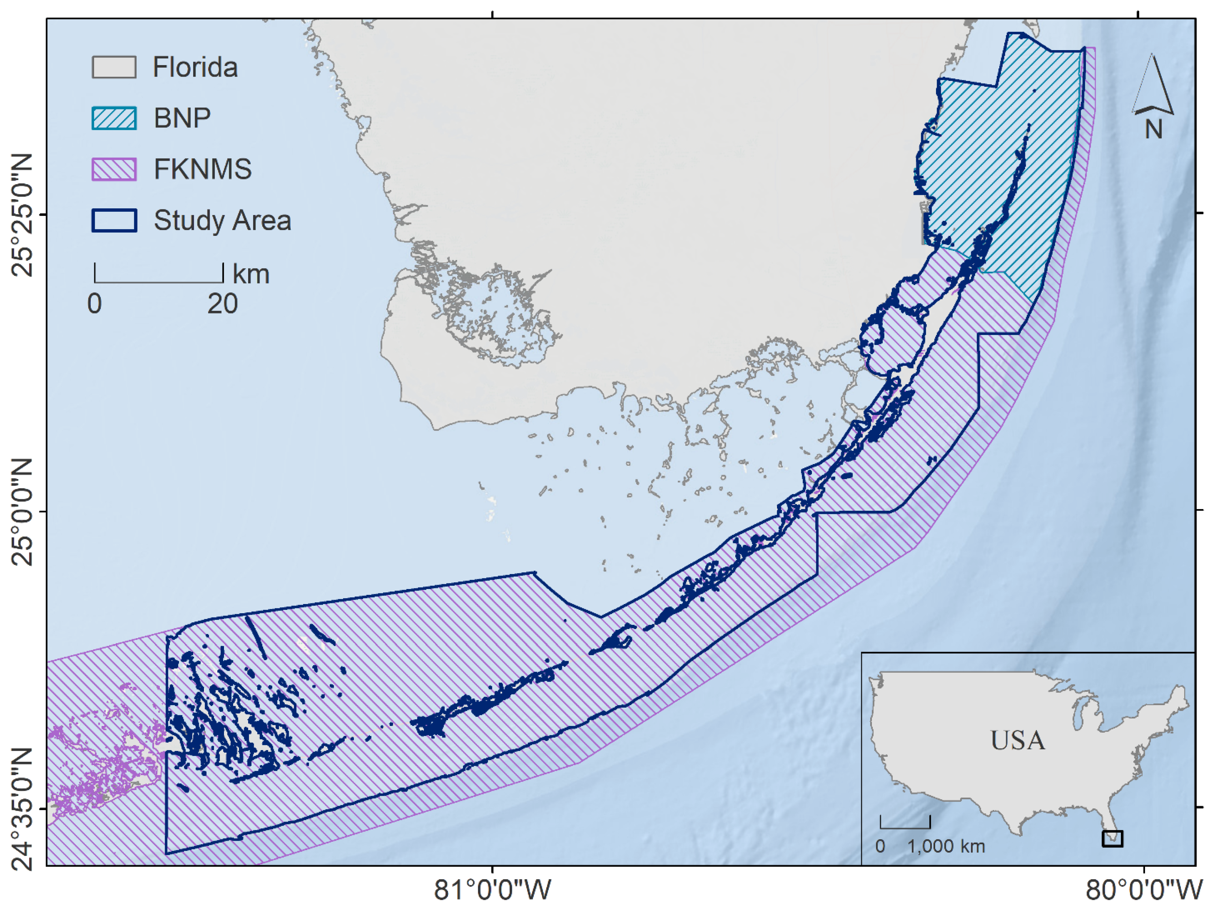
The Florida Keys—a string of islands located off the southern tip of Florida between the Atlantic Ocean and the Gulf of Mexico—were selected as a case study for this research (Figure 1). The seascape in this region has been described as a mangrove–seagrass–reef continuum featuring patches of shoreline mangroves, dense seagrass beds interspersed with patch reefs, and finally the Florida Reef Tract located 5–15 km offshore [41]. Despite protection from the Florida Keys National Marine Sanctuary (FKNMS) and Biscayne National Park (BNP), this region has experienced significant declines in biogenic habitat over the last 50 years. A range of local, state, and federal organizations are now focusing substantial resources on habitat restoration to combat loss and fragmentation, with the offshore reef tract being a major target [42]. These restoration efforts will benefit from a thorough understanding of the daily, seasonal, and ontogenetic migrations of reef fishes between spatially isolated habitats across the seascape, as these movements increase reef productivity and resilience through the transfer of nutrients, the maintenance of top-down control on coral predators, and the enhancement of grazing pressure on harmful epiphytes and macroalgae that could otherwise shift reefs into a macroalgal state [43,44,45]. In fact, the transfer of nitrogen and phosphorus from sheltering resident and migratory reef fishes to their host corals has been demonstrated to significantly increase zooxanthellae abundance and coral growth rates [46,47]. Fish-derived nutrient hotspots thus offer important supplements to oligotrophic tropical and subtropical coral reefs, including those of the Florida Keys [48]. Therefore, we focused on modeling habitat suitability for reef fishes in the coastal region (≤50 m depth) from Key Biscayne in the Upper Keys to Cudjoe Key in the Lower Keys.
2.2. Focal Species
We selected gray snapper (Lutjanus griseus) and bluestriped grunt (Haemulon sciurus) as focal species due to their complex, multi-habitat life histories. Though generally considered reef-associated as adults, these species occupy spatially discrete patches of varying habitat type through ontogeny, resulting in them being categorized as seascape nursery species [49,50]. In Southern Florida, larval L. griseus and H. sciurus settle in seagrass beds around September and February, respectively, before expanding to mangroves several months later [51]. Juveniles often remain in nearshore nurseries for months to years, then, as sub-adults, undertake a cross-shelf migration to join adults on offshore coral reefs. Although it is clear that their ontogenetic migrations play an important role in maintaining seascape-wide ecological connectivity, there remains a paucity of information on habitat suitability across the seascape for L. griseus and H. sciurus. Additionally, there may be considerable inter-species variation in habitat suitability, and consequently, functional connectivity, stemming from unique preferences for nearshore strata [51,52], tolerances to salinity fluctuation [53], and motivations for movement [54,55]. Addressing these knowledge gaps is of critical importance as L. griseus and H. sciurus play key ecological and economic roles in the region as abundant members of the fish assemblage, highly mobile predators and vectors of nutrient transfer, and valued sport and commercial fishery targets [56,57].
Data describing the size, abundance, and distributions of L. griseus and H. sciurus were obtained from two multi-agency monitoring programs coordinated by the NOAA Southeast Fisheries Science Center: the South Florida Reef Visual Census (RVC) and the Mangrove Visual Survey (MVS). Using a two-stage stratified random sampling design, the RVC program surveys fish communities on coral reefs and other hard bottom habitats biennially using a stationary visual survey method [58]. Similarly, the MVS program conducts annual belt transect surveys alongside randomly selected mangrove shoreline sites in Biscayne Bay, Card Sound, Barnes Sound, and northeastern Florida Bay [59,60]. At each site, a trained diver records the identity, abundance, and size structure of all fishes encountered; RVC surveys occur within a 7.5 m-radius imaginary cylinder extending vertically from the seafloor to the surface, while MVS surveys take place over 30 × 2 m transects established parallel to the shore. These programs were designed to collect data that enables the detection of spatiotemporal changes in reef fish species composition, size, and abundance using statistical analyses. Thus, we compiled RVC and MVS data collected at unique sampling sites in 2014, 2016, and 2018 to maximize the spatial coverage of georeferenced L. griseus and H. sciurus records. This process also ensured a temporal match between the two reef fish monitoring programs and the spatial predictors described below, which are based largely on data collected between 2014 and 2018. Considering the dynamic nature of the Florida Keys, where seafloor features change over time, we used temporal data alignment to prevent model inaccuracies.
2.3. Spatial Predictors
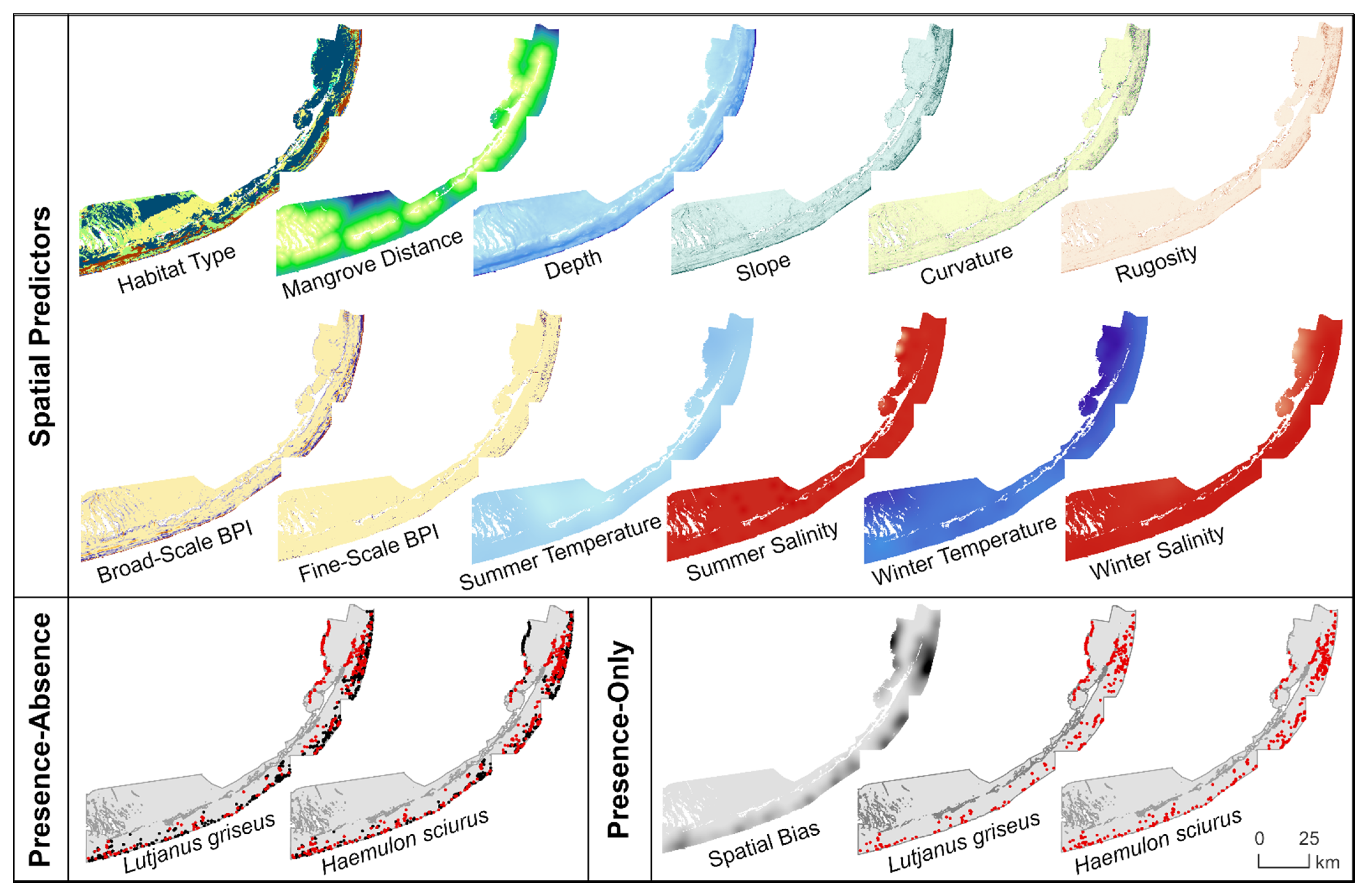
To explore the relationship between spatial predictors and L. griseus and H. sciurus distributions, we constructed raster data layers to map the following environmental categories: benthic habitat, bathymetry and seafloor morphology, and water conditions (Table 1, Figure 2). All rasters had an interpolated resolution of 5 × 5 m and were referenced to the Florida East projected coordinate system and the NAVD vertical coordinate system where applicable.
2.3.1. Benthic Habitat
Benthic habitat data were obtained from Florida’s Unified Reef Map v2.0 [61], a seamless map of benthic habitats from Martin County to the Dry Tortugas derived from remote sensing imagery, high-resolution bathymetric data, and in situ observations using a five-tier hierarchical classification system. We supplemented the Reef Map with a separate GIS dataset of shoreline mangroves to fully capture the extent of this potentially important nursery habitat [62]. For this research, we used Level 1 map classifications, which delineate the major benthic habitat types while maintaining agreement between the Reef Map’s contributing agencies. Habitat data were rasterized, producing cells that reflected the IDs of 12 possible benthic habitats: individual or aggregated patch reef, scattered coral and rock in unconsolidated sediment, continuous seagrass, discontinuous seagrass, unconsolidated sediment, aggregate reef, pavement, reef rubble, mangrove, artificial, dredged and excavated, and ridge. We also assessed the importance of mangrove nursery proximity by constructing a raster of Euclidean distances to the nearest mangrove habitat using the raster R package (v3.3–13) [63] in R version 4.0.2 [64].
2.3.2. Bathymetry and Seafloor Morphology
NOAA’s 1/9th ArcSecond Resolution Continuously Updated Digital Elevation Model served as an initial bathymetric surface for this research [65]. Seafloor morphology was quantified from the bathymetric surface by applying metrics of slope, curvature, rugosity, bathymetric position index (BPI), and standard deviation of depth using the Benthic Terrain Modeler ArcGIS extension (BTM v3.0) [66] in ArcGIS v10.7.1. These rasters captured detailed information on the structure and complexity of the seafloor, including the locations of crests, flats, and valleys, the direction of benthic flow, and the roughness of the local surface [67]. The influence of seascape surface morphology on the distribution of tropical reef fishes has been demonstrated in coral reef ecosystems in the U.S. Caribbean [68,69], Hawaii [29,70,71], and elsewhere [72]; however, this approach has not been applied at a seascape scale to fishes of the Florida Keys.
2.3.3. Water Conditions
Seasonal water conditions, in addition to habitat availability and seafloor morphology, may play a role in shaping the distributions of L. griseus and H. sciurus. We investigated this possibility using raster data layers of mean bottom temperature, salinity, and dissolved oxygen. Using the gstat R package (v2.0–6) [73], we interpolated water quality data from sites that were sampled regularly over the 2014–2018 period by the Southeast Environmental Research Center’s Water Quality Monitoring Network and the Miami-Dade County Surface and Groundwater Quality Viewer. Our research focused on two critical seasons—winter (January–March) and summer (July–September)—to capture not only annual extremes, but also important periods in the life histories of L. griseus and H. sciurus, including habitat expansion and spawning activity [51,74,75].
2.4. Model Development
2.4.1. Filtering and Partitioning of Occurrence Records
As functional connectivity for L. griseus and H. sciurus across the Florida Keys seascape is maintained primarily by the cross-shelf (5–15 km) ontogenetic migrations of their sub-adult life stage, we focused our habitat suitability modeling efforts specifically on this subpopulation. Therefore, we restricted L. griseus and H. sciurus records using the size cut-offs defined in a previous Florida study [51], where sub-adults are those between the size at year 1 and the size at maturation (Table 2). Prior to habitat suitability modeling, species occurrence records were partitioned into calibration (70%) and evaluation (30%) subsets following a random split approach (Table 2).
2.4.2. Selection of Spatial Predictors
Pearson correlation coefficients (r) and variance inflation factors (VIF) were used to assess collinearity among the environmental raster data layers using thresholds of |0.7| and 5 for r and VIF scores, respectively [76]. Four spatial predictors were removed due to multicollinearity issues—standard deviation of depth, plan curvature, and dissolved oxygen across both seasons. Of the 12 predictors retained for modeling, the highest correlation was between summer and winter salinities (r = 0.61) and the largest VIF score, belonging to depth, was 2.63 (Supplementary Table S1 and Supplementary Figure S2).
2.4.3. Penalized Logistic Regressions
Penalized logistic regressions predicting habitat suitability for sub-adult L. griseus and H. sciurus were constructed in R using the glmnet (v4.1.1) [77] and caret (v6.0.86) [78] packages, in R version 4.0.2. [64]. For each species, two logistic regressions were fit via penalized maximum likelihood. The first set of models applied the lasso penalty (i.e., L1-regularization, alpha = 1), a method that minimizes the absolute magnitude of the regression coefficients [79]. The lasso penalty reduces variance by shrinking or assigning a value of zero to some coefficients, thereby finding the optimal balance between model fit and complexity. The second set of models applied the ridge penalty (i.e., L2-regularization, alpha = 0), a method that minimizes the sum of the squared coefficients [80]. Unlike lasso, the coefficients in ridge regression can only asymptotically approach a value of zero. We applied these penalty terms independently to determine whether predictive performance varies based on regularization strategy.
The appropriate shrinkage parameters (lambda) for lasso and ridge were determined based on 10-fold cross validation using the cv.glmnet function of the glmnet package [77]. Penalized logistic regressions were then fit for each species separately using caret, again using 10-fold cross validation for model calibration. Thus, each model was fit using the 70% of presence–absence records set aside for model calibration and the 12 spatially explicit environmental predictors. Finally, the fitted training models were used to extrapolate predictions across the study area via the predict function of the R package raster [63].
2.4.4. MaxEnt Models
Maximum entropy models predicting relative habitat suitability for sub-adult L. griseus and H. sciurus were constructed using MaxEnt version 3.4.1. [81]. MaxEnt automatically applies L1-regularization to find the most parsimonious model [35,82]. The default regularization multiplier is 1.0, however, we used species-specific tuning to identify the regularization value and feature classes (i.e., functions of continuous environmental covariates) that enhanced predictive ability while minimizing overfitting [83,84]. After comparing five potential regularization multipliers (0.25, 0.5, 1.0, 2.0, and 5.0) using the ENMEval R package (v0.3.1) [85], it was determined that a value of 5.0, in combination with linear, quadratic, and hinge features, was optimal for constructing presence-background HSMs for sub-adult L. griseus and H. sciurus. Additionally, to prevent environmental bias stemming from spatially biased occurrence data [86,87], we created a Gaussian kernel density surface to capture the distribution of RVC and MVS sampling effort. This bias grid was fed into MaxEnt via the “bias file” option, enabling the sampling distribution to be factored out during construction of the training algorithm.
MaxEnt models were constructed using the 12 spatially explicit environmental predictors and the 70% of presence-only records designated for model calibration. Initial tuning and subsequent modeling were conducted using 10-fold cross validation and a set of 10,000 background points selected according to the bias file described above. The complementary log–log (cloglog) transformation was used, producing surfaces that reflected the predicted relative habitat suitability (or relative likelihood of occurrence) on a scale of 0 to 1.
2.5. Model Assessment
2.5.1. Discriminatory Ability
Predictive performance was compared between penalized logistic regression and MaxEnt models using the area under the receiver-operator curve (AUC). AUC is a threshold-independent, rank-based statistic that indicates a model’s ability to discriminate between a random absence (or background) point and a random presence point [35]. By assessing model performance over a variety of thresholds, the AUC test statistic provides an indication of discriminatory ability on a continuous scale and enables comparisons between modeling algorithms. AUC values range from 0 to 1, with the latter representing perfect discrimination. AUCs ≤ 0.5 suggest random or worse than random performance [88].
2.5.2. Binary Predictive Performance
We assessed the binary classification accuracy of each model using the 30% of presence–absence records set aside during the initial train–test split. The predicted suitability surfaces for each species were first discretized to a binary scale using a standard threshold of 0.5 for the predicted probability (penalized regression) or relative likelihood (MaxEnt) of presence. A confusion matrix was then calculated for each species–model combination, and the accuracy, sensitivity (i.e., percentage of correctly predicted presences), and specificity (i.e., percentage of correctly predicted absences) were examined. Though this standard threshold enables a general comparison of map accuracy between modeling algorithms, it may not represent the suitability cut-off at which the models optimally distinguish between suitable and unsuitable locations, which is an essential goal when defining nodes for subsequent connectivity modeling. Thus, we also identified the suitability thresholds at which each model achieved a maximum sum of sensitivity plus specificity (max SSS). Max SSS provides an indication of how conservative of a suitability cut-off must be used to maximize discrimination between the presence and absence (or suitable and unsuitable) locations [89].
2.5.3. Variable Importance
Variable importance scores were also calculated for each species across the three modeling techniques. For penalized logistic regressions built using glmnet and caret, variable importance was assessed using varImp, a function of the caret package that scales variables from 0 to 100 according to the absolute value of their standardized coefficients. For MaxEnt models, jackknife resampling was used to assess the influence of each predictor, this procedure sums the change in regularized gain (i.e., a goodness of fit measure based on a variable’s ability to distinguish species presence sites) across the ten cross validation folds. Regardless of model type, larger values indicate a higher level of importance.
3. Results
3.1. Discriminatory Ability
We used the AUC test statistic to determine whether penalized logistic regression and MaxEnt modeling techniques differ in their ability to discriminate between suitable and unsuitable locations across a variety of thresholds. According to the AUC statistic, regularization strategy had little effect on the discriminatory ability of regression HSMs, as lasso- and ridge-penalized models displayed similar performance within species. For sub-adult L. griseus, both penalized regressions achieved an AUC value of 0.74, indicating a good model fit. Discriminatory ability improved slightly for penalized regressions of sub-adult H. sciurus suitability, with lasso and ridge regressions producing AUCs of 0.76 and 0.75, respectively. However, regardless of the regularization strategy, the penalized logistic models were outperformed by MaxEnt, which yielded AUC values of 0.88 for L. griseus and 0.86 for H. sciurus (Table 3).
3.2. Binary Predictive Performance
To produce the discrete patches of suitable habitat (i.e., nodes) required for modeling potential connectivity, the continuous habitat suitability surfaces must be discretized to a binary scale. Therefore, we used confusion matrices to assess each model’s binary predictive performance following discretization at two thresholds. When first discretized using a standard suitability cut-off of 0.5 and compared to the withheld validation data, lasso and ridge HSMs for sub-adult L. griseus achieved classification accuracies of 77.9% and 77.7%, respectively. Map accuracy was slightly lower for sub-adult H. sciurus, with values of 73.2% and 74.2% for lasso and ridge regressions, respectively. Relative to the penalized regressions, overall map accuracy for MaxEnt was low when assessed at this suitability cut-off, ranging from roughly 40–50% (Table 3). The models also varied in terms of sensitivity and specificity, with penalized regressions successfully identifying known absence (i.e., unsuitable) locations more frequently than known presence (i.e., suitable) locations and MaxEnt following the opposite trend.
The max SSS threshold selection strategy, which optimizes discrimination between known presence and absence localities, identified substantially different suitability cut-offs for each of the modeling algorithms (Table 3). In general, the penalized logistic models would have to lower their suitability thresholds to roughly 0.30 to maximize discrimination, whereas the MaxEnt models optimized discrimination between known presence and absence sites at a threshold of 0.65, a far less conservative cut-off. Although the overall map accuracy of the MaxEnt models still trailed those of the penalized regressions, the percentage of correctly predicted presence locations (i.e., sensitivity) was higher for MaxEnt than nearly all regressions. Additionally, discretization using max SSS thresholds increased the balance between sensitivity and specificity across all species–model combinations.
3.3. Variable Importance
To better understand the species–seascape interactions driving patterns of habitat suitability and, consequently, potential connectivity, we examined the continuous habitat suitability surfaces and variable importance plots produced by each model. Within species, there was a high level of agreement between the habitat suitability predictions of the three modeling techniques; however, lasso- and ridge-penalized regressions predicted smooth, gradual patterns of decreasing suitability as distance from shore increased, whereas MaxEnt captured patchy distributions of suitable habitat with noticeable fine-scale differences (Supplementary Figure S3). Furthermore, the models revealed species-specific responses to the various spatial predictors, resulting in considerable inter-species variation in predicted suitability across the seascape (Figure 3). For brevity, we focus here only on the variable contributions of the top-performing continuous HSM for each species (i.e., the MaxEnt models); variable importance information for the penalized regressions is provided in Supplementary Figure S4 and response curves for the top five MaxEnt predictors are provided in Supplementary Figure S5.
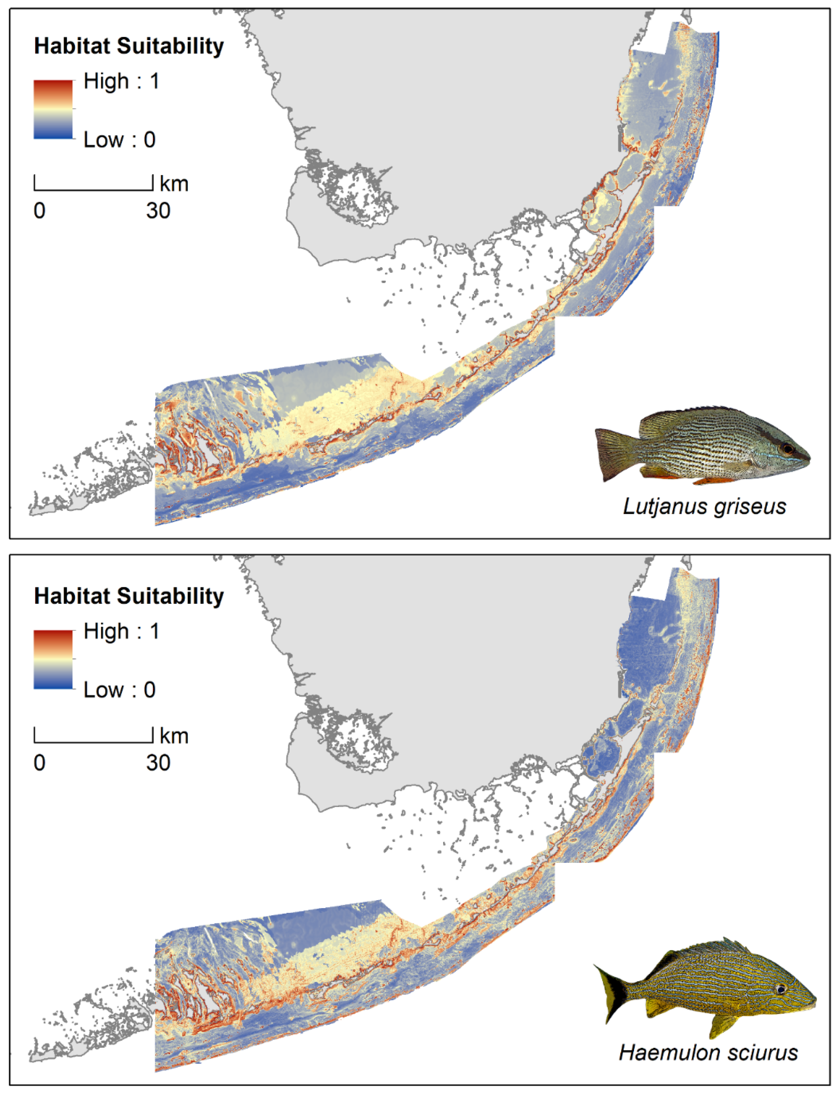
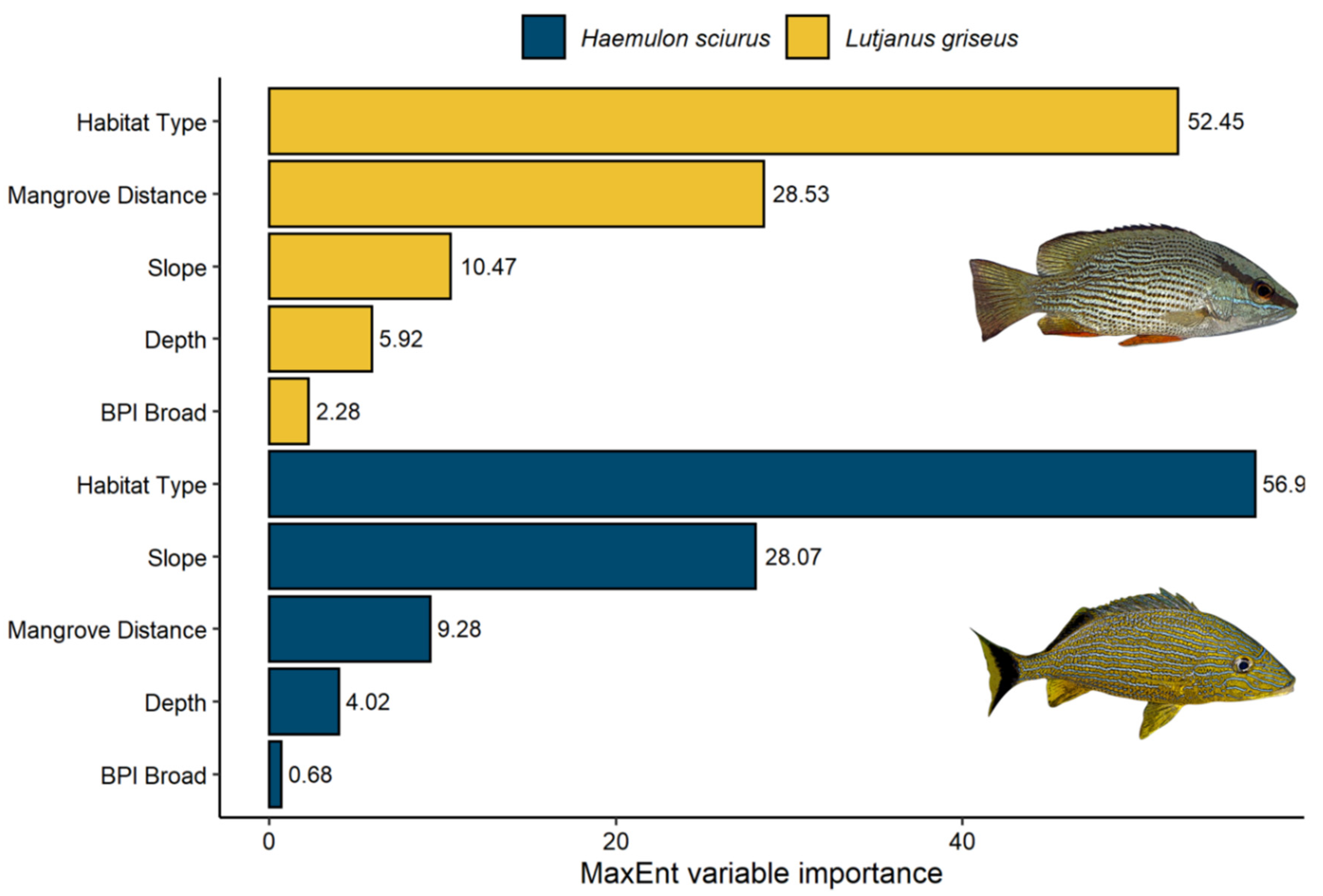
For sub-adult L. griseus, MaxEnt’s jackknife procedure identified benthic habitat type as the single most influential predictor of habitat suitability, followed by Euclidean distance to the nearest mangrove, slope, depth, and broad-scale BPI (Figure 4, Supplementary Figure S5). Predicted habitat suitability for L. griseus was high in shallow waters (<5 m depth) within roughly 200 m from mangroves, with the highest values predicted at the interface of shoreline mangroves and seagrass meadows (i.e., the seagrass fringe). Patches of high suitability were also identified along the shoreward side of the barrier reef tract, primarily in areas of increasing slope (>5 degrees) and over aggregate reefs and isolated patch reefs with shallow peaks surrounded by dense seagrass (Figure 3). In contrast, unconsolidated sediment and discontinuous seagrass were predicted to have the lowest relative likelihood of sub-adult L. griseus presence. Broad-scale BPI positively influenced predicted suitability levels, with broad peaks and ridges favored over flats and valleys. Though their roles were negligible relative to the top five predictors, mean winter salinity and mean summer temperature both showed negative relationships with predicted suitability when used in isolation. The remaining predictors—curvature, rugosity, fine-scale BPI, mean summer salinity, and mean winter temperature—were assigned a variable importance score of zero.
The five most influential predictors regulating the distribution of suitable habitat for sub-adult H. sciurus were benthic habitat type, slope, Euclidean distance to the nearest mangrove, depth, and broad-scale BPI (Figure 4, Supplementary Figure S5). Similar to the L. griseus model, predicted habitat suitability for sub-adult H. sciurus was high along the seagrass fringe and over individual patch reefs and aggregate coral reefs, especially those with broad peaks (Figure 3). However, relative to the L. griseus model, MaxEnt predicted higher suitability levels for H. sciurus over ridges and in patches of pavement, scattered rock, and reef rubble, and lower suitability levels in seagrass with the exception of those in shallow areas immediately adjacent to mangroves. Although depths shallower than 5 m were predicted to be the most suitable, the relative likelihood of H. sciurus presence remained above 50% at depths down to roughly 25 m. Predicted habitat suitability for H. sciurus also declined rapidly as Euclidean distance from the nearest mangrove approached 200 m, however, suitability levels for this species began gradually increasing again at a distance of around 1 km rather than continuing to decline. Furthermore, the mangrove shorelines on the windward and leeward sides of the Florida Keys had consistently higher estimates of habitat suitability than those along the mainland in Biscayne Bay (Figure 3). Although this trend was also visible in the L. griseus model, it was much more pronounced for H. sciurus. Water conditions contributed only weakly to overall model fit, however, there were positive relationships between the relative likelihood of sub-adult H. sciurus presence and mean winter salinity and temperature. In contrast, curvature, rugosity, fine-scale BPI, and mean summer salinity and temperature had contribution scores of zero.
4. Discussion
4.1. Model Performance
We compared penalized logistic regression and MaxEnt models of habitat suitability for two economically and ecologically critical reef fish species in the Florida Keys, USA, with the goal of identifying which modeling algorithm produces the most realistic and detailed products for use in subsequent connectivity modeling. MaxEnt’s AUC values were consistently higher than those of either the lasso- or ridge-penalized logistic regressions, suggesting that MaxEnt was better able to distinguish between suitable and unsuitable locations for sub-adult L. griseus and H. sciurus when evaluated across a range of suitability thresholds. Although the overall accuracy of the MaxEnt models fell below those of the penalized regressions when discretized using standard and max SSS suitability thresholds, MaxEnt produced similar or improved sensitivity estimates relative to the penalized regressions. MaxEnt’s consistently high sensitivity values suggest that these models were able to reliably identify known presence locations, which is essential for delineating the suitable habitat nodes required to produce spatial graphs for connectivity assessment. The high-resolution suitability maps produced by MaxEnt also appear to be better suited for conversion to resistance surfaces, as these models predicted patchy distributions of suitable habitat across the seascape that more closely aligned with the known ecology of the study species, as described below in Section 4.2.
Consistent with our findings, MaxEnt’s predictive performance has paralleled or exceeded that of other machine learning and regression techniques in several comparative studies. For instance, MaxEnt and penalized logistic regression techniques yielded similar AUC values when used to model the distributions of several tree species in Spain, with both models outperforming standard logistic regressions [90]. Similarly, MaxEnt achieved the highest predictive performance out of five modeling methods when used to model habitat suitability for the invasive Argentine ant across the Iberian Peninsula, producing predictive distributional maps that highlighted areas susceptible to invasion [39]. MaxEnt has even performed well in spatially and topographically complex seascapes, as demonstrated by a comparative study of ten presence-only modeling algorithms applied to demersal fish species of Australia [91]. Our research, therefore, joins these and other examples from the literature that illustrate MaxEnt’s usefulness as a tool for mapping species distributions across a range of taxa and environmental settings, especially in scenarios where distributional patterns are thought to be driven by complex species–environment relationships. These results can likely be attributed to MaxEnt’s ability to harness categorical data and linear, quadratic, hinge, and threshold functions of continuous environmental variables, while simultaneously maintaining a balance between model fit and complexity using regularization [82]. Despite its growing promise and popularity among ecologists, attempts to leverage MaxEnt products for connectivity modeling remain scarce.
4.2. Variable Importance
Of the 12 environmental predictors assessed in our study, habitat type was identified as the main driver of suitability for sub-adult L. griseus and H. sciurus, with dense seagrass beds, shoreline mangroves, patch reefs, and shoreward aggregate reefs being especially important. According to our models, these habitats play a variable role in supporting sub-adult L. griseus and H. sciurus, depending on their geographic location. This trend was especially apparent for shoreline mangroves, with suitability predicted to be highest in mangroves along the leeward and windward sides of the Keys and surrounding Biscayne Bay’s southern islands. Previous research in the region revealed a similar pattern of habitat use whereby sub-adult L. griseus and H. sciurus selected for easterly mangroves along the Keys, whereas larger-bodied adults were more common in Biscayne Bay’s expansive mainland forests [51,52]. The high suitability levels predicted along the seagrass fringe and in areas within several hundred meters of a nearby mangrove shoreline likely reflect the regular diel migrations of grunts and snappers between daytime resting sites in mangroves and nocturnal foraging grounds in seagrass meadows, which cover distances of up to 1 km [51,92,93]. Furthermore, patch reefs and sections of the reef tract adjacent to lush seagrass beds and mangrove shorelines, particularly those along the Keys, were predicted to have a higher relative likelihood of presence for both species compared to those located alongside unvegetated substrates. Together, these results suggest that patch reefs serve as critical stepping-stones connecting mangrove and seagrass nurseries to adult habitat on offshore reefs. However, sub-adult dispersal between back reef habitats may be limited to only immediately accessible patches of topographically complex habitat, with implications for the replenishment of adult populations across the barrier reef tract [94,95]. These findings also suggest that nutrient supplementation and top-down control of coral predators by migratory reef fishes may be greatest in patch reef, back reef, and reef crest communities neighboring seagrasses and mangroves, with consequences for coral growth and the placement of coral restoration efforts [44,48].
Beyond the type and spatial arrangement of benthic habitats, suitability varied as a function of depth and seafloor surface morphology, as quantified by slope and bathymetric position index (BPI). Generally, the likelihood of L. griseus and H. sciurus presence decreased with increasing depth, with this pattern being especially abrupt for L. griseus. The predicted suitability maps also displayed within-patch variation, with both species responding positively to even small increases in slope (<5 degrees). Additionally, our models revealed that the influence of BPI on habitat suitability is both scale- and species-dependent, with broad-scale BPI having a stronger influence over predicted suitability levels for L. griseus than H. sciurus. Nonetheless, fine-scale BPI and two other fine-scale metrics of seafloor surface complexity—curvature and rugosity—were dropped entirely from both MaxEnt models. These results indicate that the distributions of sub-adult L. griseus and H. sciurus across the seascape are primarily driven by broad-scale habitat features and geographic location, a finding that is consistent with previous research on predatory reef fishes and which may be related to the high vagility and large home range sizes of these species (1–5 km) [96,97,98,99]. However, previous work in the Caribbean revealed that seafloor morphology and geographic location interact to drive the distributional patterns of herbivores, in addition to invertivores and piscivores, suggesting that this trend is likely common across coastal reef fish communities rather than being restricted to mobile predators [68].
Although neither salinity nor temperature acted as a major determinant of suitability, these variables acted as filters to mediate the relative suitability of otherwise similar habitats. Previous research has demonstrated significant inter-species variation in salinity tolerances, with L. griseus being abundant in low-to-intermediate salinities and H. sciurus being abundant in stable, high salinities [53,100]. These relationships were reflected in MaxEnt’s predictions and were especially noticeable in Biscayne Bay, where salinity fluctuates significantly as a result of both freshwater discharge and tidal exchange. As such, the western and southwestern mainland coasts, which are characterized by extreme salinity fluctuations and lower overall means [59], were predicted to have higher suitability levels for L. griseus than H. sciurus. In contrast, habitats along the leeward and windward sides of the Upper Keys that have narrow salinity ranges dominated by seawater were predicted to have higher suitability levels for H. sciurus. Additionally, the present finding that relative suitability for sub-adult L. griseus decreases rapidly as summer temperatures approach 31 °C is in agreement with previous laboratory experiments that estimated 33 °C as being close to the maximum for juvenile gray snapper feeding [101]. Considering that settlement and grow-out occur from summer through early fall [51], this temperature constraint may be an artifact of juvenile habitat selection. On the other hand, the positive relationship between mean winter temperature and predicted suitability for sub-adult H. sciurus may reflect the winter spawning and settlement behavior of this species, as warmer winter temperatures decrease the overwinter mortality of juveniles and increase the chances of successful sub-adult dispersal to the offshore reefs [102,103].
4.3. Implications for Seascape Connectivity Modeling and Conservation
Based on our case study, habitat composition and arrangement, depth, and broad-scale bathymetric features are among the most important factors to consider when planning conservation efforts for reef fish species with complex, multi-habitat life histories. In particular, our models highlight the value of targeting mosaics of interconnected habitats, rather than single biotopes, when planning marine protected areas, reserve networks, and resource management [13,14,104]. The importance of considering surrounding seascape context and connectivity is not limited to the protection and conservation of existing ecosystems, but also to the restoration of degraded and fragmented habitats. By strategically placing restoration activities within the seascape, restoration practitioners can enhance intra- and inter-habitat connectivity, thereby increasing dispersal and harnessing key ecological processes including herbivory and primary production, predation and secondary production, and nutrient turnover [44]. Although the application of seascape connectivity as a spatially explicit metric in restoration planning has been limited thus far, projects that have incorporated surrounding seascape context in their site selection process have seen positive outcomes [105]. Integrative approaches that combine the strengths of habitat suitability modeling and connectivity modeling are becoming increasingly common and accessible thanks to improvements in data availability and the development of decision support tools like Marxan Connect and Zonation [15,24].
In conclusion, our research demonstrates that MaxEnt, a presence-background machine learning approach, outperforms traditional presence–absence techniques in terms of predictive performance and ability to produce habitat suitability maps that reflect the known ecology of sub-adult L. griseus and H. sciurus in the Florida Keys. These results are consistent with previous terrestrial studies that have found similar or improved predictive performance of MaxEnt relative to standard or penalized logistic regressions [37,90,106]. Furthermore, our research, coupled with previous work on warm-water kelps [107], demersal fishes [91], and shallow and deep-sea corals [108,109], demonstrate that MaxEnt’s promise as a fast, open-source tool for mapping species distributions extends beyond the land–sea interface. Although analogs exist from the terrestrial literature (e.g., [26,30]), the application of habitat suitability modeling as a precursor to marine connectivity assessments and conservation planning remains scarce. We anticipate that MaxEnt-derived nodes and linkages can be combined with data on species biological traits to produce detailed and ecologically realistic spatial graphs for connectivity assessment. As a next step, we plan to construct and operationalize these graphs for habitat restoration planning through scenario testing, including the iterative addition or removal of nodes and linkages (i.e., restoration and fragmentation scenarios, respectively). As habitat restoration efforts ramp up across the spatially and topographically complex seascape of the Florida Keys, we encourage restoration practitioners and coastal managers to adopt a multi-step site selection strategy that harnesses the strengths of both habitat suitability and connectivity modeling.
Supplementary Materials
The following are available online at https://0-www-mdpi-com.brum.beds.ac.uk/article/10.3390/d13100465/s1, Table S1: Variance inflation factors, Figure S1: Pearson pairwise correlation matrix of all available spatial predictors, Figure S2: Pearson pairwise correlation matrix of spatial predictors retained for habitat suitability modeling, Figure S3: Lasso-penalized logistic regression, ridge-penalized logistic regression, and MaxEnt predictions of habitat suitability for sub-adult gray snapper (Lutjanus griseus) and bluestriped grunt (Haemulon sciurus) in the Florida Keys, USA, Figure S4: Plots of the top five most influential predictors of sub-adult gray snapper (Lutjanus griseus) and bluestriped grunt (Haemulon sciurus) suitability according to lasso- and ridge-penalized logistic regressions, Figure S5: MaxEnt response curves for the top five predictors of habitat suitability for sub-adult gray snapper (Lutjanus griseus) and bluestriped grunt (Haemulon sciurus) in the Florida Keys, USA.
Author Contributions
Conceptualization, C.E.S., L.M.W., S.J.P. and S.J.G.; Methodology, formal analysis and investigation, C.E.S.; Writing—original draft preparation, C.E.S.; Writing—review and editing, C.E.S., L.M.W., S.J.P. and S.J.G.; Visualization, C.E.S.; Supervision, S.J.G.; Project administration, C.E.S. and S.J.G.; Funding acquisition, S.J.G. All authors have read and agreed to the published version of the manuscript.
Funding
This research and the associated APC were funded by the Canada Research Chairs Program, NSERC Discovery Grant RGPIN-2018-05712, and a Sloan Science Fellowship to S.J.G. Additional funding to C.E.S. was provided by the University of Alberta Graduate Fellowship and the Alberta Graduate Excellence Scholarship.
Institutional Review Board Statement
Not applicable.
Data Availability Statement
Data, R scripts, MaxEnt command line code, and ArcGIS geoprocessing workflows associated with this research are available online at https://github.com/CourtneyStuart/FL_Habitat_Suitability (accessed on 30 September 2020). Reef fish occurrence records were obtained from two public data sources: the South Florida Reef Visual Census (https://grunt.sefsc.noaa.gov/rvc_analysis20/strata/index (accessed on 30 September 2020) or https://github.com/jeremiaheb/rvc (accessed on 30 September 2020)) and the Mangrove Visual Survey (https://www.ncei.noaa.gov/access/metadata/landing-page/bin/iso?id=gov.noaa.nodc:0159580 (accessed on 30 September 2020)). The Florida Keys National Marine Sanctuary and Biscayne National Park GIS shapefiles used for mapping are accessible at https://sanctuaries.noaa.gov/library/imast_gis.html (accessed on 30 September 2020) and https://public-nps.opendata.arcgis.com/datasets/nps-boundary-1/data (accessed on 30 September 2020), respectively. The water quality data used in this research were provided by the Miami-Dade County Surface and Groundwater Quality Viewer (https://mdc.maps.arcgis.com/apps/webappviewer/index.html?id=3fd24515ee614f5db63924d7323a4ea7 (accessed on 30 September 2020)) and the SERC-FIU Water Quality Monitoring Network, which is supported by EPA Agreement #X7 00D02412-1 and NOAA Agreement #NA09NOS4260253 (http://serc.fiu.edu/wqmnetwork/FKNMS-CD/index.htm (accessed on 30 September 2020)). Please email C.E.S. if you would like access to the large spatial data layers produced during this research.
Acknowledgments
We thank Joe Serafy and Jeremiah Blondeau of the NOAA Southeast Fisheries Science Center and Alejandro Acosta of the Florida Fish and Wildlife Conservation Commission—Fish and Wildlife Research Institute for their assistance acquiring and interpreting reef fish occurrence data, without which this research would not have been possible. We also extend our gratitude to two anonymous reviewers, whose comments on an earlier draft helped to improve the quality of our manuscript.
Conflicts of Interest
S.J.P. is director of Seascape Analytics Ltd. and declares no financial relationships or other potential conflict of interest. The remaining authors (C.E.S., L.M.W., S.J.G.) declare no conflict of interest.
References
- Marshall, C.E.; Glegg, G.A.; Howell, K.L. Species Distribution Modelling to Support Marine Conservation Planning: The next Steps. Mar. Policy 2014, 45, 330–332. [Google Scholar] [CrossRef]
- Villero, D.; Pla, M.; Camps, D.; Ruiz-Olmo, J.; Brotons, L. Integrating Species Distribution Modelling into Decision-Making to Inform Conservation Actions. Biodivers. Conserv. 2017, 26, 251–271. [Google Scholar] [CrossRef]
- Smale, D.A.; Wernberg, T.; Oliver, E.C.J.; Thomsen, M.; Harvey, B.P.; Straub, S.C.; Burrows, M.T.; Alexander, L.V.; Benthuysen, J.A.; Donat, M.G.; et al. Marine Heatwaves Threaten Global Biodiversity and the Provision of Ecosystem Services. Nat. Clim. Chang. 2019, 9, 306–312. [Google Scholar] [CrossRef] [Green Version]
- Gissi, E.; Manea, E.; Mazaris, A.D.; Fraschetti, S.; Almpanidou, V.; Bevilacqua, S.; Coll, M.; Guarnieri, G.; Lloret-Lloret, E.; Pascual, M.; et al. A Review of the Combined Effects of Climate Change and Other Local Human Stressors on the Marine Environment. Sci. Total Environ. 2021, 755, 142564. [Google Scholar] [CrossRef] [PubMed]
- Polidoro, B.A.; Carpenter, K.E.; Collins, L.; Duke, N.C.; Ellison, A.M.; Ellison, J.C.; Farnsworth, E.J.; Fernando, E.S.; Kathiresan, K.; Koedam, N.E.; et al. The Loss of Species: Mangrove Extinction Risk and Geographic Areas of Global Concern. PLoS ONE 2010, 5, e10095. [Google Scholar] [CrossRef]
- Waycott, M.; Duarte, C.M.; Carruthers, T.J.B.; Orth, R.J.; Dennison, W.C.; Olyarnik, S.; Calladine, A.; Fourqurean, J.W.; Heck, K.L.; Hughes, A.R.; et al. Accelerating Loss of Seagrasses across the Globe Threatens Coastal Ecosystems. Proc. Natl. Acad. Sci. USA 2009, 106, 12377–12381. [Google Scholar] [CrossRef] [PubMed] [Green Version]
- Gardner, T.A.; Côté, I.M.; Gill, J.A.; Grant, A.; Watkinson, A.R. Long-Term Region-Wide Declines in Caribbean Corals. Science 2003, 301, 958–960. [Google Scholar] [CrossRef] [Green Version]
- Deegan, L.A.; Johnson, D.S.; Warren, R.S.; Peterson, B.J.; Fleeger, J.W.; Fagherazzi, S.; Wollheim, W.M. Coastal Eutrophication as a Driver of Salt Marsh Loss. Nature 2012, 490, 388–392. [Google Scholar] [CrossRef]
- Duffy, J.E.; Lefcheck, J.S.; Stuart-Smith, R.D.; Navarrete, S.A.; Edgar, G.J. Biodiversity Enhances Reef Fish Biomass and Resistance to Climate Change. Proc. Natl. Acad. Sci. USA 2016, 113, 6230–6235. [Google Scholar] [CrossRef] [Green Version]
- Benkwitt, C.E.; Wilson, S.K.; Graham, N.A.J. Biodiversity Increases Ecosystem Functions despite Multiple Stressors on Coral Reefs. Nat. Ecol. Evol. 2020, 4, 919–926. [Google Scholar] [CrossRef]
- Kennedy, E.V.; Perry, C.T.; Halloran, P.R.; Iglesias-Prieto, R.; Schönberg, C.H.L.; Wisshak, M.; Form, A.U.; Carricart-Ganivet, J.P.; Fine, M.; Eakin, C.M.; et al. Avoiding Coral Reef Functional Collapse Requires Local and Global Action. Curr. Biol. 2013, 23, 912–918. [Google Scholar] [CrossRef] [Green Version]
- Waltham, N.J.; Elliott, M.; Lee, S.Y.; Lovelock, C.; Duarte, C.M.; Buelow, C.; Simenstad, C.; Nagelkerken, I.; Claassens, L.; Wen, C.K.-C.; et al. UN Decade on Ecosystem Restoration 2021–2030—What Chance for Success in Restoring Coastal Ecosystems? Front. Mar. Sci. 2020, 7, 1–5. [Google Scholar] [CrossRef] [Green Version]
- Olds, A.D.; Connolly, R.M.; Pitt, K.A.; Pittman, S.J.; Maxwell, P.S.; Huijbers, C.M.; Moore, B.R.; Albert, S.; Rissik, D.; Babcock, R.C.; et al. Quantifying the Conservation Value of Seascape Connectivity: A Global Synthesis. Glob. Ecol. Biogeogr. 2016, 25, 3–15. [Google Scholar] [CrossRef]
- Carr, M.H.; Robinson, S.P.; Wahle, C.; Davis, G.; Kroll, S.; Murray, S.; Schumacker, E.J.; Williams, M. The Central Importance of Ecological Spatial Connectivity to Effective Coastal Marine Protected Areas and to Meeting the Challenges of Climate Change in the Marine Environment. Aquat. Conserv. Mar. Freshw. Ecosyst. 2017, 27, 6–29. [Google Scholar] [CrossRef] [Green Version]
- Weeks, R. Incorporating Seascape Connectivity in Conservation Prioritisation. PLoS ONE 2017, 12, e0182396. [Google Scholar] [CrossRef] [PubMed]
- Balbar, A.C.; Metaxas, A. The Current Application of Ecological Connectivity in the Design of Marine Protected Areas. Glob. Ecol. Conserv. 2019, 17, e00569. [Google Scholar] [CrossRef]
- Taylor, P.D.; Fahrig, L.; Henein, K.; Merriam, G. Connectivity Is a Vital Element of Landscape Structure. Oikos 1993, 68, 571–573. [Google Scholar] [CrossRef] [Green Version]
- Taylor, P.D.; Fahrig, L.; With, K.A. Landscape connectivity: A return to the basics. In Connectivity Conservation; Crooks, K.R., Sanjayan, M., Eds.; Cambridge University Press: Cambridge, UK, 2006; pp. 29–43. ISBN 978-0-511-75482-1. [Google Scholar]
- Sambrook, K.; Hoey, A.S.; Andréfouët, S.; Cumming, G.S.; Duce, S.; Bonin, M.C. Beyond the Reef: The Widespread Use of Non-Reef Habitats by Coral Reef Fishes. Fish. Fish. 2019, 20, 903–920. [Google Scholar] [CrossRef]
- Grober-Dunsmore, R.; Pittman, S.J.; Caldow, C.; Kendall, M.S.; Frazer, T.K. A Landscape Ecology Approach for the Study of Ecological Connectivity Across Tropical Marine Seascapes. In Ecological Connectivity among Tropical Coastal Ecosystems; Nagelkerken, I., Ed.; Springer: Dordrecht, The Netherland, 2009; pp. 493–530. ISBN 978-90-481-2405-3. [Google Scholar]
- Tischendorf, L.; Fahrig, L. On the Usage and Measurement of Landscape Connectivity. Oikos 2000, 90, 7–19. [Google Scholar] [CrossRef] [Green Version]
- Urban, D.; Keitt, T. Landscape Connectivity: A Graph Theoretic Perspective. Ecology 2001, 82, 1205–1218. [Google Scholar] [CrossRef]
- McRae, B.H.; Hall, S.A.; Beier, P.; Theobald, D.M. Where to Restore Ecological Connectivity? Detecting Barriers and Quantifying Restoration Benefits. PLoS ONE 2012, 7, e52604. [Google Scholar] [CrossRef] [PubMed]
- Daigle, R.M.; Metaxas, A.; Balbar, A.C.; McGowan, J.; Treml, E.A.; Kuempel, C.D.; Possingham, H.P.; Beger, M. Operationalizing Ecological Connectivity in Spatial Conservation Planning with Marxan Connect. Methods Ecol. Evol. 2020, 11, 570–579. [Google Scholar] [CrossRef] [Green Version]
- Guisan, A.; Zimmermann, N.E. Predictive Habitat Distribution Models in Ecology. Ecol. Model. 2000, 135, 147–186. [Google Scholar] [CrossRef]
- Duflot, R.; Avon, C.; Roche, P.; Bergès, L. Combining Habitat Suitability Models and Spatial Graphs for More Effective Landscape Conservation Planning: An Applied Methodological Framework and a Species Case Study. J. Nat. Conserv. 2018, 46, 38–47. [Google Scholar] [CrossRef]
- Stevenson-Holt, C.D.; Watts, K.; Bellamy, C.C.; Nevin, O.T.; Ramsey, A.D. Defining Landscape Resistance Values in Least-Cost Connectivity Models for the Invasive Grey Squirrel: A Comparison of Approaches Using Expert-Opinion and Habitat Suitability Modelling. PLoS ONE 2014, 9, e112119. [Google Scholar] [CrossRef] [Green Version]
- Lepczyk, C.A.; Wedding, L.M.; Asner, G.P.; Pittman, S.J.; Goulden, T.; Linderman, M.A.; Gang, J.; Wright, R. Advancing Landscape and Seascape Ecology from a 2D to a 3D Science. BioScience 2021, 71, 596–608. [Google Scholar] [CrossRef]
- Wedding, L.M.; Jorgensen, S.; Lepczyk, C.A.; Friedlander, A.M. Remote Sensing of Three-Dimensional Coral Reef Structure Enhances Predictive Modeling of Fish Assemblages. Remote Sens. Ecol. Conserv. 2019, 5, 150–159. [Google Scholar] [CrossRef] [Green Version]
- Poor, E.E.; Loucks, C.; Jakes, A.; Urban, D.L. Comparing Habitat Suitability and Connectivity Modeling Methods for Conserving Pronghorn Migrations. PLoS ONE 2012, 7, e49390. [Google Scholar] [CrossRef]
- Penjor, U.; Kaszta, Ż.; Macdonald, D.W.; Cushman, S.A. Prioritizing Areas for Conservation Outside the Existing Protected Area Network in Bhutan: The Use of Multi-Species, Multi-Scale Habitat Suitability Models. Landsc. Ecol. 2021, 36, 1281–1309. [Google Scholar] [CrossRef]
- Green, E.P.; Mumby, P.J.; Edwards, A.J.; Clark, C.D. A Review of Remote Sensing for the Assessment and Management of Tropical Coastal Resources. Coast. Manag. 1996, 24, 1–40. [Google Scholar] [CrossRef]
- Pearce, J.; Ferrier, S. Evaluating the Predictive Performance of Habitat Models Developed Using Logistic Regression. Ecol. Model. 2000, 133, 225–245. [Google Scholar] [CrossRef] [Green Version]
- Guillera-Arroita, G.; Lahoz-Monfort, J.J.; Elith, J.; Gordon, A.; Kujala, H.; Lentini, P.E.; McCarthy, M.A.; Tingley, R.; Wintle, B.A. Is My Species Distribution Model Fit for Purpose? Matching Data and Models to Applications. Glob. Ecol. Biogeogr. 2015, 24, 276–292. [Google Scholar] [CrossRef]
- Phillips, S.J.; Anderson, R.P.; Schapire, R.E. Maximum Entropy Modeling of Species Geographic Distributions. Ecol. Model. 2006, 190, 231–259. [Google Scholar] [CrossRef] [Green Version]
- Phillips, S.J.; Dudík, M. Modeling of Species Distributions with Maxent: New Extensions and a Comprehensive Evaluation. Ecography 2008, 31, 161–175. [Google Scholar] [CrossRef]
- Elith, J.; Graham, C.H.; Anderson, R.P.; Dudík, M.; Ferrier, S.; Guisan, A.; Hijmans, R.J.; Huettmann, F.; Leathwick, J.R.; Lehmann, A.; et al. Novel Methods Improve Prediction of Species’ Distributions from Occurrence Data. Ecography 2006, 29, 129–151. [Google Scholar] [CrossRef] [Green Version]
- Gibson, L.; Barrett, B.; Burbidge, A. Dealing with Uncertain Absences in Habitat Modelling: A Case Study of a Rare Ground-Dwelling Parrot. Divers. Distrib. 2007, 13, 704–713. [Google Scholar] [CrossRef]
- Roura-Pascual, N.; Brotons, L.; Peterson, A.T.; Thuiller, W. Consensual Predictions of Potential Distributional Areas for Invasive Species: A Case Study of Argentine Ants in the Iberian Peninsula. Biol. Invasions 2009, 11, 1017–1031. [Google Scholar] [CrossRef]
- Marini, M.Â.; Barbet-Massin, M.; Lopes, L.E.; Jiguet, F. Predicting the Occurrence of Rare Brazilian Birds with Species Distribution Models. J. Ornithol. 2010, 151, 857–866. [Google Scholar] [CrossRef]
- Ogden, J.C.; Porter, J.W.; Smith, N.P.; Szmant, A.M.; Jaap, W.C.; Forcucci, D. A Long-Term Interdisciplinary Study of the Florida Keys Seascape. Bull. Mar. Sci. 1994, 54, 1059–1071. [Google Scholar]
- NOAA Fisheries Restoring Seven Iconic Reefs: A Mission to Recover the Coral Reefs of the Florida Keys; Iconic Reefs–Summary: Mission. Available online: https://www.fisheries.noaa.gov/southeast/habitat-conservation/restoring-seven-iconic-reefs-mission-recover-coral-reefs-florida-keys (accessed on 18 May 2020).
- Mumby, P.J.; Hastings, A. The Impact of Ecosystem Connectivity on Coral Reef Resilience. J. Appl. Ecol. 2008, 45, 854–862. [Google Scholar] [CrossRef]
- Ladd, M.C.; Miller, M.W.; Hunt, J.H.; Sharp, W.C.; Burkepile, D.E. Harnessing Ecological Processes to Facilitate Coral Restoration. Front. Ecol. Environ. 2018, 16, 239–247. [Google Scholar] [CrossRef]
- Ladd, M.C.; Shantz, A.A. Trophic Interactions in Coral Reef Restoration: A Review. Food Webs 2020, 24, e00149. [Google Scholar] [CrossRef]
- Meyer, J.L.; Schultz, E.T. Tissue Condition and Growth Rate of Corals Associated with Schooling Fish1. Limnol. Oceanogr. 1985, 30, 157–166. [Google Scholar] [CrossRef] [Green Version]
- Holbrook, S.J.; Brooks, A.J.; Schmitt, R.J.; Stewart, H.L. Effects of Sheltering Fish on Growth of Their Host Corals. Mar. Biol. 2008, 155, 521–530. [Google Scholar] [CrossRef]
- Shantz, A.A.; Ladd, M.C.; Schrack, E.; Burkepile, D.E. Fish-Derived Nutrient Hotspots Shape Coral Reef Benthic Communities. Ecol. Appl. 2015, 25, 2142–2152. [Google Scholar] [CrossRef] [PubMed]
- Nagelkerken, I.; Dorenbosch, M.; Verberk, W.; Cocheret de la Morinière, E.; van der Velde, G. Importance of Shallow-Water Biotopes of a Caribbean Bay for Juvenile Coral Reef Fishes: Patterns in Biotope Association, Community Structure and Spatial Distribution. Mar. Ecol. Prog. Ser. 2000, 202, 175–192. [Google Scholar] [CrossRef] [Green Version]
- Nagelkerken, I.; Sheaves, M.; Baker, R.; Connolly, R.M. The Seascape Nursery: A Novel Spatial Approach to Identify and Manage Nurseries for Coastal Marine Fauna. Fish. Fish. 2015, 16, 362–371. [Google Scholar] [CrossRef] [Green Version]
- Faunce, C.H.; Serafy, J.E. Nearshore Habitat Use by Gray Snapper (Lutjanus griseus) and Bluestriped Grunt (Haemulon sciurus): Environmental Gradients and Ontogenetic Shifts. Bull. Mar. Sci. 2007, 80, 473–495. [Google Scholar]
- Faunce, C.H.; Serafy, J.E. Selective Use of Mangrove Shorelines by Snappers, Grunts, and Great Barracuda. Mar. Ecol. Prog. Ser. 2008, 356, 153–162. [Google Scholar] [CrossRef] [Green Version]
- Serafy, J.E.; Lindeman, K.C.; Hopkins, T.E.; Ault, J.S. Effects of Freshwater Canal Discharge on Fish Assemblages in a Subtropical Bay: Field and Laboratory Observations. Mar. Ecol. Prog. Ser. 1997, 160, 161–172. [Google Scholar] [CrossRef] [Green Version]
- Cocheret de la Morinière, E.; Pollux, B.J.A.; Nagelkerken, I.; van der Velde, G. Diet Shifts of Caribbean Grunts (Haemulidae) and Snappers (Lutjanidae) and the Relation with Nursery-to-Coral Reef Migrations. Estuar. Coast. Shelf Sci. 2003, 57, 1079–1089. [Google Scholar] [CrossRef]
- Nemeth, R.S. Dynamics of Reef Fish and Decapod Crustacean Spawning Aggregations: Underlying Mechanisms, Habitat Linkages, and Trophic Interactions. In Ecological Connectivity among Tropical Coastal Ecosystems; Nagelkerken, I., Ed.; Springer: Dordrecht, The Netherland, 2009; pp. 73–134. ISBN 978-90-481-2406-0. [Google Scholar]
- Ault, J.S.; Bohnsack, J.A.; Smith, S.G.; Luo, J. Towards Sustainable Multispecies Fisheries in the Florida, USA, Coral Reef Ecosystem. Bull. Mar. Sci. 2005, 76, 595–622. [Google Scholar]
- Harper, D.E.; Bohnsack, J.A.; Lockwood, B.R. Recreational Fisheries in Biscayne National Park, Florida, 1976–19. Mar. Fish. Rev. 2000, 62, 8–26. [Google Scholar]
- Bohnsack, J.A.; Bannerot, S.P. A Stationary Visual Census Technique for Quantitatively Assessing Community Structure of Coral Reef Fishes. Available online: http://spo.nwr.noaa.gov/tr41.pdf (accessed on 18 February 2021).
- Serafy, J.E.; Faunce, C.H.; Lorenz, J.J. Mangrove Shoreline Fishes of Biscayne Bay, Florida. Bull. Mar. Sci. 2003, 72, 161–180. [Google Scholar]
- Serafy, J.E.; Teare, B.P. Mangrove Study Examining Seasonal and Spatial Variation in Fish Taxonomic Composition and Diversity in North Atlantic Ocean from 1998-08-17 to 2019-08-12 (NCEI Accession 0159580). [Southern Biscayne Bay, Card Sound, Barnes Sound]. Available online: https://www.ncei.noaa.gov/archive/accession/0159580 (accessed on 30 September 2020).
- FWRI Unified Florida Coral Reef Tract Map v2.0. Available online: https://myfwc.com/research/gis/regional-projects/unified-reef-map/ (accessed on 18 May 2020).
- FWRI Mangrove Habitat in Florida. Available online: https://geodata.myfwc.com/datasets/a78a27e02f9d4a71a3c3357aefc35baf_4?geometry=-95.440%2C23.806%2C-67.689%2C30.638 (accessed on 18 May 2020).
- Hijmans, R.J. raster: Geographic Data Analysis and Modeling; R package version 3.3-13. Available online: https://CRAN.R-project.org/package=raster (accessed on 18 May 2020).
- R Core Team. R: A Language and Environment for Statistical Computing; R Foundation for Statistical Computing: Vienna, Austria, 2020. [Google Scholar]
- CIRES; NOAA-NCEI. Continuously Updated Digital Elevation Model (CUDEM)-1/9 Arc-Second Resolution Bathymetric-Topographic Tiles [Florida and East Gulf of Mexico]. Available online: https://www.ncei.noaa.gov/metadata/geoportal/rest/metadata/item/gov.noaa.ngdc.mgg.dem:999919/html (accessed on 18 May 2020).
- Wright, D.J.; Pendleton, M.; Boulware, J.; Walbridge, S.; Gerlt, B.; Eslinger, D.; Sampson, D.; Huntley, E. ArcGIS Benthic Terrain Modeler (BTM), v. 3.0, Environmental Systems Research Institute, NOAA Coastal Services Center, Massachusetts Office of Coastal Zone Management. Available online: http://esriurl.com/5754 (accessed on 18 May 2020).
- Walbridge, S.; Slocum, N.; Pobuda, M.; Wright, D.J. Unified Geomorphological Analysis Workflows with Benthic Terrain Modeler. Geosciences 2018, 8, 94. [Google Scholar] [CrossRef] [Green Version]
- Pittman, S.J.; Brown, K.A. Multi-Scale Approach for Predicting Fish Species Distributions across Coral Reef Seascapes. PLoS ONE 2011, 6, e20583. [Google Scholar] [CrossRef] [PubMed]
- Costa, B.; Taylor, J.C.; Kracker, L.; Battista, T.; Pittman, S. Mapping Reef Fish and the Seascape: Using Acoustics and Spatial Modeling to Guide Coastal Management. PLoS ONE 2014, 9, e85555. [Google Scholar]
- Wedding, L.M.; Friedlander, A.M. Determining the Influence of Seascape Structure on Coral Reef Fishes in Hawaii Using a Geospatial Approach. Mar. Geod. 2008, 31, 246–266. [Google Scholar] [CrossRef]
- Stamoulis, K.A.; Delevaux, J.M.S.; Williams, I.D.; Poti, M.; Lecky, J.; Costa, B.; Kendall, M.S.; Pittman, S.J.; Donovan, M.K.; Wedding, L.M.; et al. Seascape Models Reveal Places to Focus Coastal Fisheries Management. Ecol. Appl. 2018, 28, 910–925. [Google Scholar] [CrossRef]
- Borland, H.P.; Gilby, B.L.; Henderson, C.J.; Leon, J.X.; Schlacher, T.A.; Connolly, R.M.; Pittman, S.J.; Sheaves, M.; Olds, A.D. The Influence of Seafloor Terrain on Fish and Fisheries: A Global Synthesis. Fish. Fish. 2021, 22, 707–734. [Google Scholar] [CrossRef]
- Pebesma, E.J. Multivariable Geostatistics in S: The Gstat Package. Comput. Geosci. 2004, 30, 683–691. [Google Scholar] [CrossRef]
- Munro, J.L.; Gaut, V.C.; Thompson, R.; Reeson, P.H. The Spawning Seasons of Caribbean Reef Fishes. J. Fish. Biol. 1973, 5, 69–84. [Google Scholar] [CrossRef]
- Domeier, M.L.; Koenig, C.; Coleman, F. Reproductive biology of the gray snapper (Lutjanus griseus), with notes on spawning for other western Atlantic snappers (Lutjanidae). In Biology, Fisheries and Culture of Tropical Snappers and Groupers; ICLARM Conference Proceedings; Arreguin-Sanchez, F., Munro, J.L., Balgos, M.C., Pauly, D., Eds.; ICLARM: Manila, Philippines, 1996; Volume 48, pp. 189–201. [Google Scholar]
- Montgomery, D.C.; Peck, E.A.; Vining, G.G.; Vining, G.G. Introduction to Linear Regression Analysis; John Wiley & Sons, Incorporated: Hoboken, NJ, USA, 2012; ISBN 978-1-118-62736-5. [Google Scholar]
- Friedman, J.H.; Hastie, T.; Tibshirani, R. Regularization Paths for Generalized Linear Models via Coordinate Descent. J. Stat. Softw. 2010, 33, 22. [Google Scholar] [CrossRef] [Green Version]
- Kuhn, M. Caret: Classification and Regression Training; R Package Version 6.0-86. Available online: https://CRAN.R-project.org/package=caret (accessed on 18 May 2020).
- Tibshirani, R. Regression Shrinkage and Selection Via the Lasso. J. R. Stat. Soc. Ser. B 1996, 58, 267–288. [Google Scholar] [CrossRef]
- Hoerl, A.E.; Kennard, R.W. Ridge Regression: Biased Estimation for Nonorthogonal Problems. Technometrics 1970, 12, 55–67. [Google Scholar] [CrossRef]
- Phillips, S.J.; Dudík, M.; Schapire, R.E. Maxent Software for Modeling Species Niches and Distributions, (Version 3.4.1). Available online: https://biodiversityinformatics.amnh.org/open_source/maxent/ (accessed on 18 May 2020).
- Elith, J.; Phillips, S.J.; Hastie, T.; Dudík, M.; Chee, Y.E.; Yates, C.J. A Statistical Explanation of MaxEnt for Ecologists: Statistical Explanation of MaxEnt. Divers. Distrib. 2011, 17, 43–57. [Google Scholar] [CrossRef]
- Anderson, R.P.; Gonzalez, I. Species-Specific Tuning Increases Robustness to Sampling Bias in Models of Species Distributions: An Implementation with Maxent. Ecol. Model. 2011, 222, 2796–2811. [Google Scholar] [CrossRef]
- Radosavljevic, A.; Anderson, R.P. Making Better Maxent Models of Species Distributions: Complexity, Overfitting and Evaluation. J. Biogeogr. 2014, 41, 629–643. [Google Scholar] [CrossRef]
- Muscarella, R.; Galante, P.J.; Soley-Guardia, M.; Boria, R.A.; Kass, J.M.; Uriarte, M.; Anderson, R.P. ENM Eval: An R Package for Conducting Spatially Independent Evaluations and Estimating Optimal Model Complexity for Maxent Ecological Niche Models. Methods Ecol. Evol. 2014, 5, 1198–1205. [Google Scholar] [CrossRef]
- Phillips, S.J.; Dudík, M.; Elith, J.; Graham, C.H.; Lehmann, A.; Leathwick, J.; Ferrier, S. Sample Selection Bias and Presence-Only Distribution Models: Implications for Background and Pseudo-Absence Data. Ecol. Appl. 2009, 19, 181–197. [Google Scholar] [CrossRef] [Green Version]
- Fourcade, Y.; Engler, J.O.; Rödder, D.; Secondi, J. Mapping Species Distributions with MAXENT Using a Geographically Biased Sample of Presence Data: A Performance Assessment of Methods for Correcting Sampling Bias. PLoS ONE 2014, 9, e97122. [Google Scholar] [CrossRef] [PubMed] [Green Version]
- Hosmer, D.W., Jr.; Lemeshow, S.; Sturdivant, R.X. Applied Logistic Regression; John Wiley & Sons: Hoboken, NJ, USA, 2013; Volume 398, ISBN 0-470-58247-2. [Google Scholar]
- Liu, C.; White, M.; Newell, G. Selecting Thresholds for the Prediction of Species Occurrence with Presence-Only Data. J. Biogeogr. 2013, 40, 778–789. [Google Scholar] [CrossRef]
- Gastón, A.; García-Viñas, J.I. Modelling Species Distributions with Penalised Logistic Regressions: A Comparison with Maximum Entropy Models. Ecol. Model. 2011, 222, 2037–2041. [Google Scholar] [CrossRef]
- Monk, J.; Ierodiaconou, D.; Versace, V.; Bellgrove, A.; Harvey, E.; Rattray, A.; Laurenson, L.; Quinn, G. Habitat Suitability for Marine Fishes Using Presence-Only Modelling and Multibeam Sonar. Mar. Ecol. Prog. Ser. 2010, 420, 157–174. [Google Scholar] [CrossRef] [Green Version]
- Nagelkerken, I.; Dorenbosch, M.; Verberk, W.; Cocheret de la Morinière, E.; van der Velde, G. Day-Night Shifts of Fishes between Shallow-Water Biotopes of a Caribbean Bay, with Emphasis on the Nocturnal Feeding of Haemulidae and Lutjanidae. Mar. Ecol. Prog. Ser. 2000, 194, 55–64. [Google Scholar] [CrossRef] [Green Version]
- Luo, J.; Serafy, J.E.; Sponaugle, S.; Teare, P.B.; Kieckbusch, D. Movement of Gray Snapper Lutjanus griseus among Subtropical Seagrass, Mangrove, and Coral Reef Habitats. Mar. Ecol. Prog. Ser. 2009, 380, 255–269. [Google Scholar] [CrossRef] [Green Version]
- Huijbers, C.M.; Nagelkerken, I.; Debrot, A.O.; Jongejans, E. Geographic Coupling of Juvenile and Adult Habitat Shapes Spatial Population Dynamics of a Coral Reef Fish. Ecology 2013, 94, 1859–1870. [Google Scholar] [CrossRef] [Green Version]
- Nagelkerken, I.; Huebert, K.B.; Serafy, J.E.; Grol, M.G.G.; Dorenbosch, M.; Bradshaw, C.J.A. Highly Localized Replenishment of Coral Reef Fish Populations near Nursery Habitats. Mar. Ecol. Prog. Ser. 2017, 568, 137–150. [Google Scholar] [CrossRef] [Green Version]
- Pittman, S.; McAlpine, C.; Pittman, K. Linking Fish and Prawns to Their Environment: A Hierarchical Landscape Approach. Mar. Ecol. Prog. Ser. 2004, 283, 233–254. [Google Scholar] [CrossRef]
- Grober-Dunsmore, R.; Frazer, T.K.; Beets, J.P.; Lindberg, W.J.; Zwick, P.; Funicelli, N.A. Influence of Landscape Structure on Reef Fish Assemblages. Landsc. Ecol. 2008, 23, 37–53. [Google Scholar] [CrossRef]
- Green, A.L.; Maypa, A.P.; Almany, G.R.; Rhodes, K.L.; Weeks, R.; Abesamis, R.A.; Gleason, M.G.; Mumby, P.J.; White, A.T. Larval Dispersal and Movement Patterns of Coral Reef Fishes, and Implications for Marine Reserve Network Design. Biol. Rev. 2015, 90, 1215–1247. [Google Scholar] [CrossRef]
- Shideler, G.S.; Araújo, R.J.; Walker, B.K.; Blondeau, J.; Serafy, J.E. Non-Linear Thresholds Characterize the Relationship between Reef Fishes and Mangrove Habitat. Ecosphere 2017, 8, e01943. [Google Scholar] [CrossRef] [Green Version]
- Serrano, X.; Grosell, M.; Serafy, J.E. Salinity Selection and Preference of the Grey Snapper Lutjanus griseus: Field and Laboratory Observations. J. Fish. Biol. 2010, 76, 1592–1608. [Google Scholar] [CrossRef]
- Wuenschel, M.J.; Jugovich, A.R.; Hare, J.A. Effect of Temperature and Salinity on the Energetics of Juvenile Gray Snapper (Lutjanus griseus): Implications for Nursery Habitat Value. J. Exp. Mar. Biol. Ecol. 2004, 312, 333–347. [Google Scholar] [CrossRef]
- Hare, J.A.; Able, K.W. Mechanistic Links between Climate and Fisheries along the East Coast of the United States: Explaining Population Outbursts of Atlantic Croaker (Micropogonias undulatus). Fish. Oceanogr. 2007, 16, 31–45. [Google Scholar] [CrossRef]
- Tolan, J.M.; Fisher, M. Biological Response to Changes in Climate Patterns: Population Increases of Gray Snapper (Lutjanus griseus) in Texas Bays and Estuaries. Fish. Bull. 2009, 107, 36–44. [Google Scholar]
- Almany, G.R.; Connolly, S.R.; Heath, D.D.; Hogan, J.D.; Jones, G.P.; McCook, L.J.; Mills, M.; Pressey, R.L.; Williamson, D.H. Connectivity, Biodiversity Conservation and the Design of Marine Reserve Networks for Coral Reefs. Coral Reefs 2009, 28, 339–351. [Google Scholar] [CrossRef]
- Gilby, B.L.; Olds, A.D.; Connolly, R.M.; Henderson, C.J.; Schlacher, T.A. Spatial Restoration Ecology: Placing Restoration in a Landscape Context. Bioscience 2018, 68, 1007–1019. [Google Scholar] [CrossRef]
- Guillera-Arroita, G.; Lahoz-Monfort, J.J.; Elith, J. Maxent Is Not a Presence–Absence Method: A Comment on Thibaud et Al. Methods Ecol. Evol. 2014, 5, 1192–1197. [Google Scholar] [CrossRef]
- Franco, J.N.; Tuya, F.; Bertocci, I.; Rodríguez, L.; Martínez, B.; Sousa-Pinto, I.; Arenas, F. The ‘Golden Kelp’ Laminaria ochroleuca under Global Change: Integrating Multiple Eco-Physiological Responses with Species Distribution Models. J. Ecol. 2018, 106, 47–58. [Google Scholar] [CrossRef] [Green Version]
- Couce, E.; Ridgwell, A.; Hendy, E.J. Future Habitat Suitability for Coral Reef Ecosystems under Global Warming and Ocean Acidification. Glob. Chang. Biol. 2013, 19, 3592–3606. [Google Scholar] [CrossRef] [PubMed] [Green Version]
- Marshall, P.J.; Wagner, D.; Fowle, H.A.; Poti, M.; Kinlan, B.; Georgian, S.E.; Cordes, E.E. Models of Habitat Suitability, Size, and Age-Class Structure for the Deep-Sea Black Coral Leiopathes glaberrima in the Gulf of Mexico. Deep Sea Res. Part II Top. Stud. Oceanogr. 2018, 150, 218–228. [Google Scholar] [CrossRef]
Figure 1.
Location of the study area in the Florida Keys, United States of America (USA), which included Biscayne National Park (BNP) and portions of the Florida Keys National Marine Sanctuary (FKNMS).
Figure 1.
Location of the study area in the Florida Keys, United States of America (USA), which included Biscayne National Park (BNP) and portions of the Florida Keys National Marine Sanctuary (FKNMS).

Figure 2.
Maps of spatial predictors and sub-adult gray snapper (Lutjanus griseus) and bluestriped grunt (Haemulon sciurus) occurrence records used to train MaxEnt models and penalized logistic regressions of habitat suitability in the Florida Keys, USA.
Figure 2.
Maps of spatial predictors and sub-adult gray snapper (Lutjanus griseus) and bluestriped grunt (Haemulon sciurus) occurrence records used to train MaxEnt models and penalized logistic regressions of habitat suitability in the Florida Keys, USA.

Figure 3.
MaxEnt predictions of relative habitat suitability for sub-adult gray snapper (Lutjanus griseus) and bluestriped grunt (Haemulon sciurus) across the Florida Keys, USA.
Figure 3.
MaxEnt predictions of relative habitat suitability for sub-adult gray snapper (Lutjanus griseus) and bluestriped grunt (Haemulon sciurus) across the Florida Keys, USA.

Figure 4.
Plot of the top five most influential predictors of habitat suitability for sub-adult gray snapper (Lutjanus griseus) and bluestriped grunt (Haemulon sciurus), according to MaxEnt. Variable importance reflects the contribution of each variable to model fit based on the increase in regularized gain (%).


Table 1.
Spatial predictors available for habitat suitability modeling. Grayed-out predictors were removed due to collinearity issues. BTM: Benthic Terrain Modeler ArcGIS extension (v3.0). Calculations performed using a 3 × 3 moving window of cells, unless otherwise noted.
Table 1.
Spatial predictors available for habitat suitability modeling. Grayed-out predictors were removed due to collinearity issues. BTM: Benthic Terrain Modeler ArcGIS extension (v3.0). Calculations performed using a 3 × 3 moving window of cells, unless otherwise noted.
| Predictor | Units | Description | Tool Used | |
|---|---|---|---|---|
| Habitat | Benthic Habitat | Categorical (12) | Bottom habitat type | Not Applicable |
| Distance to Mangrove | Meters | Euclidean distance to the nearest mangrove habitat | gridDistance function in the raster R package | |
| Bathymetry & Seafloor Morphology | Depth | Meters | Water depth in each cell | Not Applicable |
| Depth (Standard Deviation) | Meters | Local dispersion | Calculate Metrics tool in BTM | |
| Slope | Degrees | Rate of maximum change in depth | Slope tool in BTM | |
| Curvature | th of a meter, convex (+) or concave (−) | Second derivative of the bathymetric surface | Curvature tool in ArcGIS Spatial Analyst | |
| Plan Curvature | th of a meter, convex (+) or concave (−) | Curvature perpendicular to the direction of maximum slope | Curvature tool in ArcGIS Spatial Analyst | |
| Rugosity | Ratio | Local surface roughness calculated as the ratio of surface area to planar area | Surface Area to Planar Area (slope-corrected) tool in BTM | |
| Broad-Scale Bathymetric Position Index (BPI) | Ridge (+), Flat (0), or Valley (−) | Depth of a cell relative to its surroundings, evaluated using concentric rings of 125 m and 1250 m | Broad-Scale BPI tool in BTM (standardized) | |
| Fine-Scale BPI | Ridge (+), Flat (0), or Valley (−) | Depth of a cell relative to its surroundings, evaluated using concentric rings of 5 m and 125 m | Fine-Scale BPI tool in BTM (standardized) | |
| Water Conditions | Winter Temperature | Degrees Celsius | Mean winter (January–March) temperature | Krige function in the gstat R package |
| Winter Salinity | Practical Salinity Units | Mean winter (January–March) salinity | Krige function in the gstat R package | |
| Winter Dissolved Oxygen | Milligrams per Liter | Mean winter (January–March) dissolved oxygen | Krige function in the gstat R package | |
| Summer Temperature | Degrees Celsius | Mean summer (July–September) temperature | Krige function in the gstat R package | |
| Summer Salinity | Practical Salinity Units | Mean summer (July–September) salinity | Krige function in the gstat R package | |
| Summer Dissolved Oxygen | Milligrams per Liter | Mean summer (July–September) dissolved oxygen | Krige function in the gstat R package |
Table 2.
Sub-adult gray snapper (Lutjanus griseus) and bluestriped grunt (Haemulon sciurus) occurrence records in the southern Florida study area. Prior to habitat suitability modeling, data were randomly partitioned into calibration (70%) and evaluation (30%) subsets.
Table 2.
Sub-adult gray snapper (Lutjanus griseus) and bluestriped grunt (Haemulon sciurus) occurrence records in the southern Florida study area. Prior to habitat suitability modeling, data were randomly partitioned into calibration (70%) and evaluation (30%) subsets.
| Size (cm TL) | Presence Sites | Absence Sites | Total | |
|---|---|---|---|---|
| Calibration Data | ||||
| Lutjanus griseus | 9.51–24.71 | 378 | 1129 | 1507 |
| Haemulon sciurus | 11.90–25.33 | 447 | 1060 | 1507 |
| Evaluation Data | ||||
| Lutjanus griseus | 9.51–24.71 | 167 | 479 | 646 |
| Haemulon sciurus | 11.90–25.33 | 216 | 430 | 646 |
Table 3.
Performance assessment for the various species–model combinations. Discriminatory ability on a continuous scale was assessed using the area under the receiver–operator curve (AUC). Binary predictive performance was assessed using confusion matrices following discretization at two suitability thresholds—a standard threshold of 0.5 and the threshold at which each model achieved a maximum sum of sensitivity and specificity (max SSS). Accuracy, sensitivity, and specificity values are displayed as percentages and thresholds represent predicted suitability levels on a scale of 0 to 1.
| Discrimination | Binary Performance (Standard) | Binary Performance (Max SSS) | |||||||
|---|---|---|---|---|---|---|---|---|---|
| AUC | Cut-Off | Accuracy | Sensitivity | Specificity | Cut-Off | Accuracy | Sensitivity | Specificity | |
| Lutjanus griseus | |||||||||
| Lasso Regression | 0.74 | 0.5 | 77.9 | 32.7 | 93.3 | 0.28 | 69.4 | 73.9 | 67.8 |
| Ridge Regression | 0.74 | 0.5 | 77.7 | 32.7 | 93.1 | 0.24 | 65.5 | 80.0 | 60.5 |
| MaxEnt | 0.88 | 0.5 | 50.5 | 84.9 | 38.7 | 0.65 | 59.0 | 80.0 | 51.8 |
| Haemulon sciurus | |||||||||
| Lasso Regression | 0.76 | 0.5 | 73.2 | 37.5 | 91.2 | 0.32 | 72.8 | 71.3 | 73.5 |
| Ridge Regression | 0.75 | 0.5 | 74.2 | 35.7 | 93.5 | 0.32 | 72.8 | 70.8 | 73.7 |
| MaxEnt | 0.86 | 0.5 | 41.3 | 79.1 | 24.3 | 0.65 | 51.7 | 72.6 | 42.3 |
Publisher’s Note: MDPI stays neutral with regard to jurisdictional claims in published maps and institutional affiliations. |
© 2021 by the authors. Licensee MDPI, Basel, Switzerland. This article is an open access article distributed under the terms and conditions of the Creative Commons Attribution (CC BY) license (https://creativecommons.org/licenses/by/4.0/).
Share and Cite
MDPI and ACS Style
Stuart, C.E.; Wedding, L.M.; Pittman, S.J.; Green, S.J. Habitat Suitability Modeling to Inform Seascape Connectivity Conservation and Management. Diversity 2021, 13, 465. https://0-doi-org.brum.beds.ac.uk/10.3390/d13100465
AMA Style
Stuart CE, Wedding LM, Pittman SJ, Green SJ. Habitat Suitability Modeling to Inform Seascape Connectivity Conservation and Management. Diversity. 2021; 13(10):465. https://0-doi-org.brum.beds.ac.uk/10.3390/d13100465
Chicago/Turabian StyleStuart, Courtney E., Lisa M. Wedding, Simon J. Pittman, and Stephanie J. Green. 2021. "Habitat Suitability Modeling to Inform Seascape Connectivity Conservation and Management" Diversity 13, no. 10: 465. https://0-doi-org.brum.beds.ac.uk/10.3390/d13100465
Note that from the first issue of 2016, this journal uses article numbers instead of page numbers. See further details here.