Article

Molecular Characterization of the Common Snook, Centropomus undecimalis (Bloch, 1792) in the Usumacinta Basin

by
Jazmín Terán-Martínez
1,
Rocío Rodiles-Hernández
2,
Marco A. A. Garduño-Sánchez
3 and
Claudia Patricia Ornelas-García
4,*
1
Doctorado en Ecología y Desarrollo Sustentable, Departamento de Conservación de la Biodiversidad, El Colegio de la Frontera Sur, Carretera Panamericana y Periférico sur s/n, Barrio Ma. Auxiliadora, San Cristóbal de Las Casas C.P. 29290, Mexico
2
Departamento de Conservación de la Biodiversidad, El Colegio de la Frontera Sur, Carretera Panamericana y Periférico sur s/n, Barrio Ma. Auxiliadora, San Cristóbal de Las Casas C.P. 29290, Mexico
3
Posgrado en Ciencias Biológicas, Departamento de Zoología, Instituto de Biología, Universidad Nacional Autónoma de Mexico, Tercer Circuito Exterior s/n, Ciudad de Mexico C.P. 045110, Mexico
4
Departamento de Zoología, Instituto de Biología, Universidad Nacional Autónoma de Mexico, Tercer Circuito Exterior s/n, Ciudad de Mexico C.P. 045110, Mexico
*
Author to whom correspondence should be addressed.
Submission received: 28 April 2021 / Revised: 24 May 2021 / Accepted: 26 May 2021 / Published: 29 July 2021
(This article belongs to the Special Issue Aquatic Organisms Research with DNA Barcodes)

Abstract

:
The common snook is one of the most abundant and economically important species in the Usumacinta basin in the Gulf of Mexico, which has led to overfishing, threatening their populations. The main goal of the present study was to assess the genetic diversity and structure of the common snook along the Usumacinta River in order to understand the population dynamics and conservation status of the species. We characterized two mitochondrial markers (mtCox1 and mtCytb) and 11 microsatellites in the Usumacinta basin, which was divided into three zones: rainforest, floodplain and river delta. The mitochondrial data showed very low diversity, showing some haplotypic diversity differences between the rainforest and delta zones. In contrast, we consistently recovered two genetic clusters in the Usumacinta River basin with the nuclear data in both the DAPC and STRUCTURE analyses. These results were consistent with the AMOVA analyses, which showed significant differences among the genetic clusters previously recovered by DAPC and STRUCTURE. In terms of diversity distribution, the floodplain zone corresponded to the most diverse zone according to the mitochondrial and nuclear data, suggesting that this is a transition zone in the basin. Our results support the relevance of the molecular characterization and monitoring of the fishery resources at the Usumacinta River to better understand their connectivity, which could help in their conservation and management.

Graphical Abstract

1. Introduction

Ecosystem integrity and aquatic biodiversity are largely determined by hydrologic connectivity [1,2]. For freshwater ecosystems, connectivity involves the exchange of matter, energy and organisms along the river; thus, species can move among feeding, spawning and refuge habitats [3]. Connectivity comprises four dimensions: longitudinal, lateral, vertical and temporal [4]. Longitudinal connectivity is considered one of the most important dimensions of freshwater fish species’ connectivity [5] because it allows upstream and downstream fish migration cycles to occur [6]. For migratory species, the maintenance of longitudinal connectivity is very important; therefore, being able to evaluate their presence and extension is of great importance to better understand what the threats to their conservation could be [5,7,8,9,10].
Genetic data represent a valuable tool for assessing connectivity [11] by providing relevant information about gene exchange within and across populations [12]. Due to next-generation sequencing, DNA barcodes have been used to monitor and explore biological diversity with molecular markers like never before. In this sense, the Cytochrome c oxidase subunit 1 (mtCox1) barcoding region has been widely used as a valuable marker in vertebrates for phylogeography and conservation biology [13]. In this regard, previous studies using DNA sequences have served not only to characterize cryptic diversity but also to diagnose population variants within species [14,15], which, combined with nuclear markers, could be useful for species management and conservation [16].
The common snook, Centropomus undecimalis, is an euryhaline fish, which means that the species breeds at river mouths or in estuarine environments and then migrates to river environments to feed [17]. The species C. undecimalis is widely distributed along the Atlantic slope, from the coast of North Carolina, USA, to Brazil. In the Gulf of Mexico, it is found at the mouths of the main basins [18,19], including the Usumacinta River basin, where the species coexists with three other species of the genus: C. poeyi, C. parallelus and C. mexicanus [20]. However, C. undecimalis is the most abundant, largest and most economically relevant of these species due to its high commercial value [19,21]; therefore, the species is a key resource for the local fisheries, which has led to overfishing, threatening its populations in some regions [19,22,23,24]. Thus, we consider that molecular characterization of the common snook populations in the Usumacinta River basin could shed light on the conservation and management of the species.
Previous genetic studies of the common snook in the Usumacinta River basin recovered a single genetic pool, including samples from the San Pedro River, at the basin’s floodplain, to the coastal area at Tabasco, Mexico [25]. However, other studies using freshwater species diversity and molecular data have suggested that the upper and lower part of the Usumacinta basin are different biogeographic units [10,26,27,28,29]. In this sense, Ornelas-García et al. [10] reported that despite the connectivity within the basin, the genetic diversity could be heterogeneously distributed, at least in Astyanax aeneus species, where the upper and lower basin present different levels of haplotype diversity, while the middle part of the basin presents the highest diversity, tentatively associated with a transition zone. Similarly, Elías et al. [29] suggested that the upper and lower Usumacinta River basin does not correspond to a single biogeographic unit, based on endemic species diversity as well as the phylogeographic patterns obtained with some representative fish groups in the basin (i.e., cichlids and poeciliids).
In the present study, we assessed C. undecimalis genetic diversity and structure in the Usumacinta River basin by means of the genetic characterization of two mitochondrial markers (mtCox1 and mtCytb) and 11 nuclear microsatellite loci. For this purpose, we conducted a sampling in the Usumacinta River basin, within a region of more than 600 km along its course, from the upper part of the basin in Mexico, at the tropical rainforest (in the Lacandon forest, Chiapas Mexico), throughout the Usumacinta River’s course until reaching the river mouth in the Biosphere Reserve Pantanos de Centla, Tabasco, and the coastal lagoon of Terminos, Campeche, in Mexico.

2. Materials and Methods

2.1. Sample Collection and DNA Extraction

In total, 81 individuals of C. undecimalis were collected from 15 sampling localities along the Usumacinta River basin in Mexico, during the rainy and dry seasons between February 2015 and March 2019 (Figure 1). We used the hydrological subdivision proposed by Soria-Barreto et al. [20] with some modifications; thus, 3 geographical zones were defined, considering river sub-basins as well as previously described fish diversity. The first was the rainforest zone (RZ), which is the upper zone of the basin in the Mexican portion, with most of the sampling points being included within the Montes Azules Biosphere Reserve, except for the Benemerito location; thus, we collected samples from the Lacantun River towards the Benemerito location and its confluence with the Usumacinta River. The floodplain zone (FZ) included six sampling points, from the Emiliano Zapata location to the Jonuta location, following the course of the Usumacinta River, including the floodplain lagoons of Canitzan and Catazajá. Additionally, two tributaries in this zone were sampled: the San Pedro River (at the border between Mexico and Guatemala) and the Chacamax River. Finally, the Usumacinta River delta (RD) was divided into three branches, and we sampled two of them at five sampling points: Salsipuedes at the confluence between the Usumacinta River and the Grijalva River, at the Pantanos de Centla Biosphere Reserve, the Palizada River and Pom Lagoon (both in a coastal lagoon of Terminos (a RAMSAR site)), and at the sea, in front of the Campeche coastline (see Figure 1, Supplementary Material S1, Table S1: Sampling localities from the Usumacinta River basin). The specimens were collected using gill nets and harpoons. All specimens were identified using the keys of Castro-Aguirre [22] and Miller et al. [24].
Fin clip samples were taken from all individuals and preserved in 90% ethanol and stored at −20 °C. Some individuals were preserved in formalin (10%) as voucher specimens for future morphological analyses. The voucher samples were deposited at the Fish Collection (ECOSC) at ECOSUR in San Cristobal de las Casas, Chiapas, Mexico. From a fin clip, the DNA was extracted using a standard protocol involving proteinase-K in SDS/EDTA digestion and NaCl (4.5 M) and chloroform, as described by Sonnenberg et al. [30]. Both DNA quality and concentrations were measured using a Nanodrop 1000 device (Thermo Scientific, Mexico city, Mexico).

2.2. Mitochondrial and Nuclear Amplification

Out of the 81 collected samples (see Supplementary Material S1, Table S1), a subset of 72 samples was successfully amplified for a fragment of the cytochrome oxidase mitochondrial gene (mtCox1) with the Fish F (5′-TTC TCA ACT AAC CAY AAA GAY ATY GG-3) and Fish R (5′-TAG ACT TCT GGG TGG CCR AAR AAY CA-3) primers [31]. However, only 34 samples were successfully amplified for the mitochondrial cytochrome b gene (mtCytb) fragment; the primers used were GLU DG (5′-TGACCTGAAR-AACCAYCGTTG-3′) and H1690 (5′-CGAYCTTCGGATTACAAGACCG-3′) [32]. For both fragments, amplification was performed in a 10 μL reaction containing 2 μL of template DNA, 2 μL of a buffer, 3–4 mM MgCl2, 0.6 mM dNTPs, 0.1 μL of Taq DNA polymerase and 0.2 μL of each primer. The cycling conditions included an initial denaturation at 94 °C for 4 min, followed by 30 cycles of 94 °C for 45 s, a primer annealing temperature of 51 °C for mtCox1 and a primer annealing temperature was 48 °C for mtCytb for 30 s, and 72 °C for 30 s, with a final extension at 72 °C for 10 min. For verification of DNA quality, electrophoresis was performed in 1% agarose gels. The amplified fragments were analyzed using the Applied Biosystems 3730xl with 96 capillaries (at the National Biodiversity Laboratory (LANABIO) IBUNAM, Mexico City, Mexico).
Microsatellite loci were selected from a previous study in C. undecimalis [33]. Among the loci described therein, 11 loci were chosen (Cun01, Cun02, Cun04A, Cun06, Cun09, Cun10A, Cun14, Cun20, Cun21A, Cun21B and Cun22) and amplified for a total of 81 samples (see Supplementary Material S1, Table S2: Eleven microsatellite loci used in determining genetic variation among the Centropomus undecimalis samples from 13 sampling localities along the Usumacinta River basin). The forward primers of these 11 primer pairs were fluorescently labeled with the 6-FAM and HEX dyes (Macrogen, Inc., Seoul, South Korea). The loci were amplified in 2 multiplex reactions using a Multiplex PCR kit (QIAGEN) in a 5 μL final reaction volume following the kit instructions. The PCR amplification procedure consisted of 1 cycle of denaturation at 95 °C for 5 min, then 35 cycles of 94 °C for 30 s, annealing for 30 s at 52–60 °C and extension at 72 °C for 45 s, followed by a final 7-min extension at 72 °C. To verify which microsatellites were amplified successfully, the PCR products were visualized in a 2% agarose gel in 1× TAE buffer at 120 V for 30 min and stained with the GelRed Nucleic Acid Gel Stain (Biotium, San Francisco, CA, USA). Allele sizes were determined by comparing the fragments with the LIZ 500 Size Standard (Applied Biosystems). Allele scoring was performed using Geneious v 10.6, USA (www.geneious.com, accessed on 28 April 2021).

2.3. mtDNA Diversity and Genetic Differentiation

We performed independent analyses for each mtDNA fragment, due to the great difference in the number of amplified samples between the 2 mitochondrial markers (72 for mtCox1 and 34 for mtCytb). A de novo alignment was performed using the BIOEDIT Sequence Alignment Editor [34]. We checked each chromatogram to verify each position by eye and corrected sequencing errors if necessary. We calculated the number of haplotypes (h), haplotypic diversity (Hd), nucleotide diversity (pi) and the number of polymorphic sites with DnaSP v.6.12.03 [35]. The haplotype networks were constructed for each mitochondrial fragment independently (for mtCOX1 and mtCytb) with PopArt software V. 1.7 [36] using the ML topology. We constructed an ML phylogenetic tree with RAxML v8.2.X software [37], implemented via the Cipres web portal [38]. We used JMODELTEST v2.1.1 [39] to identify the most appropriate model of sequence evolution for both mtDNA fragments (HKY + G). We performed a hierarchical analysis of molecular variance (AMOVA) [40] to partition the mtDNA genetic variation into a geographical context, including the variation among zones (RZ, FZ and RD). The significance of the variance components associated with the different levels of genetic structure was tested using nonparametric permutation procedures as implemented in Arlequin V3.5.2.2 [40].

2.4. Microsatellite Diversity and Genetic Differentiation

We genotyped 81 individuals of C. undecimalis, with 11 microsatellite loci (see Supplementary Material S1, Table S3: Genotypes of nine loci of Centropomus undecimalis populations). The fragment length was standardized with an internal size marker, GeneScan-500 Liz (Applied Biosystems), in Genious R.10.6, USA (www.geneious.com, accessed on 28 April 2021). Allele frequency tables for individuals were created using the Bin utility in Genious R.10.6, USA. Genotypes were checked with Micro-Checker v2.23 [41] for null alleles, large allele dropout and stutter bands. Departure from Hardy–Weinberg equilibrium and linkage disequilibrium between loci were tested with GENEPOP v4.7 (online version) [42] using a Markov chain algorithm with 10,000 iterations for dememorization, 100 batches and 5000 iterations per batch. The following basic genetic statistics were calculated using GenAlEX [43]: number of alleles per locus (Na), effective number of alleles per locus (Ne), observed (Ho) and expected (He) heterozygosity for each locus, fixation index (FIS) values per locus and the number of private alleles. We used Arlequin V3.5. [40] to calculate F-statistics to measure the genetic differentiation among populations from different sites [44].
To identify the genetic structure of C. undecimalis in the Usumacinta River basin, we carried out a Bayesian clustering analysis in STRUCTURE v2.3.3 [45]. This method allowed us to determine the optimal number of groups or clusters (K), assigning each individual to 1 or more groups. We applied the admixture model and the uncorrelated allele frequency model. To determine the optimal number of clusters, without prior information, the program was run 10 times for different K values (K from 1 to 13 + 1); for each run, the MCMC algorithm was run with 1 M replicates and a burn-in of 200,000 replicates. To determine the most likely K value based on the DK method, also known as the Evanno method [46], the STRUCTURE results were analyzed with STRUCTURE Harvester [47].
In addition, a discriminant analysis of principal components (DACP) [48,49] was performed in RStudio [50]. DAPC is a multivariate analysis designed to identify and describe clusters of genetically related individuals. DAPC relies on data transformation using PCA as a prior step to discriminant analysis (DA), ensuring that the variables submitted to DA are perfectly uncorrelated. The DA method defines a model in which genetic variation is partitioned into a between-group and a within-group component, and yields synthetic variables which maximize the first while minimizing the second [48].
DAPC was performed with the microsatellite data, using the individual clustering assignment found in STRUCTURE. In this regard, we used the individual cluster assignments based on the 2 best Structure K values (K = 2 and K = 3). We also ran the K-means clustering algorithm (which relies on the same model as DA) with different numbers of clusters, each of which gave rise to a statistical model and an associated likelihood. With the find.clusters function of the Adegenet package v. 2.1.3 [48], we evaluated K = 1 to K = 13 possible clusters in 10 different iterations (DAPC) [49]. In both cases, the selection of the number of principal components was carried out with a cross-validation analysis. The validation set was selected via stratified random sampling, which guaranteed that at least 1 member of each conglomerate or cluster was represented in both the training set and the validation set [51]. The clusters or conglomerates resulting from the DAPC were visualized in a scatter diagram, using the first 2 discriminant functions, representing individuals as points, whereas genetic groups were enclosed by inertia ellipses, with a positive coefficient for the inertia ellipse size of 1.5. The clusters were grouped by their proximity in the discriminant space through a minimum spanning tree (MST). The proportions of intermixes, obtained from the membership probability based on the retained discriminant functions, were plotted for each individual. The DAPC admixture index was plotted using Structurly [52]. Additionally, we tested the possible presence of substructures within the estimated clusters with the find.clusters function in Rstudio [50].
Using the microsatellite data and the genetic groups estimated from the DAPC analysis, we calculated a genetic distance matrix, based on the number of allelic differences between individuals (Hamming distances), to construct minimum expansion networks with the poppr package, version 2.8.5 [53]. In the estimated minimum expansion network, each node represents the multilocus genotypes of the different samples, and the edges represent the genetic distances connecting the multilocus genotypes [53].
We estimated gene flow based on recent migration rates (m) among the genetic clusters obtained with STRUCTURE software (K = 2 and K = 3) and DAPC (K = 3) using an assignment test in BayesASS 3.0.3 [54]. First, we ran BayesASS 3.0.3 for 10,000,000 iterations with a burn-in of 1,000,000 to adjust the mixing parameters, in order to have acceptance rates for the proposed changes in the parameters between 20% and 60%, according to the BayesASS user manual [54]. The delta values used for allele frequency (a), migration rate (m) and the inbreeding (f) coefficient were 0.4, 0.2 and 0.55, respectively. With those parameters, we then ran BayesASS iteratively 10 times, with different starting seeds, and the total log likelihood was plotted on tracer to assess convergence within runs. The number of times each outcome was achieved over the 10 runs was recorded, and the mean migration rates were calculated for each of these outcomes. Migration rates with lower 95% confidence intervals below m = 0.02 were not considered significant and were also omitted. The effective size (Ne) of the populations was estimated in the web version of NeEstimator v2.1 via the linkage disequilibrium (LD) method and with 95% CI [55].
Finally, 2 different groupings were tested in the hierarchical AMOVA using data from the 11 microsatellite loci: (1) geographical criteria, including variation among basin zones (RZ, FZ and RD), among localities within the zones and within localities; and (2) according to the clusters obtained with the DACP analysis (K = 3) and STRUCTURE software (K = 2 and K = 3). A sequential Bonferroni test was performed to adjust the critical value of significance [56].

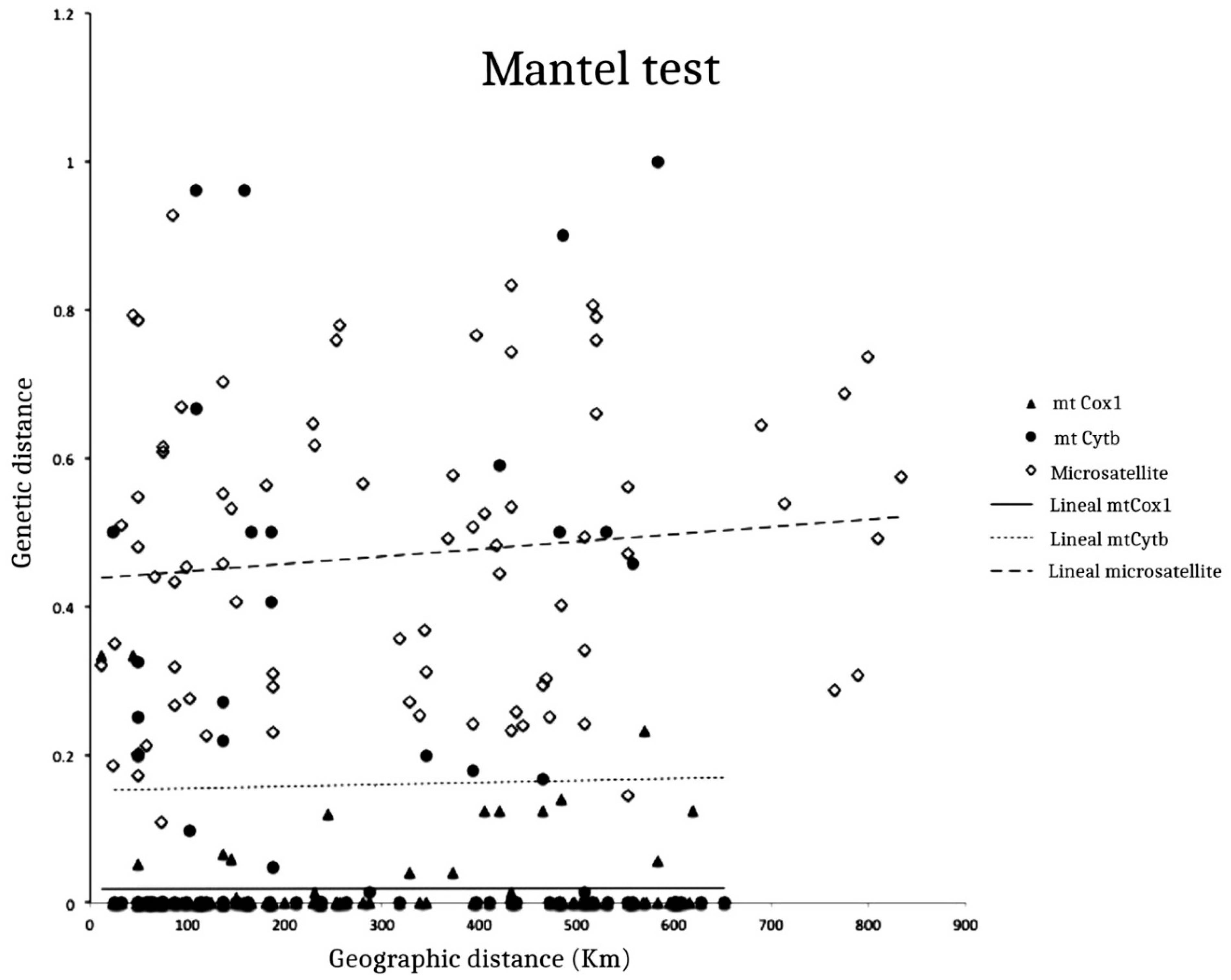
2.5. Isolation by Distance

To detect the effect of isolation by geographical distance (IBD), we compared the correlation of genetic distance (FST), RE = FST/(1 − FST) [57] with geographical distance [58]. The distances were obtained by following the channels of the rivers sampled with the measure tool of the ArcGIS program. IBD was estimated using the correlation coefficient (R2) for all pairs of populations for the 2 mitochondrial fragments and the 11 microsatellite loci with the Mantel test in the vegan package in RStudio [50].

3. Results

A fragment of 574 bases of mtCox1 (n = 72) and a fragment of 454 bases of mtCytb (n = 34) were obtained from three zones within the Usumacinta basin. In the dataset for the mtCox1 fragment, we recovered eight haplotypes with a total of seven variable sites, with a low haplotypic diversity of Hd = 0.281 and a low nucleotide diversity with a π value of 0.0006 (Table 1). The haplotype network for mtCox1 showed a star-like shape (Figure 2A), with Hap3 showing the highest frequency and being present at the 80% the sampled zones (Figure 2B). Despite this, the results indicated the presence of exclusive haplotypes for each zone: rainforest, Hap 1; floodplain, Hap 4, 5 and 6; river delta, Hap 7 and 8.
For the mtCytb fragment, four haplotypes were identified with two variable sites, with a relatively larger haplotype diversity (Hd = 0.615) but with a low π value of 0.001 (Table 1). In the mtCytb haplotype network, we observed that the four haplotypes were distributed more homogeneously among the sampled populations, with two haplotypes present in all the sampled localities (Figure 2B), while the other two haplotypes were only present in the FZ (that is, Jonuta, Emiliano Zapata and Catazaja). For both mitochondrial markers, the highest number of private haplotypes was found in the FZ (Table 1), which also showed the highest genetic diversity; thus, for mtCytb, the genetic diversity was Hd = 0.822 and for mtCox1, Hd = 0.36, while the lowest diversity was observed for the RZ: Hd = 0.46 and 0.32 for mtCytb and mtCox1, respectively.
In the hierarchical AMOVA for mtCox1 and mtCytb, most of the variation was recovered within populations: 86.61% and 92.99%, respectively (Table 2), with very low but not significant ΦCT values among groups (i.e., mtCox1 ΦCT = −0.032; mtCytb ΦCT = 0.061). Similarly, the differences between populations within groups were low but not significant (i.e., mtCox1 ΦSC = −0.080; mtCytb ΦSC = 0.009; mtCox1 ΦST = −0.044; mtCytb ΦST = 0.07 (Table 2)).

3.1. Microsatellite Structure

The Cun-22 and Cun-09 loci were excluded from the analysis because the Cun-22 locus showed more than 51% missing data, while the Cun-09 and Cun-10 loci were linked; therefore, we kept Cun-10, since it was the marker with least missing data (see Supplementary Material S1, Table S4: Linkage disequilibrium results of nine microsatellites from Centropomus undecimalis). The summary statistics for all microsatellite loci are presented in Table 1. The number of alleles per locus ranged from 6 to 21. Five loci exhibited departure from Hardy–Weinberg equilibrium (HWE), due, in some cases, to a statistically significant deficit of heterozygotes.
We found evidence that null alleles may be present at five loci (Cun-20, Cun-10-A, Cun-02, Cun-01 and Cun-06) but we found no evidence for allele dropout or stuttering during PCR amplification. We found no evidence of scoring error, no large allele dropout and no null alleles at the Cun-21-A, Cun-04-A, Cun-21-B and Cun-14 loci. In general, the number of private alleles was low across the sampling sites (Table 3), with four private alleles being found at Chajul, Lacantun and Canitzan.
A very small amount of genetic differentiation was detected among the Centropomus undecimalis populations studied, as revealed by significant pairwise FST values for 12 pairwise comparisons out of 77 (Table 4). A geographical pattern of the distribution of these differences was not recognized, but it could be identified that most of the significant differences were between the RD and the FZ.
Bayesian clustering via Evanno’s method (i.e., STRUCTURE) [46] indicated that the most likely number of clusters was K = 2 (Supplementary Material S2: Plots generated in STRUCTURE Harvester and DAPC). The first cluster included Tzendales, Canitzan, most of the individuals from Chacamax River and some individuals from the Lacantun River and San Pedro River (Figure 3A, individuals in green), suggesting a genetic differentiation of the populations from the RZ and FZ, while the second cluster included a mixture of individuals from the RD and some individuals from the RZ and FZ (Figure 3A, individuals in red).
Figure 3B shows the grouping obtained by STRUCTURE through Evanno′s test considering three genetic clusters (K = 3). One of the clusters included all individuals from the RD zone, some individuals from the RZ (some individuals from Lacantun River) and from the FZ (some individuals from Emiliano Zapata, San Pedro River and Chacamax) (individuals in red). A second cluster joined some individuals from the RZ (Tzendales River and Lacantun River) and from the FZ (Chacamax River, San Pedro River and Canitzan Lagoon) (individuals in green). The remaining cluster was a mixture of populations from the RZ and FZ.
After we removed the missing data, the microsatellite data matrix used for the analysis of the population structure via the DAPC analysis had 64 individuals. The first analysis in the DAPC considered two genetic clusters (K = 2), corresponding to the groups obtained with STRUCTURE through Evanno′s test (see Supplementary Material S3A: Discriminant analysis of principal components (DAPC): scatterplots of the discriminant analysis of principal components of the microsatellite data for three zones) and, after a cross-validation test, retained 10 principal components (PCs) with an accumulated variance of 60.1% for the total data. As can be observed in the graph, only a small number of individuals were grouped in the second cluster, which corresponded to a mixture of populations from the RZ and FZ.
In the DAPC, we considered the three genetic clusters (K = 3), obtained by STRUCTURE through Evanno′s test (see Supplementary Material S3B). Thus, in the discriminant analysis of principal components (DAPC), the scatterplots retained five principal components (PCs) with an accumulative variance of 39.5% for the total data, after a cross-validation test. Thus, one of the three clusters included all individuals from the RD zone, some individuals from the RZ (Lacantun River) and from the FZ (Canitzan Lagoon and San Pedro River). A second cluster joined individuals from the RZ (Tzendales River) and from the FZ (Chacamax River and Canitzan Lagoon). The third cluster grouped a mixture of populations from the RZ and FZ.
Finally, the find.clusters algorithm retrieved three different genetic clusters of the 13 populations of C. undecimalis analyzed, for all the runs performed (i.e., 10), showing the lowest BIC value (i.e., 79). For K = 3, the cross-validation test resulted in the retention of five principal components (PCs) with an accumulative variance of 39.5% for the total data. In this case, the three clusters were mostly the same as the ones previously described for the STRUCTURE software, with the only difference that in the third cluster, an individual from the RD zone was included. The scatterplot of individuals on the two main components of DAPC showed that they formed three groups, and no overlapping between the a priori defined groups (Figure 3C). We did not find evidence of substructuring among the clusters analyzed. In the hierarchical AMOVA, low but significant values of differentiation were recovered (Table 2). Most of the genetic variance was observed within the populations (94.04% by zones and 89.57% by STRUCTURE with K = 3). The differentiation among groups was low (FST = 0.059 by zones), as was that among populations within groups (FSC = 0.043); both differences were significant. We estimated the migration rate (m) using BayesASS as an indicator of gene flow among the genetic groups. The BayesASS average results using the groupings obtained with DAPC analysis (K = 3) and STRUCTURE software (K = 2 and K = 3) are shown in Supplementary Material S1, Table S5 (BayesASS results showing the average migration rate (mprom) by cluster obtained); for more information, see Supplementary Material S1, Table S6 (Results of 10 runs of the BayesASS algorithm, with the average and total number of times the results were achieved). In general, the m-values were low among the genetic clusters. The m-value from k = 1 to k = 2 was the lowest (DAPC = 0.009 and STRUCTURE = 0.008). The values of the product of m and Ne, which represents the number of migrating individuals, are shown in Table 5.

3.2. Isolation by Distance

Although we observed differences in the level of genetic diversity across the designated zones (RZ, FZ and RD), we did not find a correlation between the geographic and genetic distances for either mitochondrial marker (R2 = 0.005; p = 0.4265 and R2 = 0.0478; p = 0.3916 for mtCox1 and mtCytb, respectively) nor the nuclear loci (Figure 4, R2 = 0.1143, p = 0.1668).

4. Discussion

The Usumacinta River basin is one of the largest basins in the Gulf of Mexico, whose biological diversity is outstanding for the Mesoamerican region [29,59], with more than 170 species, including 50 fish families, making it one of the most diverse river basins in Mexico [20]. Its hydrological connectivity allows the common snook to complete its life cycle. The species is one of the most abundant, largest and most economically important, with a high commercial value, which has led to overfishing of the species, threatening their populations [60,61,62]. Testing the genetic structure of an euryhaline species such as the common snook provides a unique opportunity to demonstrate the importance of the hydrological connectivity of the Usumacinta River basin, providing a better understanding of its conservation status.

4.1. mtDNA Genetic Structure

Our mtDNA results in the common snook support a degree of connectivity among the three zones in the Usumacinta River basin, a pattern expected due to the migratory nature of the species, as well as previous observations of some of its populations in a smaller geographic area [25]. The star-like haplotype network is consistent with a lack of geographical structure, showing haplotypes with low levels of sequence divergence and a high frequency of singletons. A similar pattern can be related to rapid population expansion or selection, which caused the rapid spread of a mitochondrial lineage [63]. Despite the lack of a clear geographic differentiation, haplotype frequencies and exclusive haplotypes differ among the zones analyzed. Particularly, with the mtCox1 marker, we identified differences in haplotype occurrence and their frequencies between the rainforest and delta zones (the upper and lower parts of the basin, respectively). These results are consistent with previous comparative phylogeographic analyses of the basin, which considered endemic species data and phylogeographic analyses for a selected group of organisms (mainly cichlids and poecilids), and report differences between the upper and lower parts of the Usumacinta River basin [29]. These results provide additional evidence that could indicate the existence of geographic structure for some of the freshwater fauna in the basin (e.g., Centropomus undecimalis) and support the hypothesis that the Usumacinta does not correspond to a single biogeographic unit [29].
The floodplain was recovered as the most diverse zone (see Table 1), showing a higher number of exclusive haplotypes (i.e., Hap 4, 5 and 6 for Cox1 and Hap3 and 4 for Cytb, Figure 2A,B). Thus, the mtDNA variations suggested that the floodplain acts as a confluence zone between the rainforest and river delta zones for the common snook. This pattern of genetic transition was previously reported in the Astyanax aeneus species complex on the basis of mitochondrial markers [10], where the floodplain zone was also found to be a transition zone between the rainforest and delta zones of the Usumacinta River drainage.
Despite the aforementioned differences, we did not recover significant differences among zones according to the hierarchical AMOVA, suggesting that the levels of differentiation were fairly low among the zones. However, the molecular phylogeographic patterns gave additional evidence about the relevance of using barcodes as valuable tools to characterize and reveal cryptic diversity in widely distributed fish species. In accordance, the geographic structure found inside the basin shows the utility of genetic information for characterizing the diversity patterns in a region previously considered to be a single unit [13].

4.2. nucDNA Genetic Structure

Microsatellite loci showed low but significant levels of differentiation among the zones tested in this study. The heterozygote deficiency represents a deviation from the Hardy–Weinberg Equilibrium (HWE) when the observed heterozygosity (Ho) is less than the expected heterozygosity (He) [64]. These deviations from the HWE proportions can be generated by the presence of null alleles and by an irregular system of inbreeding or by population structure [64,65]. In our study, the heterozygote deficiency observed could be explained by the presence of null alleles in some loci, but they were not shared across populations. When we considered K = 2, one of the clusters was distributed in the rainforest and floodplain zones, which included individuals from the populations from Tzendales, Lacantun, Chacamax, San Pedro and Canitzan. The second group included a cluster that shows a wider distribution across the basin, from the delta to the rainforest zones (Figure 3). These results support the confluence of two different genotypic clusters of the common snook in the Usumacinta River basin, one of which was widely distributed in the lower part of the basin (the delta zone) and reached the uplands (the rainforest zone), while the second cluster, which showed a more restricted distribution, occurred in the rainforest and floodplain zones, possibly extending to the upper part of the Usumacinta basin in Guatemala. A similar pattern was previously reported in the white turtle (Dermatemys mawii) [26,27,28], in which two genetic clusters were recovered along the Usumacinta River basin.
The DAPC results suggest a high probability for K = 3. One of these genetic clusters is widely distributed across the Usumacinta basin and is dominant in the delta zone. Additionally, the rainforest and floodplain zones contain two different genotypic clusters; the first one coincides with the cluster detected for the K = 2 analysis and the second one is distributed among the remaining individuals from both zones, hierarchically dividing the upper (rainforest and floodplain) from the lower part of the basin (delta zone).
The ocurrence of different genetic clusters occurring in the upper Usumacinta (rainforest and floodplain zones) but not detected in the lower Usumacinta cluster (delta zone) is in agreement with a previous study which supported the existence of two biogeographic units within the Usumacinta River basin [29]. This biogeographic pattern could be the result of both recent and historical events influencing fish diversification in the basin [29]. Further studies including adjacent areas on the distribution of the common snook would allow a better understanding of the extent of the genetic clusters found here.
Additionally, the presence of two different genetic clusters in the upper part of the Usumacinta basin could be related to the occurrence of different migratory contingencies in the common snook populations. Previous studies on catadromous fish have shown that they can present alternative migratory tactics within a conditional strategy [66]; in this case, the individuals could make migratory decisions depending on the following factors: individual status (e.g., body condition, growth rate), interactions with other organisms and environmental conditions (e.g., habitat availability or river flow). Previous studies have shown a high environmental similarity between the delta and the floodplain zones, the latter being considered as a reservoir for diversity where fish species can reproduce [20,67,68]. Additionally, the common snook individuals collected from the floodplain zone presented advanced stages of gonadal development [17]. The fact that the two genetic clusters from the rainforest and floodplain were not present in the delta zone could reflect an alternative migratory contingence, in which the floodplain zone could provide the environmental conditions necessary for the common snook to complete their life cycle, as happens with other migratory species [68]. Further studies exploring the existence of migratory contingents in the life cycle of C. undecimalis based on otolith 87Sr/86Sr analysis could shed light about the variation in life cycles among individuals.

4.3. Gene Flow and Isolation by Distance

In this work, it was found that the migration rates for the three structuring models showed a low genetic flow between the estimated clusters (Figure 3), with a low number of possible migrants among them (Table 5). These low migration rates can promote differential segregation between genetic clusters, supporting the idea that these groups are well-discriminated units. However, in accordance with our previous results, neither type of examined markers (mtDNA and nucDNA) showed an isolation by distance (IBD) pattern, suggesting a more complex genetic structure in the C. undecimalis populations.
In this regard, the IBD, mitochondrial haplotypes and nuclear results are in agreement with a previous study by Hernández-Vidal et al. [25], in which the lack of an IBD pattern was described. However, in that study, the authors only compared two marine populations (referred to as the sea population here) vs. individuals from the San Pedro River near the Guatemala border, for a total of 79 individuals. Their results showed a 2% variance between the sea and the San Pedro River basin (in the floodplain zone), very similar to our results for those groups (nucDNA = 2.1%, mtCox1 = 3.29% and mtCytb = 6.13%; Table 2).
Based on the BayesASS results, we found a low gene flow among the genetic clusters recovered. However, since one of the genetic clusters recovered was found throughout the Usumacinta River basin, the structuring pattern related to geographic distance was not observed. In this regard, a previous study involving allozymes in C. undecimalis recovered strong differentiation between the Gulf of Mexico waters and the Caribbean populations, suggesting that these populations could correspond to different management units [18]. Additionally, recent studies of C. undecimalis, from the Gulf of Mexico to Brazil, showed very high genetic differentiation associated with the geographical distance between the populations [69,70]. The results for genetic structuring and the estimation of migration rates suggest that two to three different populations of the common snook converge in the Usumacinta River basin.
Hydrological connectivity, together with historical processes, could have played a major role in the genetic structure of the common snook population in the Usumacinta basin over different temporal and geographical scales [26,27,28]. Further studies including wider geographical sampling in the Gulf of Mexico and the Caribbean could help us to test these differential patterns of connectivity and genetic structure within the common snook across different regions.

4.4. Implications for Species Conservation

Our results could have important implications for species conservation and management. First, it is clear that the common snook migrates and disperses throughout the basin, from the rainforest zone in Mexico (Tzendales River and Lacantun River) and its border with Guatemala to the river delta zone. Thus, river connectivity is essential to allow the species to maintain its life cycle. On the other hand, the genetic differences found in the common snook, for which the floodplain zone was identified as the most diverse zone according to both mitochondrial and nuclear data, suggesting that this zone corresponds to a confluence between the rainforest and river delta zones in the Usumacinta River basin; thus, the floodplain zone corresponds to a relevant unit for the conservation and management of the species. In particular, the San Pedro River represents a unique region, due to the environmental conditions, which could provide particular biological dynamics that allow the species to reproduce. Thus, future studies could shed more light in this regard [71]. Alterations in river connectivity will impact the life history of the common snook, including its migratory and dispersal behavior and population size contractions, affecting the fisheries in the region and ultimately species conservation. The identification of the high-diversity unit zones (i.e., the FZ) through the use of barcodes could favor the implementation of a responsible management program in these zones by decision-makers for preserving not only the species but also its genetic diversity.
Regarding the genetic cluster recovered with the nuclear markers, we suggest that these could represent alternative reproductive stocks of the species within the Usumacinta basin; thus, even though we did not recover a geographic structure, we consider that the basin represents a very important system for the conservation of the species’ genetic diversity, where alternative reproductive strategies could have been taking place.
Finally, our study also recovered the diversity information of mitochondrial and nuclear data that in contrast with previous studies that also shed light on the current status of the species. With the two mitochondrial markers, the genetic diversity recovered was lower (i.e., mtCox1 Hd = 0.28 and mtCytb Hd = 0.62) than previously reported for the species [18,72], and also in comparison with other euryhaline species [73,74]; for mtCox1, Hap3 was present in 80% of the samples analyzed. Similarly, in the nuclear data, the heterozygosity values obtained in our study were lower than those previously reported for 5 of our 11 microsatellite loci [25]. This information could be explained by our sample size; however, the two types of data provide evidence that is consistent with biogeographic patterns. Moreover, our results could also be related to an overexploitation of the species by the local fisheries, urging the local authorities to implement conservation and management programs to preserve the species’ evolutionary history.

Supplementary Materials

The following are available online at https://0-www-mdpi-com.brum.beds.ac.uk/article/10.3390/d13080347/s1. Supplementary Material S1: Table S1: Sampling localities from the Usumacinta River basin. Table S2: Eleven microsatellite loci used in determining genetic variation among the Centropomus undecimalis samples from 13 sampling localities along the Usumacinta River basin. Table S3: Genotyping of nine loci of Centropomus undecimalis. Table S4: Linkage disequilibrium results of nine microsatellites from Centropomus undecimalis. Table S5: BayesASS results showing the average migration rate (mprom) by cluster, obtained with DAPC (k = 3) and STRUCTURE (k = 2, k = 3). SD, standard deviation; CI, 95% confidence interval; N, the number of times this outcome was reached over 10 runs with varying starting seeds. Table S6: Results of 10 runs of the BayesASS algorithm, with the average and total number of times the results were achieved. Supplementary Material S2. Plots generated in STRUCTURE Harvester and DAPC. (A) The mean log likelihood of the data [L(K)]. (B) Estimation of population clustering levels from seven microsatellite genotypes following Evanno′s test [46]. (C) BIC value changes (find.clusters function) of DAPC. Supplementary Material S3. Discriminant analysis of principal components (DAPC): scatterplots of the discriminant analysis of principal components of the microsatellite data for three zones.

Author Contributions

Conceptualization: J.T.-M., C.P.O.-G. and R.R.-H.; Methodology: J.T.-M., C.P.O.-G. and M.A.A.G.-S.; Formal analysis: J.T.-M., C.P.O.-G. and M.A.A.G.-S.; Writing—original draft preparation: J.T.-M. and C.P.O.-G.; Writing—review and editing: C.P.O.-G., R.R.-H. and M.A.A.G.-S.; Visualization: C.P.O.-G. and R.R.-H.; Resources: C.P.O.-G. and R.R.-H.; Funding acquisition: C.P.O.-G. and R.R.-H. All authors have read and agreed to the published version of the manuscript.

Funding

This research was support from PAPIIT, UNAM, Project number IN212419 and the project “Conectividad y Diversidad Funcional de la Cuenca del Río Usumacinta” (FID-ECOSUR 784-1004).

Institutional Review Board Statement

Field collection permit and protocols related to the animal care ethics was approved by the Secretaria del Medio Ambiente y Recursos Naturales (SEMARNAT: PPF/DGOPA-249/14).

Informed Consent Statement

Not applicable.

Data Availability Statement

The data of the sequences used will be available at https://0-www-ncbi-nlm-nih-gov.brum.beds.ac.uk/genbank/.

Acknowledgments

We thank Posgrado de El Colegio de la Frontera Sur for the support given to Jazmín Terán-Martínez during her PhD study. We thank Miriam Soria-Barreto and Alfonso Gonzalez-Díaz for their comments and suggestions on the study. We also thank Alberto Macossay-Cortéz, Abraham Aragón-Flores and Mayra Contreras-Flores for help with collecting fish during field trips; Cesar Maya-Bernal and Cinthya Mendoza for their support in the laboratory; and Pablo Sandoval-Rivera for his contribution to the elaboration of the cartographic content. Jazmín Terán-Martínez was funded by Consejo Nacional de Ciencia y Tecnología, Mexico (CONACyT), scholarship number 562922. SEMARNAT Fishing permit No. PPF/DGOPA-249/14.

Conflicts of Interest

The authors declare no conflict of interest. The funders had no role in the design of the study; in the collection, analyses, or interpretation of data; in the writing of the manuscript; or in the decision to publish the results.

References

  1. Pringle, C.M.; Freeman, M.C.; Freeman, B.J. Regional Effects of Hydrologic Alterations on Riverine Macrobiota in the New World: Tropical–Temperate Comparisons. BioScience 2000, 50, 807–823. [Google Scholar] [CrossRef] [Green Version]
  2. Pringle, C. What Is Hydrologic Connectivity and Why Is It Ecologically Important? Hydrological Process: Hoboken, NJ, USA, 2003; Volume 17, pp. 2685–2689. [Google Scholar]
  3. Calles, O.; Greenberg, L. Connectivity is a two-way street-the need for a holistic approach to fish passage problems in regulated rivers. River Res. Appl. 2009, 25, 1268–1286. [Google Scholar] [CrossRef]
  4. Ward, J.V. The Four-Dimensional Nature of Lotic Ecosystems. J. N. Am. Benthol. Soc. 1989, 8, 2–8. [Google Scholar] [CrossRef]
  5. Branco, P.; Segurado, P.; Santos, J.; Pinheiro, P.; Ferreira, M. Does longitudinal connectivity loss affect the distribution of freshwater fish? Ecol. Eng. 2012, 48, 70–78. [Google Scholar] [CrossRef]
  6. Lucas, M.C.; Baras, E. Migration of Freshwater Fishes; Lucas, M., Baras, E., Thom, T., Duncan, A., Slavík, O., Eds.; Blackwell Science: Maden, MA, USA, 2001. [Google Scholar]
  7. Yi, Y.; Yang, Z.; Zhang, S. Ecological influence of dam construction and river-lake connectivity on migration fish habitat in the Yangtze River basin, China. Procedia Environ. Sci. 2010, 2, 1942–1954. [Google Scholar] [CrossRef] [Green Version]
  8. Collins, S.M.; Bickford, N.; McIntyre, P.B.; Coulon, A.; Ulseth, A.J.; Taphorn, D.C.; Flecker, A.S. Population Structure of a Neotropical Migratory Fish: Contrasting Perspectives from Genetics and Otolith Microchemistry. Trans. Am. Fish. Soc. 2013, 142, 1192–1201. [Google Scholar] [CrossRef]
  9. Hand, B.K.; Lowe, W.H.; Kovach, R.P.; Muhlfeld, C.C.; Luikart, G. Landscape community genomics: Understanding eco-evolutionary processes in complex environments. Trends Ecol. Evol. 2015, 30, 161–168. [Google Scholar] [CrossRef]
  10. Garcia, C.P.O.; De Biología, U.I.; Bernal, C.F.M.; Hernández, R.R.; Biomédicas, U.I.D.I. Ecosur Evaluación de la Diversidad de Linajes en Sistemas Dulceacuícolas tropicales (D-LSD): El Sistema Usumacinta como caso de estudio. In Antropización: Primer Análisis Integral; Universidad Nacional Autónoma de México, Centro de Investigaciones en Geografía Ambiental: Mexico City, Mexico, 2019; pp. 125–148. [Google Scholar]
  11. Oosthuizen, C.J.; Cowley, P.D.; Kyle, S.R.; Bloomer, P. High genetic connectivity among estuarine populations of the riverbream Acanthopagrus vagus along the southern African coast. Estuar. Coast. Shelf Sci. 2016, 183, 82–94. [Google Scholar] [CrossRef]
  12. Sork, V.L.; Smouse, P.E. Genetic analysis of landscape connectivity in tree populations. Landsc. Ecol. 2006, 21, 821–836. [Google Scholar] [CrossRef]
  13. DeSalle, R.; Goldstein, P. Review and Interpretation of Trends in DNA Barcoding. Front. Ecol. Evol. 2019, 7, 302. [Google Scholar] [CrossRef] [Green Version]
  14. Ornelas-García, C.P.; Domínguez-Domínguez, O.; Doadrio, I. Evolutionary history of the fish genus Astyanax Baird & Girard (1854) (Actinopterygii, Characidae) in Mesoamerica reveals multiple morphological homoplasies. BMC Evol. Biol. 2008, 8, 340. [Google Scholar] [CrossRef] [Green Version]
  15. Valdez-Moreno, M.; Ivanova, N.V.; Elías-Gutiérrez, M.; Pedersen, S.L.; Bessonov, K.; Hebert, P.D.N. Using eDNA to biomonitor the fish community in a tropical oligotrophic lake. PLoS ONE 2019, 14, e0215505. [Google Scholar] [CrossRef] [Green Version]
  16. Frankham, R. Stress and adaptation in conservation genetics. J. Evol. Biol. 2005, 18, 750–755. [Google Scholar] [CrossRef] [PubMed]
  17. Hernández-Vidal, U.; Chiappa-carrara, X.; Contreras-Sánchez, W.M. Reproductive variability of the common snook, Centropomus undecimalis, in environments of contrasting salinities interconnected by the Grijalva–Usumacinta fluvial system. Cienc. Mar. 2014, 40, 173–185. [Google Scholar] [CrossRef] [Green Version]
  18. Tringali, M.; Bert, T. The genetic stock structure of common snook (Centropomus undecimalis). Can. J. Fish. Aquat. Sci. 1996, 53, 974–984. [Google Scholar] [CrossRef]
  19. Mendonça, J.T.; Chao, L.; Albieri, R.J.; Giarrizzo, T.; da Silva, F.M.S.; Castro, M.G.; Brick-Peres, M.; Villwock de Miranda, L.; Vieira, J.P. Centropomus undecimalis. The IUCN Red List of Threatened Species 2019: E.T191835A82665184. 2019. Available online: https://0-dx-doi-org.brum.beds.ac.uk/10.2305/IUCN.UK.2019-2.RLTS.T191835A82665184.en (accessed on 30 May 2021).
  20. Soria-Barreto, M.; González-Díaz, A.A.; Castillo-Domínguez, A.; Álvarez-Pliego, N.; Rodiles-Hernández, R. Diversity of fish fauna in the Usumacinta Basin, Mexico. Rev. Mex. Biodivers. 2018, 89, 100–117. [Google Scholar]
  21. Garcia, M.A.P.; Mendoza-Carranza, M.; Contreras-Sánchez, W.; Ferrara, A.; Huerta-Ortiz, M.; Gómez, R.E.H. Comparative age and growth of common snook Centropomus undecimalis (Pisces: Centropomidae) from coastal and riverine areas in Southern Mexico. Rev. Biol. Trop. 2013, 61, 807–819. [Google Scholar] [CrossRef] [Green Version]
  22. Castro-Aguirre, J.L.; Espinosa-Pérez, H.; Schmitter-Soto, J.J. Ictiofauna Estuarino-Lagunar y Vicaria de México; Editorial Limusa: La Paz, Baja California Sur, Mexico, 1999; ISBN 9681857747. [Google Scholar]
  23. Adams, A.J.; Wolfe, R.K.; Layman, C.A. Preliminary Examination of How Human-driven Freshwater Flow Alteration Affects Trophic Ecology of Juvenile Snook (Centropomus undecimalis) in Estuarine Creeks. Chesap. Sci. 2009, 32, 819–828. [Google Scholar] [CrossRef]
  24. Miller, R.R. Peces dulceacuícolas de México; CONABIO, SIMAC, ECOSUR, Desert Fishes of Council: Mexico City, Mexico, 2009. [Google Scholar]
  25. Hernández-Vidal, U.; Lesher-Gordillo, J.; Contreras-Sánchez, W.M.; Chiappa-Carrara, X. Variabilidad genética del robalo común Centropomus undecimalis (Perciformes: Centropomidae) en ambiente marino y ribereño interconectados. Rev. Biol. Trop. 2014, 62, 627–636. [Google Scholar] [CrossRef] [Green Version]
  26. González-Porter, G.P.; Hailer, F.; Flores-Villela, O.; García-Anleu, R.; Maldonado, J.E. Patterns of genetic diversity in the critically endangered Central American river turtle: Human influence since the Mayan age? Conserv. Genet. 2011, 12, 1229–1242. [Google Scholar] [CrossRef]
  27. Gonzalez-Porter, G.P.; Maldonado, J.E.; Flores-Villela, O.; Vogt, R.C.; Janke, A.; Fleischer, R.C.; Hailer, F. Cryptic Population Structuring and the Role of the Isthmus of Tehuantepec as a Gene Flow Barrier in the Critically Endangered Central American River Turtle. PLoS ONE 2013, 8, e71668. [Google Scholar] [CrossRef] [Green Version]
  28. Martínez-Gómez, J. Sistemática Molecular e Historia Evolutiva de la Familia Dermatemydidae; Universidad de Ciencias y Artes de Chiapas: Tuxtla Gutiérrez, Chiapas, Mexico, 2017. [Google Scholar]
  29. Elías, D.J.; Mcmahan, C.D.; Matamoros, W.A.; Gómez-González, A.E.; Piller, K.R.; Chakrabarty, P. Scale(s) matter: Deconstructing an area of endemism for Middle American freshwater fishes. J. Biogeogr. 2020, 47, 2483–2501. [Google Scholar] [CrossRef]
  30. Sonnenberg, R.; Nolte, A.W.; Tautz, D. An evaluation of LSU rDNA D1-D2 sequences for their use in species identification. Front. Zoöl. 2007, 4, 6. [Google Scholar] [CrossRef] [Green Version]
  31. Ward, R.D.; Zemlak, T.S.; Innes, B.H.; Last, P.R.; Hebert, P.D. DNA barcoding Australia’s fish species. Philos. Trans. R. Soc. B Biol. Sci. 2005, 360, 1847–1857. [Google Scholar] [CrossRef] [PubMed]
  32. Zardoya, R.; Doadrio, I. Phylogenetic relationships of Iberian cyprinids: Systematic and biogeographical implications. Proc. R. Soc. B Boil. Sci. 1998, 265, 1365–1372. [Google Scholar] [CrossRef] [PubMed] [Green Version]
  33. Seyoum, S.; Tringali, M.D.; Sullivan, J.G. Isolation and characterization of 27 polymorphic microsatellite loci for the common snook, Centropomus undecimalis. Mol. Ecol. Notes 2005, 5, 924–927. [Google Scholar] [CrossRef]
  34. Hall, T.A. BioEdit: A User-Friendly Biological Sequence Alignment Editor and Analysis Program for Windows 95/98/NT. Nucleic Acids Symp. Series 1999, 41, 95–98. [Google Scholar]
  35. Rozas, J.; Ferrer-Mata, A.; Sánchez-DelBarrio, J.C.; Guirao-Rico, S.; Librado, P.; Ramos-Onsins, S.E.; Sánchez-Gracia, A. DnaSP 6: DNA Sequence Polymorphism Analysis of Large Data Sets. Mol. Biol. Evol. 2017, 34, 3299–3302. [Google Scholar] [CrossRef] [PubMed]
  36. Leigh, J.W.; Bryant, D. Popart: Full-feature software for haplotype network construction. Methods Ecol. Evol. 2015, 6, 1110–1116. [Google Scholar] [CrossRef]
  37. Stamatakis, A. RAxML version 8: A tool for phylogenetic analysis and post-analysis of large phylogenies. Bioinformatics 2014, 30, 1312–1313. [Google Scholar] [CrossRef]
  38. Miller, M.A.; Pfeiffer, W.; Schwartz, T. Creating the CIPRES Science Gateway for inference of large phylogenetic trees. Gatew. Comput. Environ. Workshop (GCE) 2010, 1–8. [Google Scholar] [CrossRef] [Green Version]
  39. Darriba, D.; Taboada, G.L.; Doallo, R.; Posada, D. jModelTest 2: More models, new heuristics and parallel computing. Nat. Methods 2012, 9, 772. [Google Scholar] [CrossRef] [Green Version]
  40. Excoffier, L.; Lischer, H.E.L. Arlequin suite ver 3.5: A new series of programs to perform population genetics analyses under Linux and Windows. Mol. Ecol. Resour. 2010, 10, 564–567. [Google Scholar] [CrossRef]
  41. Van Oosterhout, C.; Hutchinson, W.F.; Wills, D.P.M.; Shipley, P. micro-checker: Software for identifying and correcting genotyping errors in microsatellite data. Mol. Ecol. Notes 2004, 4, 535–538. [Google Scholar] [CrossRef]
  42. Raymond, M.; Rousset, F. GENEPOP (Version 1.2): Population Genetics Software for Exact Tests and Ecumenicism. J. Hered. 1995, 86, 248–249. [Google Scholar] [CrossRef]
  43. Peakall, R.; Smouse, P.E. Genalex 6: Genetic analysis in Excel. Population genetic software for teaching and research. Mol. Ecol. Notes 2006, 6, 288–295. [Google Scholar] [CrossRef]
  44. Weir, B.S.; Cockerham, C.C. Estimating F-Statistics for the Analysis of Population Structure. Evolution 1984, 38, 1358. [Google Scholar] [CrossRef] [PubMed]
  45. Pritchard, J.K.; Stephens, M.; Donnelly, P. Inference of population structure using multilocus genotype data. Genetics 2000, 155, 945–959. [Google Scholar] [CrossRef] [PubMed]
  46. Evanno, G.; Regnaut, S.; Goudet, J. Detecting the number of clusters of individuals using the software structure: A simulation study. Mol. Ecol. 2005, 14, 2611–2620. [Google Scholar] [CrossRef] [Green Version]
  47. Earl, D.A.; Vonholdt, B.M. STRUCTURE HARVESTER: A website and program for visualizing STRUCTURE output and implementing the Evanno method. Conserv. Genet. Resour. 2011, 4, 359–361. [Google Scholar] [CrossRef]
  48. Jombart, T.; Devillard, S.; Balloux, F. Discriminant analysis of principal components: A new method for the analysis of genetically structured populations. BMC Genet. 2010, 11, 94. [Google Scholar] [CrossRef] [Green Version]
  49. Jombart, T.; Ahmed, I. adegenet 1.3-1: New tools for the analysis of genome-wide SNP data. Bioinformatics 2011, 27, 3070–3071. [Google Scholar] [CrossRef] [Green Version]
  50. Team, R. A Language and Environment for Statistical Computing; R Core Team: Vienna, Austria, 2006. [Google Scholar]
  51. Jombart, T.; Collins, C. A Tutorial for Discriminant Analysis of Principal Components (DAPC) Using Adegenet 2.0.0; Imperial College London, MRC Centre for Outbreak Analysis and Modelling: London, UK, 2015. [Google Scholar]
  52. Criscuolo, N.G.; Angelini, C. StructuRly: A novel shiny app to produce comprehensive, detailed and interactive plots for population genetic analysis. PLoS ONE 2020, 15, e0229330. [Google Scholar] [CrossRef] [PubMed] [Green Version]
  53. Kamvar, Z.N.; Tabima, J.F.; Grünwald, N.J. Poppr: An R package for genetic analysis of populations with clonal, partially clonal, and/or sexual reproduction. PeerJ 2014, 2, e281. [Google Scholar] [CrossRef] [Green Version]
  54. Wilson, G.A.; Rannala, B. Bayesian Inference of Recent Migration Rates Using Multilocus Genotypes. Genetics 2003, 163, 1177–1191. [Google Scholar] [CrossRef] [PubMed]
  55. Do, C.; Waples, R.S.; Peel, D.; Macbeth, G.M.; Tillett, B.J.; Ovenden, J.R. NeEstimatorv2: Re-implementation of software for the estimation of contemporary effective population size (Ne) from genetic data. Mol. Ecol. Resour. 2013, 14, 209–214. [Google Scholar] [CrossRef] [PubMed]
  56. Rohlf, F.J. Comparative methods for the analysis of continuous variables: Geometric interpretations. Evolution 2001, 55, 2143–2160. [Google Scholar] [CrossRef] [PubMed]
  57. Slatkin, M. A measure of population subdivision based on microsatellite allele frequencies. Genetics 1995, 139, 457–462. [Google Scholar] [CrossRef]
  58. Wright, S. ISOLATION BY DISTANCE. Genetics 1943, 28, 114–138. [Google Scholar] [CrossRef]
  59. Yáñez-Arancibia, A.; Day, J.W.; Currie-Alder, B. Functioning of the Grijalva-Usumacinta River Delta, Mexico: Challenges for Coastal Management. Ocean Yearb. Online 2009, 23, 473–501. [Google Scholar] [CrossRef]
  60. Mendoza-Carranza, M.; Hoeinghaus, D.J.; Garcia, A.M.; Romero-Rodriguez, Á. Aquatic food webs in mangrove and seagrass habitats of Centla Wetland, a Biosphere Reserve in Southeastern Mexico. Neotrop. Ichthyol. 2010, 8, 171–178. [Google Scholar] [CrossRef] [Green Version]
  61. Barrientos, C.; Quintana, Y.; Elías, D.J.; Rodiles-Hernández, R. Peces nativos y pesca artesanal en la cuenca Usumacinta, Guatemala. Rev. Mex. Biodivers. 2018, 89, 118–130. [Google Scholar] [CrossRef] [Green Version]
  62. Barba-Macías, E.; Juárez-Flores, J.; Trinidad-Ocaña, C.; Sánchez-Martínez, A.D.J.; Mendoza-Carranza, M. Socio-ecological Approach of Two Fishery Resources in the Centla Wetland Biosphere Reserve. In Socio-Ecological Studies in Natural Protected Areas; Springer Science and Business Media LLC: Berlin, Germany, 2020; pp. 627–656. [Google Scholar]
  63. Mirol, P.M.; Routtu, J.; Hoikkala, A.; Butlin, R.K. Signals of demographic expansion in Drosophila virilis. BMC Evol. Biol. 2008, 8, 59. [Google Scholar] [CrossRef] [PubMed] [Green Version]
  64. Rousset, F.; Raymond, M. Testing heterozygote excess and deficiency. Genetics 1995, 140, 1413–1419. [Google Scholar] [CrossRef]
  65. De Meeûs, T. Revisiting FIS, FST, Wahlund effects, and null alleles. J. Hered. 2018, 109, 446–456. [Google Scholar] [CrossRef] [Green Version]
  66. Crook, D.A.; Buckle, D.J.; Allsop, Q.; Baldwin, W.; Saunders, T.M.; Kyne, P.M.; Woodhead, J.D.; Maas, R.; Roberts, B.; Douglas, M.M. Use of otolith chemistry and acoustic telemetry to elucidate migratory contingents in barramundi Lates calcarifer. Mar. Freshw. Res. 2017, 68, 1554. [Google Scholar] [CrossRef] [Green Version]
  67. Ochoa-Gaona, S.; Ramos-Ventura, L.J.; Moreno-Sandoval, F.; Jiménez-Pérez, N. del C.; Haas-Ek, M.A.; Muñiz-Delgado, L.E. Diversidad de flora acuática y ribereña en la cuenca del río Usumacinta, México. Rev. Mex. Biodivers. 2018, 89, 3–44. [Google Scholar]
  68. Vaca, R.A.; Golicher, D.J.; Rodiles-Hernández, R.; Castillo-Santiago, M. Ángel; Bejarano, M.; Navarrete-Gutiérrez, D.A. Drivers of deforestation in the basin of the Usumacinta River: Inference on process from pattern analysis using generalised additive models. PLoS ONE 2019, 14, e0222908. [Google Scholar] [CrossRef] [PubMed]
  69. Carvalho-Filho, A.; De Oliveira, J.; Soares, C.; Araripe, J. A new species of snook, Centropomus (Teleostei: Centropomidae), from northern South America, with notes on the geographic distribution of other species of the genus. Zootaxa 2019, 4671, 81–92. [Google Scholar] [CrossRef]
  70. De Oliveira, J.N.; Gomes, G.; Rêgo, P.S.D.; Moreira, S.; Sampaio, I.; Schneider, H.; Araripe, J. Molecular data indicate the presence of a novel species of Centropomus (Centropomidae–Perciformes) in the Western Atlantic. Mol. Phylogenet. Evol. 2014, 77, 275–280. [Google Scholar] [CrossRef]
  71. Castillo-Domínguez, A.; Barba Macías, E.; Navarrete, A. de J.; Rodiles-Hernández, R.; Jiménez Badillo, M. de L. Ictiofauna de los humedales del río San Pedro, Balancán, Tabasco, México. Rev. Biol. Trop. 2011, 59, 693–708. [Google Scholar] [PubMed]
  72. Anderson, J.; Williford, D.; González-Barnes, A.; Chapa, C.; Martinez-Andrade, F.; Overath, R.D. Demographic, Taxonomic, and Genetic Characterization of the Snook Species Complex ( Centropomus spp.) along the Leading Edge of Its Range in the Northwestern Gulf of Mexico. N. Am. J. Fish. Manag. 2020, 40, 190–208. [Google Scholar] [CrossRef]
  73. Rocha-Olivares, A.; Garber, N.M.; Stuck, K.C. High genetic diversity, large inter-oceanic divergence and historical demography of the striped mullet. J. Fish Biol. 2000, 57, 1134–1149. [Google Scholar] [CrossRef]
  74. Song, C.Y.; Sun, Z.C.; Gao, T.X.; Song, N. Structure Analysis of Mitochondrial DNA Control Region Sequences and its Applications for the Study of Population Genetic Diversity of Acanthogobius ommaturus. Russ. J. Mar. Biol. 2020, 46, 292–301. [Google Scholar] [CrossRef]
Figure 1. Map of the sampled localities for Centropomus undecimalis. Triangles correspond to the rainforest (RZ), squares correspond to the floodplain (FZ) and the circles correspond to the river delta (RD). Lagoons are represented by the shaded polygons.
Diversity 13 00347 g001
Figure 2. (A) ML haplotype networks for mtCox1 and mtCytb. The area of the circles is proportional to the number of sequences found for each haplotype. Partitions and colors inside the circles represent the proportion of each zone within each haplotype. (B) Frequencies and geographic distribution of mtCox1 and mtCytb haplotypes determined by combining allelic variants. The polygon indicates the distribution within the sampled area (rainforest, floodplain and river delta); n represents the number of sequences by haplotype.
Diversity 13 00347 g002
Figure 3. Assessment of population genetic structure by Bayesian cluster analysis and DAPC based on the microsatellite data. Bayesian Analysis was inferred at K = 2 based on locus data. Each single vertical line represents an individual and its proportional membership probability among the K clusters. (A) K = 2; (B) K = 3. (C) Scatterplots of the discriminant analysis of principal components of the microsatellite data, using find.clusters, for three zones. The axes represent the first two linear discriminants (LD). Each circle represents a cluster and each dot represents an individual.
Diversity 13 00347 g003
Figure 4. Mantel test. Correlation between genetic distance via Slatkin’s linearized method and the geographic distance (km), including the three markers (mtCox1, mtCytb and microsatellites). R2 = 0.005 (p = 0.4265) for mtCox1; R2 = 0.0478 (p = 0.3916) for mtCytb and R2 = 0.1143 (p = 0.1668) for microsatellites. The dotted line corresponds to the adjusted mtCytb data, the solid line corresponds to the mtCox1 data and dashed line corresponds to the adjusted microsatellite data.
Diversity 13 00347 g004
Table 1. Genetic diversity estimations of mtDNA for each zone of the common snook (Centropomus undecimalis): n = number of sequences; h = number of haplotypes; Hd = haplotypic diversity; S = number of variable sites; k = average pairwise nucleotide differences; π = nucleotide diversity. Summary statistics for nine polymorphic microsatellite loci: n = number of individuals with amplification; Na = number of alleles per locus; Ne = effective number of alleles per locus; HO = observed heterozygosity; He = expected heterozygosity; FIS = fixation index given for each locus. Values with the asterisk represent significant deviations from Hardy–Weinberg equilibrium.
mtDNALocus
Group mtCoxCyt-b Cun20Cun 10ACun 02Cun 21ACun 04ACun 01Cun 021BCun 06Cun 14
Rainforest zone
n = 23
n1710n202021221823222222
h32Na14.00015.0008.0005.0005.0008.0005.0007.00010.000
Hd0.3230.466Ne7.61911.4296.3001.7703.9273.3483.7964.9905.378
S21Ho0.9500.9000.5710.5000.8890.7390.8640.6360.864
k0.3380.001He0.8690.9130.8410.4350.7450.7010.7370.8000.814
π0.00050.466FIS−0.094 *0.0140.321−0.150−0.193−0.054−0.1730.204 *−0.061All locus FIS −0.011
Floodplain zone
n = 29
n2910n242729292327292629
h54Na15.00019.0008.0003.0006.00011.0006.0006.00010.000
Hd0.3690.822Ne6.77612.6786.5701.5973.7923.4553.1034.7116.029
S32Ho0.7080.8150.4480.4830.6960.5560.7240.5770.862
k0.4581.08He0.8520.9210.8480.3740.7360.7110.6780.7880.834
π0.00080.002FIS0.1690.1150.471 *−0.2910.0550.218 *−0.0680.268 *−0.033 *All locus
FIS 0.085
River delta
n = 29
n2614n292929292929292829
h32Na6.00017.0003.0003.0005.00011.0006.0004.00010.000
Hd0.1500.538Ne4.8907.4102.6831.2793.2662.4484.1021.7446.207
S31Ho0.6900.8620.5520.2410.6210.5860.7930.5710.759
k0.2300.538He0.7950.8650.6270.2180.6940.5920.7560.4270.839
π0.00040.001FIS0.1330.0030.120−0.1060.1050.009 *−0.049−0.3390.096All locus
FIS 0.011
Alln7234n737679807079807680
h84Na1821866146914
Hd0.2810.615Ne4.2165.9333.2501.5623.1542.9373.1112.3704.390
S72Ho0.7840.8680.4950.4100.7320.6520.7720.5680.822
k0.3540.722He0.7430.8150.6470.2760.6740.6350.6610.5270.756
π0.00060.001FIS0.071 0.0490.331 −0.203 −0.015 0.067−0.0970.1130.001
Table 2. Analysis of molecular variance (AMOVA) for two mitochondrial and nine microsatellite loci, among zones (rainforest, floodplain and river delta) and groups obtained with DAPC and STRUCTURE. Significant values are shown with the asterisk (p < 0.05).
MarkerVariance Among Groups (%)Variance among Populations within Groups (%)Variance
within Populations (%)
Among Groups
FCT/Φ CT
Among Populations
FSC/Φ SC
Within Populations
FST/Φ ST
mtCox13.2916.0086.610.03295−0.08010−0.04451
mtCytb6.130.8892.990.06134 0.009360.07013
Microsatellite
K = 3 DACP
11.11−0.6989.570.111 *−0.007 0.104 *
Microsatellite
K = 2 STRUCTURE
5.790103.1713891.030.05790.03360.089
K = 3 STRUCTURE1.694.2794.040.016 *0.043 *0.059 *
Table 3. Descriptive statistics for the microsatellite data in the Usumacinta River basin. Na = number of different alleles; Na (Freq ≥ 5%) = number of different alleles with a frequency ≥ 5%; Ne = number of effective alleles; Np = number of private alleles or the number of alleles unique to a single population.
PopulationNaNa Freq. ≥ 5%NeNp
Tzendales River3.5563.5563.1151
Lacantun River5.8895.8894.2364
Chajul5.1115.1114.0124
Benemerito3.6673.6672.8891
Emiliano Zapata4.3334.3333.4262
San Pedro River5.3335.3334.0821
Chacamax River3.7783.7783.1652
Jonuta4.0004.0003.4210
Canitzan Lagoon5.2225.2224.0164
Pom Lagoon5.1114.0003.4151
Palizada River4.5564.5563.1682
Terminos Lagoon3.0003.0002.4951
Sea4.5564.5563.2250
Table 4. Paired FST values among the 13 sampling localities of Centropomus undecimalis in the Usumacinta basin. Values with the asterisk represent significant values after Bonferroni correction.
TzendalesLacantun RiverChajulBenemeritoEmiliano ZapataSan Pedro RiverChacamaxJonutaCanitzanPom LagoonPalizada RiverTerminos LagoonSea
Tzendales0
Lacantun River0.0150
Chajul0.1170.0540
Benemerito0.0030.0340.0900
Emiliano Zapata0.0890.054−0.0130.0670
San Pedro
River
0.0200.0250.0880.085 *0.081 *0
Chacamax0.0930.0650.0630.104 *0.0640.0430
Jonuta0.0430.0140.0900.1320.107−0.0090.040
Canitzan0.0460.0270.0690.0780.082 *−0.0070.017−0.0040
Pom Lagoon0.1130.0820.0190.127−0.0660.1110.1120.1210.0970
Palizada River0.0410.00020.0150.091−0.004−0.0020.037−0.003−0.0010.0110
Terminos Lagoon0.0040.0250.101 *−0.0340.0640.088 *0.1150.0840.094 *0.104 *0.068 *0
Sea0.0510.0380.106−0.020.1020.1250.1030.1410.114 *0.148 *0.118 *−0.0380
Table 5. The estimated numbers of migrating individuals, calculated as the product of the average migration rate (m) and effective population size (Ne).
From k = 1From k = 2From k = 3Ne
DAPC
To K = 1(m = 0.9745)
86.9254
(m = 0.042)
3.7464
(m = 0.0244)
2.17648
89.2
To K = 2(m = 0.009)
0.0531
(m = 0.9159)
5.40381
(m = 0.0254)
0.14986
5.9
To K = 3(m = 0.0164)
0.19516
(m = 0.042)
0.4998
(m = 0.9501)
11.30619
11.9
STRUCTURE K = 3
To K = 1(m = 0.95581)
94.434028
(m = 0.07456)
7.366528
(m = 0.04342)
4.289896
98.8
To K = 2(m = 0.00872)
0.142136
(m = 0.88829)
14.479127
(m = 0.02753)
0.448739
16.3
To K = 3(m = 0.03545)
0.57429
(m = 0.03719)
0.602478
(m = 0.92904)
15.050448
16.2
STRUCTURE K = 2
To K = 1(m = 0.98839)
23.128326
(m = 0.0834)
1.95156
N/A23.4
To K = 2(m = 0.01161)
0.189243
(m = 0.9166)
14.94058
N/A16.3
Publisher’s Note: MDPI stays neutral with regard to jurisdictional claims in published maps and institutional affiliations.

