
Improving Scientific Knowledge of Mallorca Channel Seamounts (Western Mediterranean) within the Framework of Natura 2000 Network

 , , , , , , , ,
Abstract
:1. Introduction
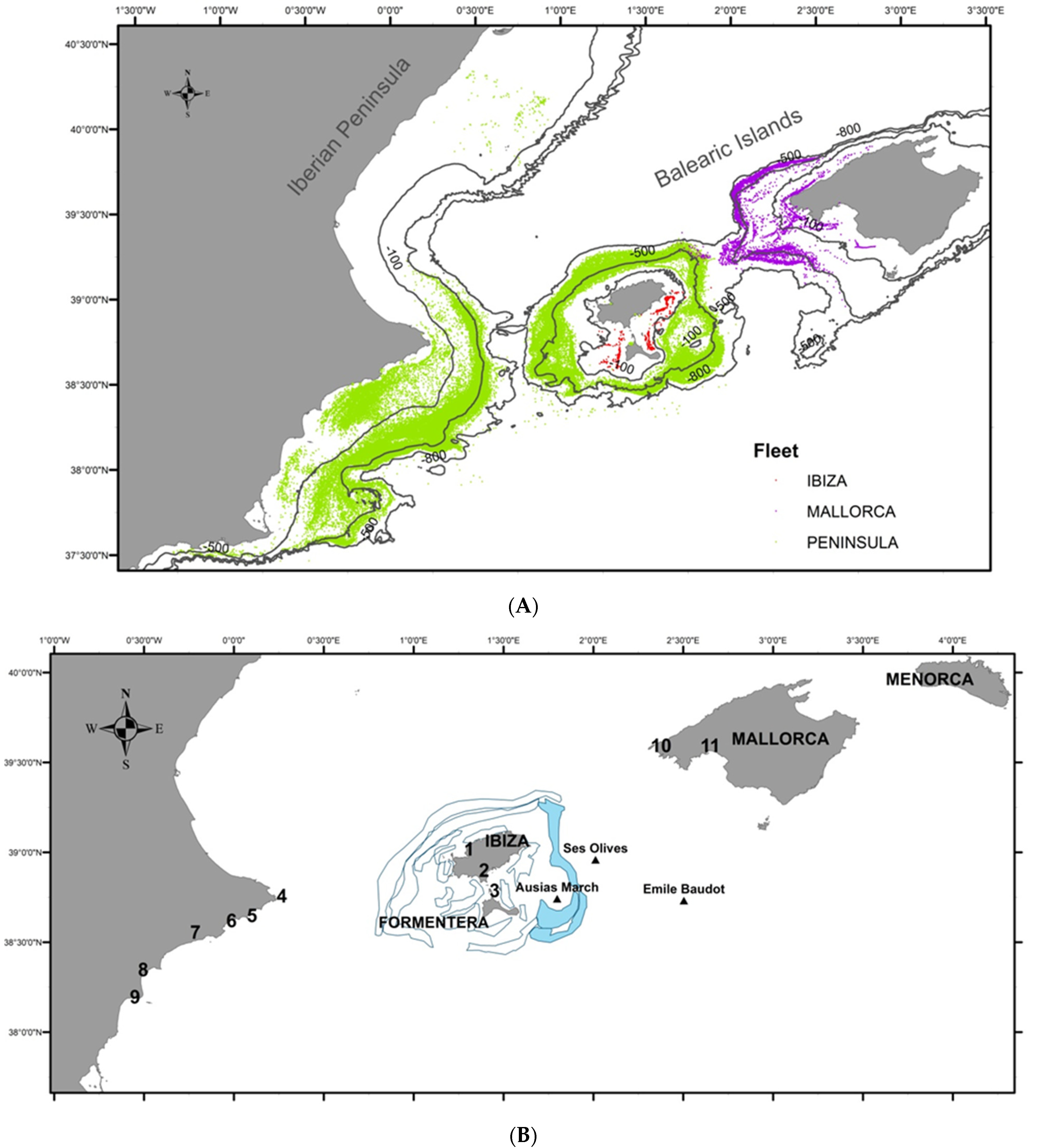
2. Study Area
3. Materials and Methods
3.1. Research Surveys
3.1.1. Geophysical Methods
3.1.2. Sediments and Rocks
3.1.3. Epi-benthos
3.1.4. Nekto-Benthos and Demersal Resources
3.1.5. Visual Transects
3.2. Fishing Activity
3.3. Analysis of Samples in the Laboratory and Data Processing
3.3.1. Geomorphology
3.3.2. Sediments
3.3.3. Biological Communities and Fishing Resources
3.3.4. Habitat Identification from Images
4. Results
4.1. Geomorphological Features of the Seafloor
- Structural features
- Fluid escape-related features
- Volcanic features
- Mass-movement related features
- Bottom current related features
- Biogenic related features
4.2. Sediment Characterization
4.3. Biodiversity, Species Assemblages and Fishing Resources
4.4. Bottom Trawling
4.5. Habitats
5. Discussion
5.1. Geodiversity
5.2. Biodiversity, Communities, and Habitats
5.3. Fisheries
5.4. Ecological Value of Mallorca Channel Seamounts
Author Contributions
Funding
Institutional Review Board Statement
Informed Consent Statement
Data Availability Statement
Acknowledgments
Conflicts of Interest
Appendix A

| Code | Dredge | Area | Latitude (N) | Longitude (E) | Depth (m) |
|---|---|---|---|---|---|
| A22B_0718_SK025 | SK | AM | 38°44.32′ | 001°46.05′ | 110 |
| A22B_0718_SK026 | SK | AM | 38°43.95′ | 001°46.58′ | 88 |
| A22B_0718_SK027 | SK | AM | 38°43.87′ | 001°46.58′ | 86 |
| A22B_0718_SK028 | SK | AM | 38°43.47′ | 001°46.85′ | 98 |
| A22B_0718_SK029 | SK | AM | 38°43.37′ | 001°46.70′ | 99 |
| A22B_0718_SK031 | SK | AM | 38°45.42′ | 001°46.34′ | 125 |
| A22B_0718_SK033 | SK | AM | 38°46.96′ | 001°45.44′ | 324 |
| A22B_0718_SK034 | SK | AM | 38°45.16′ | 001°47.01′ | 113 |
| A22B_0718_SK035 | SK | AM | 38°45.67′ | 001°49.00′ | 103 |
| A22B_0718_SK036 | SK | AM | 38°43.11′ | 001°53.45′ | 479 |
| A22B_0718_SK038 | SK | AM | 38°45.89′ | 001°47.48′ | 131 |
| A22B_0718_SK039 | SK | AM | 38°47.73′ | 001°47.66′ | 121 |
| A22B_0718_SK040 | SK | AM | 38°45.30′ | 001°48.45′ | 98 |
| A22B_0718_SK041 | SK | AM | 38°45.65′ | 001°49.60′ | 104 |
| A22B_0718_SK042 | SK | AM | 38°45.35′ | 001°49.45′ | 105 |
| A22B_0718_SK043 | SK | AM | 38°44.97′ | 001°49.51′ | 103 |
| A22B_0718_SK045 | SK | AM | 38°44.86′ | 001°51.03′ | 132 |
| A22B_0718_SK046 | SK | AM | 38°45.16′ | 001°50.89′ | 124 |
| A22B_0718_SK047 | SK | AM | 38°45.63′ | 001°51.02′ | 121 |
| A22B_0718_SK048 | SK | AM | 38°45.60′ | 001°51.68′ | 142 |
| A22B_0718_SK049 | SK | AM | 38°45.08′ | 001°52.62′ | 436 |
| A22B_1019_SK054 | SK | AM | 38°45.48′ | 001°47.71′ | 115 |
| A22B_1019_SK056 | SK | AM | 38°46.64′ | 001°52.07′ | 134 |
| A22B_1019_SK084 | SK | AM | 38°42.08′ | 001°45.77′ | 352 |
| A22B_1019_SK092 | SK | AM | 38°42.28′ | 001°44.99′ | 385 |
| A22B_1019_SK100 | SK | AM | 38°48.15′ | 001°44.75′ | 338 |
| A22B_1019_SK102 | SK | AM | 38°4815′ | 001°44.98′ | 335 |
| A22B_1019_SK106 | SK | AM | 38°4712′ | 001°51.38′ | 130 |
| A22B_0820_SK18 | SK | AM | 38°51.26′ | 001° 55.29′ | 490 |
| A22B_0820_BC20 | BC | AM | 38°48.48′ | 002°00.35′ | 667 |
| A22B_0820_SK21 | SK | AM | 38°49.98′ | 001° 53.48′ | 506 |
| A22B_0820_SK22 | SK | AM | 38°52.34′ | 001° 51.79′ | 430 |
| A22B_0820_BC23 | BC | AM | 38°50.30′ | 001°45.87′ | 341 |
| A22B_0820_SK31 | SK | AM | 38°40.22′ | 001° 47.86′ | 441 |
| A22B_0820_SK33 | SK | AM | 38°42.19′ | 001° 57.34′ | 664 |
| A22B_0718_SK053 | SK | EB | 38°44.21′ | 002°30.09 | 109 |
| A22B_0718_SK054 | SK | EB | 38°44.21′ | 002°30.15 | 107 |
| A22B_0718_SK055 | SK | EB | 38°44.23′ | 002°30.27 | 104 |
| A22B_0718_SK056 | SK | EB | 38°44.37′ | 002°30.18 | 108 |
| A22B_0718_SK057 | SK | EB | 38°44.43′ | 002°30.24 | 107 |
| A22B_0718_SK059 | SK | EB | 38°44.11′ | 002°29.52 | 128 |
| A22B_0718_SK064 | SK | EB | 38°44.94′ | 002°30.82 | 134 |
| A22B_0718_SK065 | SK | EB | 38°43.17′ | 002°29.42 | 147 |
| A22B_0718_SK070 | SK | EB | 38°41.83′ | 002°28.00 | 149 |
| A22B_0718_SK071 | SK | EB | 38°41.17′ | 002°28.11 | 153 |
| A22B_0718_SK072 | SK | EB | 38°42.05′ | 002°29.79 | 278 |
| A22B_0718_SK073 | SK | EB | 38°42.44′ | 002°29.96 | 152 |
| A22B_0718_SK074 | SK | EB | 38°42.45′ | 002°29.53 | 152 |
| A22B_0718_BC080 | BC | EB | 38°46.86′ | 002°31.12′ | 320 |
| A22B_0718_BC082 | BC | EB | 38°43.60′ | 002°28.25′ | 399 |
| A22B_0718_SK084 | SK | EB | 38°43.17′ | 002°29.45′ | 147 |
| A22B_0718_SK087 | SK | EB | 38°41.24′ | 002°26.61′ | 319 |
| A22B_0718_SK089 | SK | EB | 38°45.09′ | 002°27.65′ | 583 |
| A22B_1019_SK151 | SK | EB | 38°40.38′ | 002°26.57′ | 394 |
| A22B_1019_SK152 | SK | EB | 38°40.56′ | 002°29.02′ | 486 |
| A22B_1019_SK161 | SK | EB | 38°42.63′ | 002°27.61′ | 320 |
| A22B_1019_SK162 | SK | EB | 38°41.94′ | 002°25.11′ | 575 |
| A22B_1019_SK171 | SK | EB | 38°42.29′ | 002°28.28′ | 153 |
| A22B_1019_SK172 | SK | EB | 38°42.04′ | 002°32.43′ | 727 |
| A22B_1019_SK181 | SK | EB | 38°43.05′ | 002°30.43′ | 147 |
| A22B_1019_SK183 | SK | EB | 38°43.38′ | 002°28.28′ | 423 |
| A22B_1019_SK184 | SK | EB | 38°43.95′ | 002°31.90′ | 316 |
| A22B_1019_SK185 | SK | EB | 38°44.05′ | 002°31.17′ | 125 |
| A22B_0820_SK44 | SK | EB | 38°45.76′ | 002° 31.25′ | 326 |
| A22B_0820_SK46 | SK | EB | 38°42.15′ | 002° 26.74′ | 307 |
| A22B_0820_SK47 | SK | EB | 38°41.24′ | 002° 26.03′ | 308 |
| A22B_0820_SK48 | SK | EB | 38°41.14′ | 002° 25.98′ | 349 |
| A22B_0820_BC49 | BC | EB | 38°40.91′ | 002° 25.27′ | 285 |
| A22B_1019_SK174 | SK | CB | 38°51.89′ | 002°19.68′ | 1060 |
| A22B_1019_SK191 | SK | CB | 38°53.13′ | 002°22.51′ | 986 |
| A22B_0820_SK02 | SK | CB | 38°05.48′ | 002°09.48′ | 946 |
| A22B_0820_SK15 | SK | CB | 38°57.55′ | 002°05.48′ | 950 |
| A22B_0820_SK37 | SK | CB | 38°52.80′ | 002° 05.91′ | 852 |
| A22B_0820_SK38 | SK | CB | 38°52.62′ | 002° 08.09′ | 924 |
| A22B_0820_SK39 | SK | CB | 38°50.90′ | 002°13.69′ | 1044 |
| A22B_0718_SK002 | SK | SO | 38°57.84′ | 002°00.11′ | 286 |
| A22B_0718_SK003 | SK | SO | 38°57.57′ | 001°58.45′ | 291 |
| A22B_0718_SK004 | SK | SO | 38°59.35′ | 001°59.44′ | 627 |
| A22B_0718_SK006 | SK | SO | 38°56.28′ | 001°57.99′ | 281 |
| A22B_0718_SK007 | SK | SO | 38°55.78′ | 001°57.73′ | 265 |
| A22B_0718_SK008 | SK | SO | 38°54.56′ | 001°57.19′ | 683 |
| A22B_0718_SK009 | SK | SO | 38°54.31′ | 001°59.45′ | 661 |
| A22B_0718_BC010 | BC | SO | 38°58.80′ | 001°59.06′ | 697 |
| A22B_0718_SK013 | SK | SO | 38°59.36′ | 002°01.33′ | 1062 |
| A22B_0718_SK015 | SK | SO | 38°57.43′ | 002°00.23′ | 282 |
| A22B_0718_SK016 | SK | SO | 38°57.18′ | 002°00.28′ | 302 |
| A22B_0718_SK017 | SK | SO | 38°56.52′ | 002°00.49′ | 510 |
| A22B_1019_SK005 | SK | SO | 38°57.60′ | 001°59.40′ | 292 |
| A22B_1019_SK006 | SK | SO | 38°57.15′ | 001°58.21′ | 298 |
| A22B_1019_SK016 | SK | SO | 38°55.36′ | 001°57.38′ | 452 |
| A22B_1019_SK024 | SK | SO | 38°56.92′ | 001°59.68′ | 296 |
| A22B_1019_SK026 | SK | SO | 38°56.18′ | 001°58.93′ | 446 |
| A22B_0820_SK17 | SK | SO | 38°53.64′ | 001° 56.18′ | 688 |
| A22B_0718_SK012 | SK | PK | 38°59.86′ | 001°59.24′ | 793 |
| A22B_1019_SK030 | SK | PK | 38°54.98′ | 002°01.06′ | 786 |
| A22B_1019_SK031 | SK | PK | 38°54.99′ | 002°00.93′ | 780 |
| A22B_1019_SK038 | SK | PK | 38°57.85′ | 001°56.58′ | 617 |
| A22B_1019_SK039 | SK | PK | 38°58.14′ | 001°56.15′ | 633 |
| A22B_1019_SK110 | SK | PK | 38°55.51′ | 001°55.33′ | 667 |
| A22B_1019_SK117 | SK | PK | 38°57.33′ | 001°51.75′ | 587 |
| A22B_1019_SK118 | SK | PK | 38°57.42′ | 001°52.11′ | 638 |
| A22B_1019_BC119 | BC | PK | 38°59.80′ | 001°53.90′ | 607 |
| A22B_1019_SK121 | SK | PK | 39°00.80′ | 001°56.11′ | 710 |
| A22B_0820_SK05 | SK | PK | 39°05.44′ | 001°57.70′ | 723 |
| A22B_0820_BC08 | BC | PK | 38°58.77′ | 001°56.97′ | 656 |
| A22B_0820_BC10 | BC | PK | 38°59.20′ | 001°53.79′ | 597 |
| A22B_0820_BC12 | BC | PK | 38°53.38′ | 001°59.53′ | 749 |
| A22B_0820_SK16 | SK | PK | 38°56.34′ | 002°01.88′ | 778 |
| A22B_1019_SK042 | SK | PK | 38°32.80′ | 001°48.44′ | 628 |
| A22B_1019_SK043 | SK | PK | 38°32.96′ | 001°48.72′ | 633 |
| A22B_1019_BC068 | BC | PK | 38°33.05′ | 001°48.92′ | 630 |
| A22B_1019_SK069 | SK | PK | 38°33.19′ | 001°49.10′ | 630 |
| A22B_1019_BC070 | BC | PK | 38°32.95′ | 001°49.05′ | 629 |
| A22B_1019_BC076 | BC | PK | 38°35.74′ | 001°47.50′ | 564 |
| A22B_1019_SK077 | SK | PK | 38°36.01′ | 001°47.82′ | 556 |
| A22B_1019_BC078 | BC | PK | 38°35.68′ | 001°47.53′ | 560 |
| A22B_0820_BC26 | BC | PK | 38°40.87′ | 001°41.01′ | 390 |
| A22B_0820_SK30 | SK | PK | 38°38.47′ | 001°43.42′ | 429 |
| A22B_0820_SK32 | SK | PK | 38°36.18′ | 001°53.16′ | 624 |
| A22B_0718_BC076 | BC | PK | 38°45.58′ | 002°25.86′ | 726 |
| A22B_0718_SK078 | SK | PK | 38°47.57′ | 002°27.27′ | 721 |
| A22B_0718_BC079 | BC | PK | 38°50.07′ | 002°27.81′ | 770 |
| A22B_1019_SK131 | SK | PK | 38°48.11′ | 002°26.09′ | 739 |
| A22B_1019_SK139 | SK | PK | 38°48.97′ | 002°29.68′ | 735 |
| A22B_1019_SK140 | SK | PK | 38°49.41′ | 002°28.52′ | 431 |
| A22B_1019_SK164 | SK | PK | 38°49.52′ | 002°30.81′ | 759 |
| A22B_1019_BC190 | BC | PK | 38°53.73′ | 002°29.43′ | 755 |
| A22B_0820_SK45 | SK | PK | 38°45.77′ | 002°33.88′ | 761 |
| A22B_0820_SK51 | SK | PK | 38°40.68′ | 002°25.95′ | 316 |
| A22B_0820_SK52 | SK | PK | 38°38.56′ | 002°18.78′ | 1017 |
| A22B_0820_SK53 | SK | PK | 38°38.65′ | 002°29.22′ | 1005 |
| A22B_0820_BC54 | BC | PK | 38°39.37′ | 002°22.60′ | 905 |
| A22B_0820_SK57 | SK | PK | 38°53.03′ | 002°27.82′ | 744 |
| A22B_0820_SK58 | SK | PK | 38°49.90′ | 002°24.65′ | 798 |
| A22B_0820_SK59 | SK | PK | 38°48.57′ | 002°21.21′ | 993 |
| A22B_0820_SK60 | SK | PK | 38°47.45′ | 002°19.92′ | 985 |
| A22B_0820_SK62 | SK | PK | 38°43.83′ | 002°20.19′ | 895 |
Appendix B
| Setting | Hauling | ||||||
|---|---|---|---|---|---|---|---|
| Code | Area | Date | Latitude (N) | Longitud (E) | Latitude (N) | Longitud (E) | Depth (m) |
| A22B_0718_DR_014 | SO | 28 July 2018 | 38°58.97′ | 001°59.97′ | 38°58.74′ | 001°59.98′ | 479–278 |
| A22B_0718_DR_018 | SO | 28 July 2018 | 38°57.36′ | 002°01.09′ | 38°57.41′ | 002°00.83′ | 263–235 |
| A22B_0718_DR_019 | SO | 28 July 2018 | 38°57.01′ | 001°59.55′ | 38°57.13′ | 001°59.45′ | 278–285 |
| A22B_0718_DR_023 | AM | 30 July 2018 | 38°44.54′ | 001°46.66′ | 38°44.40′ | 001°46.85′ | 106–92 |
| A22B_0718_DR_024 | AM | 30 July 2018 | 38°43.98′ | 001°46.54′ | 38°43.99′ | 001°46.28′ | 90 |
| A22B_0718_DR_052 | EB | 3 August 2018 | 38°44.23′ | 002°30.03′ | 38°44.21′ | 002°30.20′ | 109–107 |
| A22B_0718_DR_058 | EB | 3 August 2018 | 38°43.93′ | 002°29.11′ | 38°44.00′ | 002°29.25′ | 131–126 |
| A22B_0718_DR_062 | EB | 4 August 2018 | 38°45.80′ | 002°34.33′ | 38°45.56′ | 002°34.37′ | 600–556 |
| A22B_0718_DR_067 | EB | 4 August 2018 | 38°41.54′ | 002°27.56′ | 38°41.66′ | 002°27.97′ | 144–151 |
| A22B_0718_DR_068 | EB | 4 August 2018 | 38°41.91′ | 002°28.76′ | 38°42.16′ | 002°28.59′ | 125–135 |
| A22B_0718_DR_086 | EB | 7 August 2018 | 38°40.65′ | 002°25.73′ | 38°40.65′ | 002°25.95′ | 337–309 |
| A22B_1019_DR_003 | SO | 11 October 2019 | 38°58.66′ | 001°59.29′ | 38°58.55′ | 001°59.23′ | 287–257 |
| A22B_1019_DR_008 | SO | 11 October 2019 | 38°57.65′ | 002°00.89′ | 38°57.70′ | 002°00.97′ | 253–227 |
| A22B_1019_DR_009 | SO | 11 October 2019 | 38°57.68′ | 002°00.99′ | 38°57.63′ | 002°00.92′ | 253–242 |
| A22B_1019_DR_014 | SO | 12 October 2019 | 38°55.61′ | 001°57.63′ | 38°55.69′ | 001°57.61º | 266–250 |
| A22B_1019_DR_015 | SO | 12 October 2019 | 38°55.58′ | 001°57.65′ | 38°55.68′ | 001°57.59′ | 268–241 |
| A22B_1019_DR_114 | SO | 23 October 2019 | 38°56.99′ | 001°53.23′ | 38°56.93′ | 001°53.03′ | 428–385 |
| A22B_1019_DR_051 | AM | 15 October 2019 | 38°44.15′ | 001°49.14′ | 38°44.22′ | 001°49.19′ | 105 |
| A22B_1019_DR_052 | AM | 15 October 2019 | 38°44.18′ | 001°47.64′ | 38°44.27′ | 001°47.70′ | 91–89 |
| A22B_1019_DR_053 | AM | 15 October 2019 | 38°45.05′ | 001°47.68′ | 38°44.95′ | 001°47.79′ | 107–96 |
| A22B_1019_DR_095 | AM | 19 October 2019 | 38°47.82′ | 001°52.56′ | 38°47.74′ | 001°52.38′ | 289–217 |
| A22B_1019_DR_097 | AM | 19 October 2019 | 38°48.28′ | 001°52.91′ | 38°48.35′ | 001°52.61′ | 458–352 |
| A22B_1019_DR_103 | AM | 21 October 2019 | 38°47.43′ | 001°47.17′ | 38°47.27′ | 001°47.22′ | 310–241 |
| A22B_1019_DR_128 | EB | 24 October 2019 | 38°49.32′ | 002°28.66′ | 38°49.45′ | 002°28.50′ | 607–446 |
| A22B_1019_DR_132 | EB | 25 October 2019 | 38°46.66′ | 002°27.99′ | 38°46.60′ | 002°28.07′ | 560–524 |
| A22B_1019_DR_137 | EB | 25 October 2019 | 38°44.85′ | 002°30.28′ | 38°44.83′ | 002°30.19′ | 124,114 |
| A22B_1019_DR_144 | EB | 26 October 2019 | 38°42.78′ | 002°27.72′ | 38°42.65′ | 002°27.82′ | 321–286 |
| A22B_1019_DR_147 | EB | 26 October 2019 | 38°42.23′ | 002°28.91′ | 38°42.26′ | 002°29.03′ | 126–123 |
| A22B_1019_DR_165 | EB | 28 October 2019 | 38°46.97′ | 002°31.10′ | 38°46.88′ | 002°31.13′ | 320–312 |
| A22B_1019_DR_176 | EB | 29 October 2019 | 38°45.28′ | 002°31.50′ | 38°45.23′ | 002°31.48′ | 144–141 |
| A22B_0720_DR_003 | SO | 21 July 2020 | 38°56.67′ | 001°59.94′ | 38°56.74′ | 001°59.77′ | 455–288 |
| A22B_0720_DR_004 | SO | 21 July 2020 | 38°56.39′ | 001°59.03′ | 38°56.30′ | 001°59.05′ | 440–350 |
| A22B_0720_DR_007 | SO | 21 July 2020 | 38°58.76′ | 001°59.01′ | 38°58.56 | 001°59.14′ | 384–255 |
| A22B_0720_DR_008 | SO | 21 July 2020 | 38°58.165′ | 002°00.67′ | 38°58.20′ | 002°00.43′ | 355–295 |
| A22B_0720_DR_009 | SO | 21 July 2020 | 38°58.79′ | 002°00.85′ | 38°59.04′ | 002°00.50′ | 673–657 |
| A22B_0720_DR_012 | SO | 22 July 2020 | 38°55.91′ | 001°56.09′ | 38°55.87′ | 001°56.43′ | 664–609 |
| A22B_0720_DR_014 | SO | 22 July 2020 | 38°55.51′ | 001°58.13′ | 38°55.91′ | 001°57.88′ | 395–270 |
| A22B_0720_DR_015 | SO | 22 July 2020 | 38°56.38′ | 001°59.59′ | 38°56.60′ | 001°59.35′ | 428–287 |
| A22B_0720_DR_019 | AM | 23 July 2020 | 38°43.83′ | 001°45.57′ | 38°43.77′ | 001°45.72′ | 112–94 |
| A22B_0720_DR_020 | AM | 23 July 2020 | 38°42.87′ | 001°46.47′ | 38°43.19′ | 001°46.47′ | 137–104 |
| A22B_0720_DR_027 | AM | 24 July 2020 | 38°47.55′ | 001°52.83′ | 38°47.48′ | 001°52.53′ | 226–195 |
| A22B_0720_DR_028 | AM | 24 July 2020 | 38°45.95′ | 001°51.87′ | 38°46.06′ | 001°51.76′ | 142–133 |
| A22B_0720_DR_030 | AM | 24 July 2020 | 38°47.31′ | 001°47.01′ | 38°46.97′ | 001°47.13′ | 276–204 |
| A22B_0720_DR_034 | AM | 25 July 2020 | 38°46.03′ | 001°49.09′ | 38°45.92′ | 001°49.24′ | 121–105 |
| A22B_0720_DR_042 | EB | 26 July 2020 | 38°43.54′ | 002°29.28′ | 38°43.63′ | 002°29.10′ | 139 |
| A22B_0720_DR_043 | EB | 26 July 2020 | 38°44.41′ | 002°30.66′ | 38°44.55′ | 002°30.56′ | 116 |
| A22B_0720_DR_046 | EB | 26 July 2020 | 38°42.31′ | 002°30.75′ | 38°42.52′ | 002°30.71′ | 367–235 |
| A22B_0720_DR_047 | EB | 26 July 2020 | 38°43.84′ | 002°29.40′ | 38°43.94′ | 002°29.28′ | 127 |
| A22B_0720_DR_053 | EB | 27 July 2020 | 38°44.01′ | 002°30.72′ | 38°44.14′ | 002°30.41′ | 107–102 |
| A22B_0720_DR_054 | EB | 27 July 2020 | 38°43.33′ | 002°30.90′ | 38°43.52′ | 002°30.73′ | 216–124 |
| A22B_0720_DR_057 | EB | 27 July 2020 | 38°41.72′ | 002°21.88′ | 38°41.56′ | 002°22.10′ | 665–488 |
| A22B_0720_DR_058 | EB | 27 July 2020 | 38°41.66′ | 002°29.36′ | 38°41.70′ | 002°29.27′ | 195–138 |
| A22B_0720_DR_059 | EB | 28 July 2020 | 38°42.62′ | 002°36.41′ | 38°42.85′ | 002°36.48′ | 620–550 |
| A22B_0720_DR_060 | EB | 28 July 2020 | 38°42.59′ | 002°36.63′ | 38°42.71′ | 002°36.29′ | 686–597 |
| A22B_0720_DR_061 | EB | 28 July 2020 | 38°40.70′ | 002°35.37′ | 38°40.94′ | 002°35.27′ | 1191–1066 |
Appendix C
| Setting | Hauling | Sampling | ||||||||
|---|---|---|---|---|---|---|---|---|---|---|
| Code | Area | Date | Hour | Latitude (N) | Longitud (E) | Hour | Latitude (N) | Longitud (E) | Surface (m2) | Depth (m) |
| A22B_1019_BT_002 | SO | 11 October 2019 | 7:34 | 38°57.85′ | 001°58.78′ | 7:52 | 38°57.49′ | 001°58.49′ | 654 | 295 |
| A22B_1019_BT_004 | SO | 11 October 2019 | 9:25 | 38°57.71′ | 001°59.81′ | 9:43 | 38°57.55′ | 001°59.19′ | 619 | 293 |
| A22B_1019_BT_007 | SO | 11 October 2019 | 11:23 | 38°57.33′ | 001°59.90′ | 11:41 | 38°57.65′ | 001°59.32′ | 520 | 291 |
| A22B_1019_BT_010 | SO | 11 October 2019 | 14:25 | 38°56.79′ | 001°57.71′ | 14:43 | 38°56.67′ | 001°57.65′ | 477 | 288 |
| A22B_1019_BT_012 | SO | 12 October 2019 | 6:52 | 38°56.36′ | 001°59.14′ | 7:12 | 38°55.67′ | 001°58.64′ | 613 | 453 |
| A22B_1019_BT_013 | SO | 12 October 2019 | 7:39 | 38°55.50′ | 001°57.03′ | 8:01 | 38°54.98′ | 001°58.14′ | 758 | 504 |
| A22B_1019_BT_027 | SO | 13 October 2019 | 6:12 | 38°56.85′ | 002°00.76′ | 6:32 | 38°56.48′ | 001°59.84′ | 480 | 491 |
| A22B_1019_BT_028 | SO | 13 October 2019 | 7:38 | 38°56.75′ | 002°01.16′ | 7:55 | 38°57.29′ | 002°01.32 | 487 | 449 |
| A22B_1019_BT_029 | SO | 13 October 2019 | 8:26 | 38°56.44′ | 002°01.63′ | 8:51 | 38°55.59′ | 002°01.32′ | 272 | 764 |
| A22B_1019_BT_036 | SO | 13 October 2019 | 15:51 | 38°57.19′ | 001°56.11′ | 16:18 | 38°57.99′ | 001°56.67′ | 590 | 619 |
| A22B_1019_BT_049 | AM | 15 October 2019 | 7:07 | 38°43.33′ | 001°49.37′ | 7:19 | 38°43.80′ | 001°50.09′ | 697 | 124 |
| A22B_1019_BT_050 | AM | 15 October 2019 | 7:49 | 38°43.42′ | 001°47.90′ | 8:00 | 38°43.58′ | 001°48.39′ | 524 | 102 |
| A22B_1019_BT_055 | AM | 15 October 2019 | 10:44 | 38°45.44′ | 001°47.56′ | 10:48 | 38°45.56′ | 001°47.78′ | 425 | 114 |
| A22B_1019_BT_058 | AM | 15 October 2019 | 12:40 | 38°46.54′ | 001°52.09′ | 12:53 | 38°47.10′ | 001°52.33′ | 642 | 139 |
| A22B_1019_BT_065 | AM | 16 October 2019 | 6:19 | 38°35.57′ | 001°53.45′ | 6:47 | 38°36.83′ | 001°54.40′ | 1679 | 631 |
| A22B_1019_BT_075 | AM | 17 October 2019 | 8:46 | 38°34.72′ | 001°45.22′ | 9:17 | 38°35.52′ | 001°46.80′ | 2057 | 551 |
| A22B_1019_BT_079 | AM | 17 October 2019 | 13:37 | 38°39.07′ | 001°50.42′ | 14:11 | 38°40.02′ | 001°51.82′ | 1850 | 501 |
| A22B_1019_BT_089 | AM | 18 October 2019 | 14:10 | 38°40.71′ | 001°41.94′ | 14:44 | 38°41.45′ | 001°43.28′ | 2040 | 410 |
| A22B_1019_BT_093 | AM | 19 October 2019 | 6:03 | 38°48.40′ | 001°48.03′ | 6:32 | 38°48.89′ | 001°50.45′ | 1531 | 376 |
| A22B_1019_BT_094 | AM | 19 October 2019 | 6:54 | 38°48.85′ | 001°51.06′ | 7:21 | 38° 50.02′ | 001° 51.21′ | 2123 | 409 |
| A22B_1019_BT_099 | AM | 19 October 2019 | 12:25 | 38°46.20′ | 001°48.91′ | 12:42 | 38°46.50′ | 001°49.60′ | 1241 | 131 |
| A22B_1019_BT_101 | AM | 21 October 2019 | 7:34 | 38°48.70′ | 001°42.88′ | 7:58 | 38°47.83′ | 001°42.40′ | 1056 | 320 |
| A22B_1019_BT_104 | AM | 21 October 2019 | 11:12 | 38°45.62′ | 001°50.77′ | 11:25 | 38° 46.09′ | 001°51.14′ | 524 | 116 |
| A22B_1019_BT_109 | SO | 23 October 2019 | 6:39 | 38°53.67′ | 001°55.37′ | 7:15 | 38°55.12′ | 001°56.12′ | 2086 | 715 |
| A22B_1019_BT_113 | SO | 23 October 2019 | 10:25 | 38°54.41′ | 001°56.72′ | 11:05 | 38°53.66′ | 001°58.61′ | 1991 | 697 |
| A22B_1019_BT_122 | SO | 24 October 2019 | 7:42 | 39°00.54′ | 001°55.57′ | 8:18 | 38°59.61′ | 001°57.40′ | 2148 | 693 |
| A22B_1019_BT_123 | SO | 24 October 2019 | 8:54 | 38°58.27′ | 001°55.85′ | 9:30 | 38°59.97′ | 001°56.56′ | 2222 | 675 |
| A22B_1019_BT_124 | EB | 24 October 2019 | 13:37 | 38°45.11′ | 002°31.16′ | 13:45 | 38°45.35′ | 002°31.14′ | 387 | 146 |
| A22B_1019_BT_125 | EB | 24 October 2019 | 14:18 | 38°45.61′ | 002°31.66′ | 14:36 | 38°46.06′ | 002°30.98′ | 630 | 314 |
| A22B_1019_BT_135 | EB | 25 October 2019 | 14:05 | 38°44.91′ | 002°29.66′ | 14:16 | 38°44.53′ | 002°29.27′ | 815 | 153 |
| A22B_1019_BT_136 | EB | 25 October 2019 | 14:49 | 38°42.85′ | 002°29.51′ | 15:00 | 38°43.23′ | 002°29.37′ | 689 | 143 |
| A22B_1019_BT_143 | EB | 26 October 2019 | 10:19 | 38°47.46′ | 002°30.78′ | 10:51 | 38°47.82′ | 002°29.47′ | 1271 | 686 |
| A22B_1019_BT_148 | EB | 26 October 2019 | 15:10 | 38°41.45′ | 002°28.18′ | 15:20 | 38°41.15′ | 002°28.03′ | 641 | 147 |
| A22B_1019_BT_149 | EB | 26 October 2019 | 15:49 | 38°40.76′ | 002°27.48′ | 16:08 | 38°40.96′ | 002°26.83′ | 614 | 277 |
| A22B_1019_BT_156 | EB | 27 October 2019 | 11:23 | 38°48.48′ | 002°25.14′ | 12:03 | 38°49.89′ | 002°25.70′ | 1360 | 759 |
| A22B_1019_BT_157 | EB | 27 October 2019 | 14:00 | 38°41.41′ | 002°26.95′ | 14:20 | 38°42.20′ | 002°27.09′ | 1135 | 288 |
| A22B_1019_BT_158 | EB | 27 October 2019 | 14:57 | 38°42.97′ | 002°29.65′ | 15:07 | 38°42.94′ | 002°29.11′ | 524 | 143 |
| A22B_1019_BT_166 | EB | 28 October 2019 | 14:47 | 38°44.48′ | 002°28.48′ | 15:08 | 38°43.74′ | 002°28.03′ | 1295 | 433 |
| A22B_1019_BT_167 | EB | 28 October 2019 | 15:44 | 38°42.54′ | 002°29.77′ | 15:55 | 38°42.22′ | 002°29.50′ | 655 | 151 |
| A22B_1019_BT_175 | EB | 29 October 2019 | 11:47 | 38°46.07′ | 002°30.15′ | 12:08 | 38°46.53′ | 002°31.10′ | 1182 | 412 |
| A22B_1019_BT_177 | EB | 29 October 2019 | 14:22 | 38°44.23′ | 002°28.89′ | 14:34 | 38°43.79′ | 002°28.90′ | 644 | 156 |
| A22B_1019_BT_178 | EB | 29 October 2019 | 15:09 | 38°43.21′ | 002°27.37′ | 15:35 | 38°43.32′ | 002°26.27′ | 1262 | 555 |
| A22B_1019_BT_188 | EB | 30 October 2019 | 13:18 | 38°49.11′ | 002°28.94′ | 13:44 | 38°50.01′ | 002°30.21′ | 2497 | 753 |
| A22B_0718_BT_001 | SO | 27 July 2018 | 6:40 | 38°56.80′ | 001°58.54′ | 7:03 | 38°57.38′ | 001°59.39′ | 849 | 290 |
| A22B_0718_BT_005 | SO | 27 July 2018 | 13:58 | 38°58.62′ | 001°59.88′ | 14:18 | 38°58.12′ | 001°59.24′ | 760 | 259 |
| A22B_0718_BT_020 | SO | 28 July 2018 | 16:52 | 38°56.10′ | 001°58.52′ | 17:11 | 38°56.10′ | 001°57.73′ | 691 | 275 |
| A22B_0718_BT_021 | SO | 28 July 2018 | 18:48 | 38°56.59′ | 001°57.03′ | 19:08 | 38°57.26′ | 001°57.31′ | 603 | 489 |
| A22B_0718_BT_022 | AM | 30 July 2018 | 10:03 | 38°44.57′ | 001°46.25′ | 10:12 | 38°44.42′ | 001°45.89′ | 692 | 105 |
| A22B_0718_BT_030 | AM | 30 July 2018 | 14:12 | 38°45.47′ | 001°45.58′ | 14:26 | 38°45.84′ | 001°46.01′ | 621 | 242 |
| A22B_0718_BT_032 | AM | 30 July 2018 | 13:32 | 38°46.70′ | 001°44.90′ | 13:49 | 38°47.09′ | 001°45.45′ | 684 | 319 |
| A22B_0718_BT_037 | AM | 31 July 2018 | 8:05 | 38°45.85′ | 001°47.26′ | 8:15 | 38°45.96′ | 001°47.58′ | 694 | 124 |
| A22B_0718_BT_044 | AM | 31 July 2018 | 11:02 | 38°44.46′ | 001°50.85′ | 11:13 | 38°44.85′ | 001°50.95′ | 728 | 122 |
| A22B_0718_BT_050 | AM | 31 July 2018 | 14:22 | 38°42.27′ | 001°52.18′ | 14:45 | 38°42.95′ | 001°52.57′ | 729 | 445 |
| A22B_0718_BT_051 | EB | 3 August 2018 | 10:30 | 38°44.84′ | 002°30.52′ | 10:41 | 38°44.98′ | 002°30.91′ | 713 | 127 |
| A22B_0718_BT_060 | EB | 3 August 2018 | 17:18 | 38°43.38′ | 002°29.64′ | 17:29 | 38°43.09′ | 002°29.34′ | 637 | 137 |
| A22B_0718_BT_063 | EB | 4 August 2018 | 10:54 | 38°45.96′ | 002°34.56′ | 11:25 | 38°46.50′ | 002°35.72′ | 729 | 759 |
| A22B_0718_BT_066 | EB | 4 August 2018 | 14:06 | 38°41.42′ | 002°28.44′ | 14:19 | 38°41.12′ | 002°28.03′ | 618 | 146 |
| A22B_0718_BT_069 | EB | 4 August 2018 | 16:00 | 38°41.98′ | 002°28.21′ | 16:12 | 38°41.73′ | 002°27.86′ | 755 | 146 |
| A22B_0718_BT_077 | EB | 6 August 2018 | 9:24 | 38°46.24′ | 002°26.01′ | 9:50 | 38°46.95′ | 002°26.65′ | 740 | 704 |
| A22B_0718_BT_085 | EB | 7 August 2018 | 8:12 | 38°41.92′ | 002°26.71′ | 8:31 | 38°41.29′ | 002°26.62′ | 624 | 299 |
| A22B_0718_BT_088 | EB | 7 August 2018 | 11:00 | 38°45.48′ | 002°27.75′ | 11:23 | 38°44.74′ | 002°27.44′ | 698 | 574 |
| A22B_0720_BT_001 | SO | 21 July 2020 | 6:12 | 38°57.67′ | 002°00.64′ | 6:33 | 38°58.25′ | 002°00.00′ | 1443 | 281 |
| A22B_0720_BT_002 | SO | 21 July 2020 | 7:09 | 38°57.29′ | 002°00.40′ | 7:31 | 38°56.96′ | 001°59.60′ | 1229 | 298 |
| A22B_0720_BT_005 | SO | 21 July 2020 | 11:31 | 38°56.57′ | 001°57.25′ | 11:56 | 38°55.90′ | 001°56.60′ | 1172 | 405 |
| A22B_0720_BT_006 | SO | 21 July 2020 | 12:39 | 38°57.46′ | 001°57.06′ | 13:16 | 38°58.28′ | 001°58.16′ | 1901 | 556 |
| A22B_0720_BT_010 | SO | 22 July 2020 | 6:06 | 38°54.47′ | 001°56.28′ | 6:45 | 38°55.45′ | 001°56.80′ | 1900 | 697 |
| A22B_0720_BT_011 | SO | 22 July 2020 | 7:49 | 38°55.64′ | 001°55.99′ | 8:26 | 38°54.37′ | 001°55.46′ | 1848 | 715 |
| A22B_0720_BT_013 | SO | 22 July 2020 | 11:27 | 38°56.48′ | 001°56.00′ | 12:01 | 38°57.71′ | 001°56.30′ | 1768 | 607 |
| A22B_0720_BT_016 | AM | 23 July 2020 | 7:00 | 38°43.40′ | 001°47.04′ | 7:14 | 38°43.25′ | 001°46.64′ | 949 | 99 |
| A22B_0720_BT_017 | AM | 23 July 2020 | 7:52 | 38°45.39′ | 001°47.08′ | 8:11 | 38°45.08′ | 001°46.60′ | 1067 | 112 |
| A22B_0720_BT_018 | AM | 23 July 2020 | 8:41 | 38°45.05′ | 001°46.55′ | 8:57 | 38°45.27′ | 001°46.90′ | 165 | 113 |
| A22B_0720_BT_021 | AM | 23 July 2020 | 14:17 | 38°44.92′ | 001°50.16′ | 14:34 | 38°45.32′ | 001°50.49′ | 477 | 105 |
| A22B_0720_BT_026 | AM | 24 July 2020 | 9:11 | 38°47.16′ | 001°50.76′ | 9:27 | 38°47.10′ | 001°51.44′ | 281 | 127 |
| A22B_0720_BT_029 | AM | 24 July 2020 | 12:43 | 38°46.24′ | 001°47.57′ | 13:07 | 38°46.03′ | 001°46.52′ | 1068 | 195 |
| A22B_0720_BT_031 | AM | 24 July 2020 | 14:26 | 38°48.05′ | 001°48.19′ | 15:24 | 38°47.72′ | 001°47.08′ | 1138 | 348 |
| A22B_0720_BT_033 | AM | 25 July 2020 | 6:57 | 38°46.73′ | 001°47.67′ | 7:19 | 38°47.37′ | 001°48.27′ | 1173 | 225 |
| A22B_0720_BT_035 | AM | 25 July 2020 | 8:52 | 38°44.42′ | 001°43.79′ | 9:23 | 38°43.80′ | 001°42.75′ | 849 | 352 |
| A22B_0720_BT_037 | AM | 25 July 2020 | 11:15 | 38°42.86′ | 001°51.53′ | 11:49 | 38°42.05′ | 001°50.73′ | 1200 | 363 |
| A22B_0720_BT_038 | EB | 26 July 2020 | 6:09 | 38°43.72′ | 002°27.69′ | 6:38 | 38°42.52′ | 002°27.67′ | 846 | 511 |
| A22B_0720_BT_039 | EB | 26 July 2020 | 7:49 | 38°44.84′ | 002°28.28′ | 8:13 | 38°44.21′ | 002°27.84′ | 936 | 483 |
| A22B_0720_BT_044 | EB | 26 July 2020 | 11:57 | 38°39.11′ | 002°29.45′ | 12:34 | 38°38.97′ | 002°27.70′ | 1142 | 680 |
| A22B_0720_BT_045 | EB | 26 July 2020 | 13:40 | 38°42.52′ | 002°29.74′ | 14:01 | 38°42.27′ | 002°29.40′ | 178 | 150 |
| A22B_0720_BT_052 | EB | 27 July 2020 | 8:30 | 38°45.54′ | 002°31.59′ | 8:53 | 38°45.95′ | 002°30.62′ | 1267 | 297 |
| A22B_0720_BT_055 | EB | 27 July 2020 | 11:42 | 38°39.98′ | 002°28.99′ | 12:08 | 38°40.24′ | 002°27.81′ | 673 | 473 |
| A22B_0720_BT_062 | EB | 28 July 2020 | 12:20 | 38°43.25′ | 002°27.82′ | 12:47 | 38°44.00′ | 002°27.68′ | 894 | 508 |
Appendix D
| Setting | Hauling | Sampling | ||||||||
|---|---|---|---|---|---|---|---|---|---|---|
| Code | Area | Date | Hour | Latitude (N) | Longitude (E) | Hour | Latitude (N) | Longitude (E) | Surface (km2) | Depth (m) |
| A22B_1019_GOC_040 | AM | 14 October 2019 | 6:46 | 38°36.89′ | 001°55.19′ | 8:30 | 38°33.31′ | 001°50.91′ | 0.103084 | 631 |
| A22B_1019_GOC_044 | AM | 14 October 2019 | 11:40 | 38°30.34′ | 001°45.14′ | 13:25 | 38°33.05′ | 001°51.71′ | 0.102621 | 663 |
| A22B_1019_GOC_066 | AM | 16 October 2019 | 7:36 | 38°40.94′ | 001°56.27′ | 9:10 | 38°36.23′ | 001°53.57′ | 0.106566 | 619 |
| A22B_1019_GOC_067 | AM | 16 October 2019 | 10:50 | 38°40.64′ | 001°55.64′ | 12:30 | 38°36.17′ | 001°52.66′ | 0.097698 | 600 |
| A22B_1019_GOC_074 | AM | 17 October 2019 | 6:06 | 38°36.64′ | 001°53.26′ | 7:40 | 38°34.07′ | 001°48.65′ | 0.097105 | 601 |
| A22B_1019_GOC_085 | AM | 18 October 2019 | 6:00 | 38°35.67′ | 001°42.97′ | 7:25 | 38°38.09′ | 001°47.64′ | 0.101040 | 510 |
| A22B_1019_GOC_088 | AM | 18 October 2019 | 11:14 | 38°38.48′ | 001°39.06′ | 12:45 | 38°39.94′ | 001°44.78′ | 0.095595 | 444 |
| A22B_1019_GOC_108 | AM | 21 October 2019 | 14:55 | 38°48.53′ | 001°42.51′ | 16:24 | 38°44.14′ | 001°40.75′ | 0.099932 | 328 |
| A22B_1019_GOC_129 | EB | 25 October 2019 | 6:02 | 38°53.72′ | 002°29.05′ | 7:26 | 38°49.30′ | 002°27.71′ | 0.076988 | 756 |
| A22B_1019_GOC_130 | EB | 25 October 2019 | 8:25 | 38°51.68′ | 002°29.61′ | 9:30 | 38°48.96′ | 002°26.96′ | 0.052205 | 750 |
| A22B_1019_GOC_141 | EB | 26 October 2019 | 5:55 | 38°47.05′ | 002°27.07′ | 7:15 | 38°49.74′ | 002°31.32′ | 0.074393 | 738 |
| A22B_1019_GOC_142 | EB | 26 October 2019 | 7:58 | 38°50.73′ | 002°32.30′ | 9:15 | 38°48.13′ | 02º28.75′ | 0.073824 | 729 |
| A22B_1019_GOC_153 | EB | 28 October 2019 | 6:49 | 38°47.70′ | 002°24.46′ | 8:15 | 38°47.75′ | 002°35.20′ | 0.076893 | 768 |
| A22B_1019_GOC_154 | EB | 27 October 2019 | 9:10 | 38°52.46′ | 002°27.08′ | 10:30 | 38°51.79′ | 002°26.11′ | 0.071558 | 760 |
| A22B_1019_GOC_155 | EB | 27 October 2019 | 6:47 | 38°51.92′ | 002°33.42′ | 8:10 | 38°48.95′ | 002°25.94′ | 0.071789 | 755 |
| A22B_1019_GOC_173 | EB | 29 October 2019 | 6:53 | 38°47.34′ | 002°13.04′ | 8:40 | 38°51.19′ | 002°16.90′ | 0.093264 | 1028 |
| A22B_1019_GOC_186 | EB | 30 October 2019 | 9:20 | 38°53.16′ | 002°34.81′ | 11:00 | 38°49.24′ | 002°30.41′ | 0.103130 | 759 |
| MEDITS_0620_GOC_108 | EB | 24 June 2020 | 5:53 | 38°52.52′ | 002°27.06′ | 7:11 | 38°48.31′ | 002°25.72′ | 0.075247 | 746 |
| MEDITS_0620_GOC_109 | EB | 24 June 2020 | 7:54 | 38°47.45′ | 002°24.32′ | 9:16 | 38°51.73′ | 002°26.08′ | 0.073746 | 754 |
| MEDITS_0620_GOC_110 | EB | 24 June 2020 | 10:52 | 38°46.89′ | 002°26.75′ | 12:14 | 38°49.73′ | 002°31.30′ | 0.079473 | 732 |
| MEDITS_0621_GOC_235 | EB | 23 June 2021 | 5:56 | 38°53.15′ | 002°34.78′ | 7:19 | 38°49.64′ | 002°30.99′ | 0.088226 | 757 |
| MEDITS_0621_GOC_236 | EB | 23 June 2021 | 8:08 | 38°52.58′ | 002°30.34′ | 9:30 | 38°48.92′ | 002°26.92′ | 0.088505 | 747 |
| MEDITS_0821_GOC_003 | AM | 18 August 2021 | 11:25 | 38°34.27′ | 001°39.32′ | 12:48 | 38°34.47′ | 001°44.80′ | 0.095555 | 542 |
| MEDITS_0821_GOC_004 | AM | 18 August 2021 | 13:44 | 38°31.08′ | 001°43.56′ | 15:03 | 38°32.72′ | 001°48.91′ | 0.950162 | 627 |
| MEDITS_0821_GOC_009 | AM | 19 August 2021 | 13:01 | 38°56.65′ | 001°49.37′ | 14:30 | 38°53.04′ | 001°53.47′ | 0.113673 | 459 |
| MEDITS_0821_GOC_032 | AM | 25 August 2021 | 5:59 | 38°39.40′ | 001°55.89′ | 7:19 | 38°43.95′ | 001°56.83′ | 0.087158 | 615 |
| MEDITS_0821_GOC_033 | AM | 25 August 2021 | 8:05 | 38°45.83′ | 001°53.62′ | 9:26 | 38°41.67′ | 001°52.06′ | 0.100025 | 460 |
| MEDITS_0821_GOC_034 | AM | 25 August 2022 | 10:59 | 38°39.17′ | 001°40.08′ | 12:10 | 38°42.67′ | 001°42.62′ | 0.088374 | 393 |
| MEDITS_0821_GOC_035 | AM | 25 August 2021 | 12:55 | 38°45.88′ | 001°46.13′ | 13:45 | 38°46.91′ | 001°49.38′ | 0.053231 | 237 |
Appendix E
| Initial | Final | ||||||||||
|---|---|---|---|---|---|---|---|---|---|---|---|
| Code | Area | Date | Hour | Latitude (N) | Longitude (E) | Depth (m) | Hour | Latitude (N) | Longitude (E) | Depth (m) | Sampling Area (m2) |
| TR017 | SO | 12 October 2019 | 11:21 | 38°57.994′ | 01°58.627′ | 283 | 11:36 | 38°57.936′ | 01°58.622′ | 288 | 534.00 |
| TR018 | SO | 12 October 2019 | 11:51 | 38°57.788′ | 01°59.094′ | 288 | 12:08 | 38°57.726′ | 01°59.238′ | 287 | 602.16 |
| TR019 | SO | 12 October 2019 | 12:27 | 38°57.587′ | 01°59.551′ | 287 | 12:42 | 38°57.514′ | 01°59.720′ | 286 | 540.34 |
| TR020 | SO | 12 October 2019 | 13:25 | 38°58.410′ | 02°00.127′ | 280 | 13:45 | 38°58.298′ | 02°00.308′ | 302 | 711.18 |
| TR021 | SO | 12 October 2019 | 14:18 | 38°57.399′ | 02°00.888′ | 230 | 14:40 | 38°57.303′ | 02°01.091′ | 326 | 799.34 |
| TR022 | SO | 12 October 2019 | 15:17 | 38°56.960′ | 01°59.600′ | 284 | 15:37 | 38°56.862′ | 01°59.802′ | 292 | 687.32 |
| TR032 | SO | 13 October 2019 | 12:07 | 38°58.668′ | 01°58.213′ | 587 | 12:12 | 38°58.715′ | 01°58.160′ | 612 | 360.52 |
| TR033 | SO | 13 October 2019 | 12:50 | 38°58.600′ | 01°58.240′ | 579 | 12:58 | 38°58.678′ | 01°58.205′ | 693 | 326.72 |
| TR034 | SO | 13 October 2019 | 13:31 | 38°58.632′ | 01°58.243′ | 580 | 13:36 | 38°58.660′ | 01°58.205′ | 599 | 187.81 |
| TR035 | SO | 13 October 2019 | 14:13 | 38°58.617′ | 01°58.233′ | 583 | 14:24 | 38°58.662′ | 01°58.170′ | 621 | 335.32 |
| TR045 | AM | 14 October 2019 | 14:57 | 38°32.801′ | 01°48.446′ | 624 | 15:12 | 38°32.875′ | 01°48.568′ | 624 | 544.34 |
| TR046 | AM | 14 October 2019 | 15:35 | 38°33.073′ | 01°48.918′ | 579 | 15:50 | 38°33.140′ | 01°49.035′ | 622 | 545.80 |
| TR047 | AM | 14 October 2019 | 16:09 | 38°33.277′ | 01°49.333′ | 619 | 16:24 | 38°33.354′ | 01°49.468′ | 617 | 609.81 |
| TR059 | AM | 15 October 2019 | 14:03 | 38°44.644′ | 01°48.533′ | 94 | 14:18 | 38°44.695′ | 01°48.388′ | 92. | 629.58 |
| TR060 | AM | 15 October 2019 | 14:48 | 38°44.846′ | 01°47.938′ | 90 | 15:03 | 38°44.898′ | 01°47.791′ | 94 | 638.56 |
| TR061 | AM | 15 October 2019 | 15:21 | 38°45.040′ | 01°47.380′ | 106 | 15:36 | 38°45.092′ | 01°47.231′ | 107 | 728.32 |
| TR062 | AM | 15 October 2019 | 16:07 | 38°47.397′ | 01°44.038′ | 88 | 16:22 | 38°44.099′ | 01°47.248′ | 87 | 593.34 |
| TR063 | AM | 15 October 2019 | 16:40 | 38°44.265′ | 01°46.819′ | 90 | 16:55 | 38°44.322′ | 01°46.675′ | 90 | 634.50 |
| TR064 | AM | 15 October 2019 | 17:14 | 38°44.486′ | 01°46.263′ | 110 | 17:29 | 38°44.544′ | 01°46.121′ | 111 | 623.60 |
| TR071 | AM | 16 October 2019 | 16:41 | 38°30.436′ | 01°42.765′ | 669 | 17:01 | 38°30.340′ | 01°42.666′ | 699 | 355.56 |
| TR072 | AM | 16 October 2019 | 17:03 | 38°30.328′ | 01°42.655′ | 699 | 17:23 | 38°30.195′ | 01°42.537′ | 716 | 678.44 |
| TR073 | AM | 16 October 2019 | 17:24 | 38°30.188′ | 01°42.532′ | 717 | 17:34 | 38°30.121′ | 01°42.471′ | 727 | 342.86 |
| TR080 | AM | 17 October 2019 | 15:21 | 38°42.782′ | 01°47.863′ | 151 | 15:41 | 38°42.619′ | 01°47.867′ | 225 | 633.50 |
| TR081 | AM | 17 October 2019 | 15:43 | 38°42.607′ | 01°47.867′ | 229 | 16:03 | 38°42.441′ | 01°47.872′ | 265 | 638.76 |
| TR082 | AM | 17 October 2019 | 16:05 | 38°42.435′ | 01°47.872′ | 269 | 16:25 | 38°42.259′ | 01°47.876′ | 293 | 638.72 |
| TR086 | AM | 18 October 2019 | 9:04 | 38°43.671′ | 01°45.650′ | 95 | 9:24 | 38°43.676′ | 01°45.436′ | 657 | 656.98 |
| TR087 | AM | 18 October 2019 | 9:26 | 38°43.676′ | 01°45.429′ | 159 | 9:46 | 38°43.681′ | 01°45.200′ | 657 | 657.48 |
| TR090 | AM | 18 October 2019 | 15:40 | 38°42.058′ | 01°45.867′ | 346 | 15:55 | 38°42.095′ | 01°45.716′ | 500 | 499.58 |
| TR091 | AM | 18 October 2019 | 16:19 | 38°42.293′ | 01°45.146′ | 367 | 16:34 | 38°42.248′ | 01°45.146′ | 482 | 481.60 |
| TR096 | AM | 19 October 2019 | 9:23 | 38°48.338′ | 01°52.670′ | 339 | 9:43 | 38°48.285′ | 01°52.880′ | 691 | 691.42 |
| TR098 | AM | 19 October 2019 | 11:27 | 38°47.691′ | 01°52.250′ | 198 | 11:47 | 38°47.777′ | 01°52.443′ | 668 | 667.84 |
| TR107 | AM | 21 October 2019 | 13:58 | 38°47.246′ | 01°47.193′ | 234 | 14:18 | 38°47.403′ | 01°47.147′ | 303 | 671.60 |
| TR111 | SO | 23 October 2019 | 8:59 | 38°54.672′ | 01°56.847′ | 664 | 9:19 | 38°54.562′ | 01°56.722′ | 665 | 1113.30 |
| TR112 | SO | 23 October 2019 | 9:47 | 38°54.206′ | 01°56.389′ | 681 | 9:52 | 38°54.244′ | 01°56.375′ | 680 | 271.34 |
| TR115 | SO | 23 October 2019 | 14:16 | 38°56.829′ | 01°53.156′ | 394 | 14:36 | 38°56.827′ | 01°52.944′ | 484 | 889.36 |
| TR116 | SO | 23 October 2019 | 14:38 | 38°56.827′ | 01°52.922′ | 492 | 14:58 | 38°56.829′ | 01°52.714′ | 576 | 946.00 |
| TR126 | EB | 24 October 2019 | 15:34 | 38°49.437′ | 02°28.508′ | 426 | 15:54 | 38°56.827′ | 01°52.944′ | 580 | 880.22 |
| TR127 | EB | 24 October 2019 | 15:55 | 38°49.352′ | 02°28.323′ | 593 | 16:15 | 38°49.269′ | 02°28.175′ | 713 | 943.64 |
| TR133 | EB | 25 October 2019 | 12:59 | 38°43.847′ | 02°29.414′ | 128 | 13:19 | 38°43.970′ | 02°29.267′ | 125 | 731.20 |
| TR134 | EB | 25 October 2019 | 13:22 | 38°43.256′ | 02°29.094′ | 125 | 13:42 | 38°44.095′ | 02°29.094′ | 134 | 724.98 |
| TR145 | EB | 26 October 2019 | 13:38 | 38°42.146′ | 02°29.219′ | 131 | 13:53 | 38°42.208′ | 02°29.082′ | 123 | 525.56 |
| TR146 | EB | 26 October 2019 | 14:02 | 38°42.245′ | 02°29.000′ | 123 | 14:17 | 38°42.307′ | 02°28.862′ | 130 | 516.90 |
| TR159 | EB | 27 October 2019 | 15:52 | 38°43.770′ | 02°29.525′ | 126 | 16:12 | 38°43.762′ | 02°29.313′ | 128 | 661.86 |
| TR160 | EB | 27 October 2019 | 16:20 | 38°43.758′ | 02°29.227′ | 128 | 16:40 | 38°43.751′ | 02°29.017′ | 148 | 656.76 |
| TR168 | EB | 28 October 2019 | 16:28 | 38°42.043′ | 02°29.260′ | 138 | 16:48 | 38°42.037′ | 02°29.048′ | 131 | 656.56 |
| TR169 | EB | 28 October 2019 | 16:58 | 38°42.034′ | 02°28.945′ | 123 | 17:18 | 38°42.027′ | 02°28.738′ | 128 | 631.40 |
| TR179 | EB | 29 October 2019 | 16:32 | 38°43.368′ | 02°29.966′ | 131 | 16:52 | 38°43.375′ | 02°30.170′ | 124 | 644.68 |
| TR180 | EB | 29 October 2019 | 17:04 | 38°43.378′ | 02°30.293′ | 126 | 17:24 | 38°43.383′ | 02°30.506′ | 126 | 660.68 |
Appendix F
| Initial | Final | ||||||||||
|---|---|---|---|---|---|---|---|---|---|---|---|
| Code | Area | Date | Hour | Latitude (N) | Longitude (E) | Depth (m) | Hour | Latitude (N) | Longitude (E) | Depth (m) | Sampling Area (m2) |
| R1_1 | SO | 21 August 2020 | 12:38:25 | 38°58.98′ | 001°58.78′ | 608 | 14:47:27 | 38°58.72′ | 001°58.18′ | 637 | 784,624 |
| R1_2 | SO | 21 August 2020 | 15:33:42 | 38°58.73′ | 001°58.18′ | 642 | 16:21:43 | 38°58.99′ | 001°58.78′ | 611 | 1,086,012 |
| R1_3 | SO | 21 August 2020 | 16:31:04 | 38°58.96′ | 001°58.78′ | 800 | 16:57:00 | 38°58.92′ | 001°58.67′ | 601 | 188,041 |
| R2_1 | SO | 22 August 2020 | 8:40:40 | 38°58.95′ | 001°58.81′ | 580 | 9:48:47 | 38°58.69′ | 001°58.20′ | 611 | 1,559,742 |
| R2_2 | SO | 22 August 2020 | 10:28:07 | 38°58.76′ | 001°58.08′ | 672 | 11:34:43 | 38°58.65′ | 001°58.20′ | 604 | 229,906 |
| R3 | SO | 23 August 2020 | 7:50:31 | 38°58.65′ | 001°58.20′ | 605 | 11:42:20 | 38°58.67′ | 001°58.13′ | 640 | 241,508 |
| R4_1 | SO | 23 August 2020 | 13:58:13 | 38°56.38′ | 001°59.58′ | 423 | 15:40:40 | 38°56.47′ | 001°59.48′ | 280 | 154,396 |
| R4_2 | SO | 23 August 2020 | 16:14:04 | 38°56.59′ | 001°59.86′ | 454 | 17:10:32 | 38°56.73′ | 001°59.75′ | 289 | 299,956 |
| R5_1 | SO | 24 August 2020 | 8:09:24 | 38°56.82′ | 002°00.35′ | 443 | 9:24:59 | 38°57.00′ | 002°00.24′ | 298 | 323,297 |
| R5_2 | SO | 24 August 2020 | 10:07:51 | 38°56.96′ | 002°00.81′ | 374 | 11:28:24 | 38°57.21′ | 002°00.74′ | 254 | 385,623 |
| R6_1 | SO | 24 August 2020 | 13:38:50 | 38°57.07′ | 001°56.14′ | 606 | 14:45:44 | 38°57.47′ | 001°56.24′ | 605 | 912,376 |
| R6_2 | SO | 24 August 2020 | 15:39:11 | 38°57.53′ | 001°55.93′ | 645 | 16:53:33 | 38°57.57′ | 001°55.87′ | 624 | 101,768 |
| R7 | AM | 25 August 2020 | 7:42:33 | 38°45.74′ | 001°46.01′ | 242 | 9:48:00 | 38°45.37′ | 001°46.36′ | 120 | 799,572 |
| R8 | AM | 25 August 2020 | 10:46:55 | 38°44.44′ | 001°46.34′ | 107 | 12:53:06 | 38°44.13′ | 001°46.73′ | 86 | 719,893 |
| R9 | AM | 25 August 2020 | 13:40:29 | 38°43.92′ | 001°46.74′ | 85 | 15:10:00 | 38°44.18′ | 001°47.24′ | 85 | 925,759 |
| R10 | AM | 25 August 2020 | 16:05:07 | 38°45.38′ | 001°45.41′ | 251 | 17:17:51 | 38°45.10′ | 001°45.84′ | 128 | 687,313 |
| R11 | AM | 26 August 2020 | 7:08:53 | 38°46.96′ | 001°46.68′ | 299 | 8:51:42 | 38°46.85′ | 001°47.00′ | 197 | 528,920 |
| R12 | AM | 26 August 2020 | 10:06:05 | 38°47.30′ | 001°53.08′ | 445 | 11:39:18 | 38°47.19′ | 001°52.68′ | 215 | 504,425 |
| R13 | AM | 26 August 2020 | 12:39:20 | 38°48.37′ | 001°52.95′ | 456 | 14:11:54 | 38°48.43′ | 001°52.65′ | 344 | 435,245 |
| R14 | AM | 26 August 2020 | 15:44:22 | 38°49.99′ | 001°58.75′ | 647 | 16:39:05 | 38°50.00′ | 001°58.67′ | 630 | 113,915 |
| R15 | EB | 27 August 2020 | 6:48:54 | 38°42.29′ | 002°31.12′ | 546 | 8:17:14 | 38°42.52′ | 002°30.71′ | 233 | 708,701 |
| R16 | EB | 27 August 2020 | 9:11:44 | 38°43.10′ | 002°31.25′ | 401 | 12:01:00 | 38°43.15′ | 002°30.46′ | 143 | 1,243,278 |
| R17 | EB | 27 August 2020 | 13:04:58 | 38°44.03′ | 002°33.01′ | 593 | 14:58:32 | 38°43.89′ | 002°32.67′ | 363 | 475,220 |
| R18 | EB | 27 August 2020 | 16:03:34 | 38°44.75′ | 002°31.87′ | 500 | 17:05:37 | 38°44.76′ | 002°31.85′ | 341 | 557,222 |
| R19 | EB | 28 August 2020 | 7:01:25 | 38°40.64′ | 002°34.84′ | 1140 | 8:45:34 | 38°40.97′ | 002°34.86′ | 1015 | 524,461 |
| R20 | EB | 28 August 2020 | 10:38:16 | 38°42.74′ | 002°37.14′ | 895 | 13:20:57 | 38°42.67′ | 002°36.51′ | 523 | 765,042 |
| R21 | EB | 28 August 2020 | 15:02:34 | 38°47.61′ | 002°32.83′ | 719 | 16:57:40 | 38°47.26′ | 002°32.94′ | 417 | 661,131 |
| R22 | EB | 29 August 2020 | 8:23:53 | 38°43.90′ | 002°27.63′ | 537 | 8:22:57 | 38°43.95′ | 002°28.46′ | 287 | 996,950 |
| R23 | EB | 29 August 2020 | 9:21:25 | 38°44.45′ | 002°29.24′ | 165 | 11:27:16 | 38°44.66′ | 002°29.72′ | 129 | 738,266 |
| R24 | EB | 29 August 2020 | 12:40:32 | 38°44.76′ | 002°29.46′ | 151 | 14:25:19 | 38°44.95′ | 002°29.90′ | 130 | 682,976 |
| R25 | EB | 29 August 2020 | 15:31:19 | 38°43.91′ | 002°30.16′ | 114 | 17:06:42 | 38°44.14′ | 002°30.60′ | 96 | 652,233 |
| R26_1 | EB | 30 August 2020 | 8:19:50 | 38°52.35′ | 002°30.43′ | 740 | 9:32:20 | 38°52.89′ | 002°30.56′ | 738 | 950,914 |
| R26_2 | EB | 30 August 2020 | 10:24:19 | 38°53.08′ | 002°30.95′ | 732 | 11:50:26 | 38°53.25′ | 002°30.68′ | 515 | 374,714 |
| R27 | EB | 30 August 2020 | 13:13:58 | 38°53.73′ | 002°29.43′ | 753 | 14:42:44 | 38°53.67′ | 002°29.56′ | 700 | 150,203 |
| R28 | SO | 31 August 2020 | 7:10:43 | 38°55.84′ | 001°53.59′ | 610 | 8:35:27 | 38°55.90′ | 001°53.43′ | 587 | 176,282 |
| R29 | SO | 31 August 2020 | 9:49:08 | 85°6.974′ | 001°53.57′ | 422 | 11:41:24 | 38°57.02′ | 001°53.20′ | 387 | 424,614 |
Appendix G
| Area | Sampling method | |||||||
|---|---|---|---|---|---|---|---|---|
| SO | AM | EB | Depth (m) | BT | GOC | RD | ROV | |
| CHLOROPHYTA | ||||||||
| Palmophyllum crassum (Naccari) Rabenhorst, 1868 | X | X | 90–128 | 3 | 15 | X | ||
| Chlorophyceae | X | X | 87–146 | X | ||||
| OCHROPHYTA | ||||||||
| Halopteris filicina (Grateloup) Kützing, 1843 | X | X | 89–105 | 5 | X | |||
| Zanardinia typus (Nardo) P.C.Silva, 2000 | X | 85–106 | X | |||||
| Zonaria tournefortii (J.V.Lamouroux) Montagne, 1846 | X | 85–106 | X | |||||
| RHODOPHYTA | ||||||||
| Aeodes marginata (Roussel) F.Schmitz, 1894 | X | 90 | 7 | |||||
| Cryptonemia tuniformis (Bertoloni) Zanardini, 1868 | X | X | 90–124 | 7 | 6 | |||
| Corallinaceae | X | X | 98–152 | 37 | 59 | |||
| cf. Lithophyllum stictiforme (J.E. Areschoug) Hauck, 1877 | X | X | 85–106 | X | ||||
| Lithophyllum spp. | X | 85–100 | 7 | X | ||||
| Lithothamnion spp. | 85–135 | 37 | X | |||||
| cf. Lithothamnion valens Foslie, 1909 | X | 85–100 | X | |||||
| Phymatolithon spp. | X | X | 85–135 | 37 | X | |||
| cf. Mesophyllum alternans (Foslie) Cabioch & M.L. Mendoza, 1998 | X | 85–86 | X | |||||
| cf. Mesophyllum lichenoides (J.Ellis) Me.Lemoine, 1928 | X | X | 85–135 | X | ||||
| Spongites fruticulosus Kützing, 1841 | X | 85–91 | 7 | X | ||||
| Spongites spp. | X | X | 85–135 | 41 | X | |||
| cf. Peyssonnelia rosa-marina Boudouresque & Denizot, 1973 | X | X | 85–135 | X | ||||
| Peyssonnelia spp. Decaisne, 1841 | X | X | 85–135 | 7 | X | |||
| Phyllophora crispa (Hudson) P.S. Dixon, 1964 | X | X | 90–124 | 6 | X | |||
| PORIFERA | ||||||||
| Aaptos aaptos (Schmidt, 1864) | X | X | 108–117 | 3 | 6 | X | ||
| Ancorinidae sp. 1 | X | X | X | 100–511 | 26 | 20 | X | |
| Ancorinidae sp. 2 | X | X | 105–150 | 10 | ||||
| Ancorinidae sp. 3 | X | X | 105–150 | 3 | ||||
| Ancorinidae sp. 4 | X | 125–125 | 3 | |||||
| Ancorinidae spp. * | X | X | X | 85–576 | X | |||
| Astrophorina sp. 1 | X | 117–117 | 5 | |||||
| Astrophorina sp. 2 | X | X | 113–150 | 5 | ||||
| Astrophorina sp. 3 | X | 305–305 | 8 | |||||
| Axinella polypoides Schmidt, 1862 | X | X | 98–99 | 7 | X | |||
| Axinella spatula Sitjà & Maldonado, 2014 | X | 152–152 | 3 | |||||
| Axinella verrucosa (Esper, 1794) | X | 98–127 | 3 | 3 | ||||
| Axinella sp. 1 | X | X | 153–328 | 3 | 7 | |||
| Axinella sp. 2 | X | X | 113–395 | 10 | ||||
| Axinella sp. 3 | X | 150–150 | 3 | |||||
| Axinella sp. 4 | X | 99–99 | 3 | |||||
| Axinella sp. 5 | X | X | 113–150 | 3 | ||||
| Axinella sp. 6 | X | 99–112 | 7 | |||||
| Axinella spp. * | X | X | 85–362 | X | ||||
| Biemna sp. | X | 113–113 | 3 | |||||
| Bubaris sp. 1 | X | X | X | 143–523 | 22 | 12 | ||
| Bubaris sp. 2 | X | 98–98 | 3 | |||||
| Calcarea sp. 1 | X | X | X | 105–297 | 6 | |||
| Calcarea sp. 2 | X | X | 105–150 | 3 | ||||
| Calcarea sp. 3 | X | 99–99 | 3 | |||||
| Calyx cf. tufa (Ridley & Dendy, 1886) | X | 112–113 | 7 | X | ||||
| Cladocroce sp. | X | 277–412 | 10 | X | ||||
| Cladorhiza abyssicola Sars, 1872 | X | X | X | 377–715 | 13 | |||
| Clathrina sp. | X | 121–121 | 7 | |||||
| Craniella sp. | X | 117–117 | 5 | |||||
| Crella (Crella) sp. | X | 105–105 | 3 | |||||
| Crella (Yvesia) sp. | X | 112–112 | 3 | |||||
| Darwinellidae sp. | X | X | 99–277 | 23 | 14 | |||
| Desmacella annexa Schmidt, 1870 | X | X | X | 112–756 | 25 | 17 | ||
| Desmacella inornata (Bowerbank, 1866) | X | X | X | 116–757 | 40 | 7 | 8 | |
| Desmacella sp. | X | 607–607 | 4 | |||||
| Dictyonella sp. | X | 105–105 | 3 | |||||
| Dictyonella spp. | X | X | 98–143 | 5 | 9 | |||
| Diplastrella bistellata (Schmidt, 1862) | X | 105–105 | 3 | X | ||||
| Dragmatella aberrans (Topsent, 1890) | X | X | X | 127–412 | 22 | 14 | ||
| Dysidea sp. | X | 117–117 | 5 | |||||
| Eurypon sp. | X | 99 | 3 | |||||
| Foraminospongia balearica Díaz, Ramírez-Amaro & Ordines, 2021 | X | X | 87–170 | 40 | 25 | X | ||
| Foraminospongia minuta Díaz, Ramírez-Amaro & Ordines, 2021 | X | 288–318 | 8 | |||||
| Geodiidae sp. 1 | X | X | 98–150 | 7 | 5 | X | ||
| Geodiidae sp. 2 | X | X | 99–127 | 14 | 5 | X | ||
| Geodiidae sp. 3 | X | 150–150 | 3 | |||||
| Geodiidae sp. 4 | X | X | 105–105 | 3 | ||||
| Geodiidae sp. 5 | X | 105–105 | 3 | |||||
| Geodiidae sp. 6 | X | X | 105–150 | 3 | ||||
| Geodiidae sp. 7 | X | 141–166 | 10 | |||||
| Geodiidae sp. 8 | X | X | 98–147 | 8 | 14 | |||
| Geodiidae sp. 9 | X | 146–146 | 3 | |||||
| Spongosorites spp. * | X | X | 100–286 | X | ||||
| Halichondriidae sp. 1 | X | 105–105 | 5 | |||||
| Halichondriidae sp. 2 | X | 511–511 | 3 | |||||
| Haliclona (Soestella) fimbriata Bertolino & Pansini, 2015 | X | 143–133 | X | |||||
| Haliclona poecillastroides (Vacelet, 1969) | X | X | X | 98–402 | 20 | 20 | X | |
| Haliclona (Rhizoniera) rhizophora (Vacelet, 1969) | X | X | X | 225–405 | 5 | |||
| Haliclona sp. 1 | X | 99–99 | 3 | |||||
| Haliclona sp. 2 | X | 127–127 | 3 | |||||
| Haliclona sp. 3 | X | 99–99 | 3 | |||||
| Haliclona sp. 4 | X | 150–150 | 3 | |||||
| Haliclona sp. 5 | X | 150–150 | 3 | |||||
| Haliclona sp. 6 | X | X | 105–150 | 3 | ||||
| Haliclona sp. 7 | X | 105–105 | 3 | |||||
| Haliclona sp. 8 | X | 105–105 | 3 | |||||
| Haliclona (Flagellia) sp. | X | 143–146 | 6 | |||||
| Haliclona (Halichoclona) sp. | X | X | 116–402 | 10 | ||||
| Hamacantha spp. * | X | X | X | 248–676 | X | |||
| Hamacantha (Hamacantha) sp. | X | X | 143–412 | 16 | 7 | |||
| Hamacantha (Vomerula) falcula (Bowerbank, 1874) | X | 98–402 | 14 | |||||
| Hamacantha (Vomerula) sp. 1 | X | 267–267 | 7 | |||||
| Hamacantha (Vomerula) sp. 2 | X | X | X | 150–508 | 13 | |||
| Hamacantha (Vomerula) sp. 3 | X | 674–674 | 3 | |||||
| Hemiasterella elongata Topsent, 1928 | X | X | 113–473 | 7 | 7 | |||
| Hexadella sp. | X | X | 98–277 | 25 | 12 | |||
| Hymedesmia (Hymedesmia) sp. 1 | X | 99–113 | 7 | |||||
| Hymedesmia (Hymedesmia) sp. 2 | X | 105–105 | 3 | |||||
| Hymedesmia (Hymedesmia) sp. 3 | X | 473–473 | 3 | |||||
| Keratosa spp. * | X | 106 | X | |||||
| Keratosa sp. 1 | X | 143–150 | 10 | |||||
| Keratosa sp. 2 | X | 105–150 | 19 | 10 | ||||
| Latrunculia sp. | X | X | 121–141 | 6 | ||||
| Melonanchora emphysema (Schmidt, 1875) | X | 121–121 | 7 | |||||
| Pachastrella sp. * | X | 106 | X | |||||
| Pachastrellidae sp. 1 | X | X | 104–113 | 3 | 3 | |||
| Pachastrellidae sp. 2 | X | 274–274 | 8 | |||||
| Pachastrellidae sp. 3 | X | X | 105–235 | 12 | ||||
| Pachastrellidae sp. 4 | X | 538–538 | 5 | X | ||||
| Paratimea massutii Díaz, Ramírez–Amaro & Ordines, 2021 | X | 155–167 | 3 | |||||
| Penares sp. * | X | X | 85–87 | X | ||||
| Penares helleri (Schmidt, 1864) | X | X | 100–460 | 23 | 7 | 6 | X | |
| Petrosia (Petrosia) raphida Boury-Esnault, Pansini & Uriz, 1994 | X | X | 98–395 | 18 | ||||
| Petrosia (Strongylophora) vansoesti Boury-Esnault, Pansini & Uriz, 1994 | X | X | 98–297 | 13 | 10 | |||
| Petrosia ficiformis (Poiret, 1789) | X | X | 98–150 | 10 | 5 | X | ||
| Phakellia hirondellei Topsent, 1890 | X | X | 135–147 | 3 | 3 | |||
| Phakellia robusta Bowerbank, 1866 | X | X | X | 150–297 | 5 | 12 | X | |
| Phakellia ventilabrum (Linnaeus, 1767) | X | 140 | 1 | X | ||||
| Phakellia sp. | X | X | 128–242 | 9 | ||||
| Poecillastra sp. * | X | X | 150–370 | X | ||||
| Poecillastra compressa (Bowerbank, 1866) | X | X | X | 98–511 | 40 | 25 | X | |
| Polymastia spp. * | X | X | 237–573 | X | ||||
| Polymastia sp. 1 | X | 473–473 | 3 | |||||
| Polymastia sp. 2 | X | 99–99 | 3 | |||||
| Polymastia sp. 3 | X | X | 288–674 | 11 | ||||
| Porifera * | X | X | X | 85–116 | X | |||
| Prosuberites sp. 1 | X | 99–99 | 3 | |||||
| Pseudotrachya hystrix (Topsent, 1890) | X | 138–209 | 14 | |||||
| Rhabdobaris implicata Pulitzer-Finali, 1983 | X | 117–117 | 5 | |||||
| Rhizaxinella pyrifera (Delle Chiaje, 1828) | X | 225–402 | 10 | 7 | ||||
| Rhizaxinella sp. 1 | X | X | 150–348 | 3 | ||||
| Rhizaxinella sp. 2 | X | 281–715 | 8 | |||||
| Scopalinidae | X | 99–112 | 7 | |||||
| Spinularia sp. | X | X | X | 195–688 | 5 | |||
| Spongosorites sp. 1 | X | 99–99 | 3 | X | ||||
| Spongosorites sp. 2 | X | 127–127 | 3 | X | ||||
| Spongosorites sp. 3 | X | 127–127 | 3 | |||||
| Stylocordyla pellita (Topsent, 1904) | X | X | 297–538 | 3 | 6 | X | ||
| Stylocordyla spp. * | X | X | X | 286–687 | X | |||
| Suberites domuncula (Olivi, 1792) | X | 328–328 | 7 | |||||
| Sympagella sp. 1 | X | 352–352 | 3 | |||||
| Tethya sp. | X | 105–134 | 3 | X | ||||
| Tetractinellida * | X | 133–169 | X | |||||
| Thenea muricata (Bowerbank, 1858) | X | X | X | 122–740 | 48 | 20 | 7 | X |
| Timea sp. | X | 98–127 | 10 | |||||
| Topsentia sp. 1 | X | 105–105 | 3 | |||||
| Topsentia sp. 2 | X | 112–112 | 3 | |||||
| Tretodictyum reiswigi Boury-Esnault, Vacelet & Chevaldonné, 2017 | X | X | 143–511 | 23 | X | |||
| Tretodictyum spp. * | X | X | X | 236–534 | X | |||
| Vulcanellidae sp. | X | X | X | 127–303 | 3 | 9 | X | |
| CNIDARIA | ||||||||
| Acanthogorgia sp. * | X | X | 133–337 | X | ||||
| Actiniaria * | X | 546 | X | |||||
| Actiniidae * | X | X | 590–818 | X | ||||
| Adamsia carcinopados (Müller, 1776) | X | X | 98–277 | 30 | 5 | |||
| Adamsia palliata (Fabricius, 1779) | X | 98–127 | 10 | |||||
| Alcyonium acaule Marion, 1878 | X | 105 | 3 | |||||
| Alcyonium coralloides (Pallas, 1766) | X | 105–128 | 15 | |||||
| Alcyonium palmatum Pallas, 1766 | X | X | 160 | 5 | X | |||
| Alcyonium sp. * | X | 100–144 | X | |||||
| Anthozoa * | X | X | X | 146–854 | X | |||
| Amphianthus dornii (Koch, 1878) | X | 678 | 4 | |||||
| Bathypathes sp. | X | 858–875 | X | |||||
| Bebryce mollis Philippi, 1842 | X | X | 100–412 | 12 | 18 | X | ||
| Calliactis parasitica (Couch, 1842) | X | X | X | 98–328 | 23 | 12 | 5 | |
| Callogorgia verticillata (Pallas, 1766) | X | 117–887 | 10 | X | ||||
| Callogorgia sp. * | X | 143–134 | X | |||||
| Caryophyllia smithii Stokes & Broderip, 1828 | X | 290 | 4 | |||||
| Caryophyllia(Caryophyllia) calveri Duncan, 1873 | X | 531–684 | X | |||||
| Caryophyllia sp. * | X | X | 542–874 | X | ||||
| Cerianthus membranaceus (Gmelin, 1791) | X | 159–299 | X | |||||
| Ceriantharia | X | X | X | 258–753 | X | |||
| Chironephthya mediterranea López-González, Grinyó & Gili, 2014 | X | 226–258 | X | |||||
| Dendrophyllia sp. | X | 642 | X | |||||
| Dendrophyllia cornigera (Lamarck, 1816) | X | X | 297–372 | X | ||||
| Ellisella flagellum (Johnson, 1863) | X | 128–293 | 15 | X | ||||
| Eunicella singularis cf. (Esper, 1791) | X | X | 96–112 | X | ||||
| Funiculina quadrangularis (Pallas, 1766) | X | X | 137–146 | 6 | 7 | X | ||
| Hydrozoa * | X | X | 88–106 | X | ||||
| Isidella elongata (Esper, 1788) | X | X | 146–715 | 12 | 8 | X | ||
| Lafoea dumosa (Fleming, 1820) | X | X | 312–757 | 4 | 5 | |||
| Leiopathes glaberrima (Esper, 1792) | X | 500 | X | |||||
| Madrepora oculata Linnaeus, 1758 | X | 338–372 | X | |||||
| cf. Muriceides lepida Carpine & Grasshoff, 1975 | X | 173–255 | X | |||||
| cf. Nicella granifera (Kölliker, 1865) | X | X | X | 145–887 | X | |||
| Paralcyonium spinulosum (Delle Chiaje, 1822) | X | X | 88–144 | X | ||||
| Paramuricea hirsuta (Gray, 1857) | X | 344–380 | X | |||||
| Parazoanthus sp. Haddon & Shackleton, 1891 | X | X | 603–644 | X | ||||
| Pelagia noctiluca (Forsskål, 1775) | X | X | X | 153–1028 | 18 | 87 | ||
| Savalia savaglia (Bertoloni, 1819) | X | 625–843 | X | |||||
| Swiftia pallida cf.Madsen, 1970 | X | X | 272–716 | X | ||||
| Villogorgia bebrycoides (Koch, 1887) | X | 128–141 | 10 | |||||
| Virgularia mirabilis (Müller, 1776) | X | 129 | 5 | |||||
| ANNELIDA | ||||||||
| Bonellia viridis Rolando, 1822 | X | X | X | 88–561 | X | |||
| Euarche tubifex Ehlers, 1887 | X | X | X | 105–551 | 23 | 6 | ||
| Hyalinoecia tubicola (O.F. Müller, 1776) | X | X | X | 98–405 | 28 | 20 | X | |
| Laetmonice hystrix (Savigny in Lamarck, 1818) | X | X | X | 105–290 | 11 | |||
| Lanice conchilega (Pallas, 1766) | X | X | X | 103–624 | 15 | 12 | X | |
| Pomatoceros triqueter (Linnaeus, 1758) | X | X | X | 105–445 | 25 | |||
| Sabella pavonina Savigny, 1822 | X | 88 | X | |||||
| Serpula vermicularis Linnaeus, 1767 | X | 146 | 3 | |||||
| Serpulidae * | X | X | 93–530 | X | ||||
| Vermiliopsis infundibulum (Philippi, 1844) | X | 90 | 7 | |||||
| CRUSTACEA | ||||||||
| Acanthephyra eximia Smith, 1884 | X | 759 | 7 | |||||
| Acanthephyra pelagica (Risso, 1816) | X | 732–1028 | 3 | 40 | ||||
| Achaeus cranchii Leach, 1817 [in Leach, 1815–1875] | X | X | 113–242 | 3 | 8 | |||
| Aegaeon lacazei (Gourret, 1887) | X | X | X | 124–688 | 21 | 13 | ||
| Alpheus cf. dentipes Guérin, 1832 | X | 305 | 7 | |||||
| Alpheus glaber (Olivi, 1792) | X | X | X | 112–474 | 23 | 7 | ||
| Alpheus macrocheles (Hailstone, 1835) | X | 160 | 5 | |||||
| Alpheus platydactylus Coutière, 1897 | X | X | X | 105–609 | 9 | 1 | 14 | |
| Anamathia rissoana (P. Roux, 1828 [in P. Roux, 1828–1830]) | X | 607–680 | 12 | |||||
| Anapagurus laevis (Bell, 1845 [in Bell, 1844–1853]) | X | X | X | 105–556 | 49 | 7 | ||
| Aristaeomorpha foliacea (Risso, 1827 in [Risso, 1826–1827]) | X | 756 | 7 | |||||
| Aristeus antennatus (Risso, 1816) | X | X | 542–1089 | 3 | 63 | X | ||
| Atelecyclus rotundatus (Olivi, 1792) | X | 146 | 3 | |||||
| Bathynectes maravigna (Prestandrea, 1839) | X | 543–750 | X | |||||
| Calappa granulata (Linnaeus, 1758) | X | X | X | 105–365 | 25 | 7 | 9 | X |
| Calocaris macandreae Bell, 1846 [in Bell, 1844–1853] | X | X | X | 288–770 | 31 | 13 | ||
| Chlorotocus crassicornis (A. Costa, 1871) | X | X | X | 275–510 | 20 | 33 | ||
| Crustacea * | X | 1068–1086 | X | |||||
| Cymonomus granulatus (Norman in C. W. Thomson, 1873) | X | X | X | 259–483 | 20 | |||
| Dardanus arrosor (Herbst, 1796) | X | X | X | 98–328 | 23 | 13 | 5 | X |
| Dardanus sp. * | X | 215 | X | |||||
| Derilambrus angulifrons (Latreille, 1825) | X | X | 122–150 | 7 | ||||
| Distolambrus maltzami (Miers, 1881) | X | X | 98–412 | 43 | ||||
| Dorhynchus thomsoni C. W. Thomson, 1873 | X | X | X | 112–688 | 8 | |||
| Ebalia cranchii Leach, 1817 [in Leach, 1815–1875] | X | 290–303 | 4 | 8 | ||||
| Ebalia deshayesi H. Lucas, 1846 | X | X | X | 105–548 | 23 | |||
| Ebalia edwardsii O.G. Costa, 1838 [in O.G. Costa & A. Costa, 1838–1871] | X | 98 | 3 | |||||
| Ebalia nux A. Milne-Edwards, 1883 | X | X | X | 124–680 | 60 | 9 | ||
| Ebalia tuberosa (Pennant, 1777) | X | X | X | 100–674 | 26 | 7 | ||
| Ergasticus clouei A. Milne-Edwards, 1882 | X | X | X | 105–757 | 65 | 5 | ||
| Ethusa mascarone (Herbst, 1785) | X | 314 | 3 | |||||
| Eurynome aspera (Pennant, 1777) | X | X | 98–548 | 37 | ||||
| Eusergestes arcticus (Krøyer, 1855) | X | X | X | 444–770 | 14 | 47 | X | |
| Galathea nexa Embleton, 1836 | X | 100–631 | 3 | 7 | ||||
| Galathea sp. * | X | 636 | X | |||||
| Gennadas elegans (Smith, 1882) | X | X | X | 147–1028 | 11 | 40 | ||
| Geryon longipes A. Milne-Edwards, 1882 | X | X | X | 460–770 | 19 | 77 | 8 | X |
| Goneplax rhomboides (Linnaeus, 1758) | X | X | X | 290–510 | 8 | 20 | ||
| Homola barbata (Fabricius, 1793) | X | 511 | 3 | |||||
| Idotea metallica Bosc, 1802 | X | 122 | 3 | |||||
| Inachus dorsettensis (Pennant, 1777) | X | X | X | 98–729 | 42 | 7 | 7 | |
| Inachus leptochirus Leach, 1817 [in Leach, 1815–1875] | X | X | X | 99–328 | 15 | 7 | ||
| Inachus sp. * | X | 85 | X | |||||
| Latreillia elegans P. Roux, 1830 [in P. Roux, 1828–1830] | X | X | X | 124–680 | 3 | |||
| Ligur ensiferus (Risso, 1816) | X | 459–510 | 20 | |||||
| Liocarcinus depurator (Linnaeus, 1758) | X | X | X | 105–365 | 11 | |||
| Liocarcinus zariquieyi (Gordon, 1968) | X | 105–135 | 14 | |||||
| Lophogaster typicus M. Sars, 1857 | X | X | X | 105–757 | 66 | 20 | 8 | |
| Macropipus tuberculatus (P. Roux, 1830 [in P. Roux, 1828–1830]) | X | X | X | 105–548 | 20 | 7 | X | |
| Macropodia linaresi Forest & Zariquiey Álvarez, 1964 | X | 127 | 3 | |||||
| Macropodia longipes (A. Milne-Edwards & Bouvier, 1899) | X | 135 | 3 | |||||
| Meganyctiphanes norvegica (M. Sars, 1857) | X | 275–290 | 8 | |||||
| Monodaeus couchii (RQ Couch, 1851) | X | X | X | 98–760 | 53 | 17 | 15 | |
| Munida intermedia A. Milne-Edwards & Bouvier, 1899 | X | X | 348–574 | 7 | 27 | X | ||
| Munida perarmata A. Milne Edwards & Bouvier, 1894 | X | X | X | 277–768 | 14 | 53 | ||
| Munida speciosa von Martens, 1878 | X | X | X | 99–697 | 27 | |||
| Munida spp. * | X | X | X | 107–1068 | X | |||
| Natantia * | X | X | 298–843 | x | ||||
| Natatolana borealis (Lilljeborg, 1851) | X | X | 116–412 | 13 | ||||
| Nephrops norvegicus (Linnaeus, 1758) | X | X | X | 328–627 | 7 | 60 | X | |
| Paguroidea * | X | X | X | 140–283 | X | |||
| Paguristes eremita (Linnaeus, 1767) | X | 127 | 3 | |||||
| Pagurus alatus J.C. Fabricius, 1775 | X | X | X | 352–680 | 16 | 7 | X | |
| Pagurus anachoretus Risso, 1827 in [Risso, 1826–1827] | X | X | X | 116–275 | BT | 6 | ||
| Pagurus prideaux Leach, 1815 [in Leach, 1815–1875] | X | X | 98–277 | 30 | 5 | |||
| Palicus caronii (P. Roux, 1830 [in P. Roux, 1828–1830]) | X | X | 122–147 | 3 | ||||
| Palinurus elephas (JC. Fabricius, 1787) | X | 107 | X | |||||
| Palinurus mauritanicus Gruvel, 1911 | X | X | 285–386 | X | ||||
| Parapenaeus longirostris (H. Lucas, 1846) | X | X | X | 267–542 | 18 | 47 | 7 | X |
| Paromola cuvieri (Risso, 1816) | X | X | X | 444–759 | 37 | X | ||
| Parthenopoides massena (P. Roux, 1830 [in P. Roux, 1828–1830]) | X | X | 105–153 | 28 | ||||
| Pasiphaea multidentata Esmark, 1866 | X | X | X | 147–768 | 7 | 70 | ||
| Pasiphaea sivado (Risso, 1816) | X | X | 444–732 | 3 | 13 | |||
| Philocheras bispinosus (Hailstone, 1835) | X | 680 | 4 | |||||
| Philocheras echinulatus (M. Sars, 1862) | X | X | X | 290–688 | 16 | 7 | ||
| Phronima sedentaria (Forskål, 1775) | X | X | X | 135–1028 | 13 | 50 | ||
| Phrosina semilunata Risso, 1822 | X | 768–1028 | 13 | |||||
| Plesionika acanthonotus (Smith, 1882) | X | X | X | 150–768 | 19 | 67 | X | |
| Plesionika antigai Zariquiey Álvarez, 1955 | X | X | X | 147–511 | 34 | 13 | 9 | X |
| Plesionika edwardsii (J.F. Brandt in von Middendorf, 1851) | X | X | X | 249–510 | 4 | 13 | 8 | X |
| Plesionika gigliolii (Senna, 1902) | X | X | X | 148–631 | 15 | 53 | 22 | X |
| Plesionika heterocarpus (A. Costa, 1871) | X | X | X | 237–619 | 14 | 47 | ||
| Plesionika martia (A. Milne-Edwards, 1883) | X | X | X | 393–768 | 20 | 87 | X | |
| Plesionika narval (J.C. Fabricius, 1787) | X | X | X | 241–459 | 9 | 7 | 25 | |
| Plesionika spp. * | X | X | X | 200–1072 | X | |||
| Polycheles typhlops Heller, 1862 | X | X | X | 459–768 | 21 | 73 | ||
| Pontophilus norvegicus (M. Sars, 1861) | X | 729–768 | 27 | |||||
| Pontophilus spinosus (Leach, 1816) | X | 445 | 3 | |||||
| Processa canaliculata Leach, 1815 [in Leach, 1815–1875] | X | X | X | 114–548 | 25 | 27 | ||
| Processa macrophthalma Nouvel & Holthuis, 1957 | X | 146 | 6 | |||||
| Processa nouveli Al-Adhub & Williamson, 1975 | X | X | X | 127–510 | 15 | 13 | ||
| Reptantia * | X | 340 | X | |||||
| Rissoides desmaresti (Risso, 1816) | X | 444–510 | 3 | 13 | ||||
| Robustosergia robusta (Smith, 1882) | X | X | X | 542–1028 | 11 | 70 | ||
| Rocinella dumerilii (Lucas, 1849) | X | X | 147–674 | 8 | ||||
| Scalpellum (Linnaeus, 1767) | X | 99 | 3 | |||||
| Scyllarus pygmaeus (Spence Bate, 1888) | X | 90 | 7 | |||||
| Solenocera membranacea (Risso, 1816) | X | X | X | 122–511 | 20 | 257 | ||
| Spinolambrus macrochelos (Herbst, 1790 [in Herbst, 1782–1790]) | X | X | 127–137 | 5 | ||||
| Thia scutellata (Fabricius, 1793) | X | 122 | 3 | |||||
| MOLLUSCA | ||||||||
| Abra longicallus (Scacchi, 1835) | X | X | X | 195–740 | 23 | |||
| Abralia veranyi (Rüppell, 1844) | X | 393–460 | 27 | |||||
| Addisonia excentrica (Tiberi, 1855) | X | 116 | 3 | |||||
| Aequipecten commutatus (Monterosato, 1875) | X | 412 | 3 | |||||
| Alloteuthis media (Linnaeus, 1758) | X | 619 | 7 | |||||
| Anadara carbuloides (Monterosato, 1881) | X | 112–113 | 7 | |||||
| Ancistrocheirus lesueurii (d’Orbigny [in Férussac & d’Orbigny], 1842) | X | 600 | 7 | |||||
| Ancistroteuthis lischtensteinii (Férussac [in Férussac & d’Orbigny], 1835) | X | X | 627–747 | 10 | ||||
| Anomia ephippium Linnaeus, 1758 | X | 274 | 5 | |||||
| Anomiidae | X | 105–122 | 11 | |||||
| Aporrhais serresiana (Michaud, 1828) | X | X | X | 319–640 | 12 | 7 | ||
| Aptyxis syracusana (Linnaeus, 1758) | X | 116 | 3 | |||||
| Arcopella balaustina (Linnaeus, 1758) | X | 195 | 3 | |||||
| Arcidae | X | X | X | 100–577 | 7 | 33 | ||
| Atrina pectinata (Linnaeus, 1767) | X | 107 | X | |||||
| Baptodoris cinnabarina Bergh, 1884 | X | X | X | 122–688 | 12 | |||
| Bathypolypus sponsalis (P. Fischer & H. Fischer, 1892) | X | X | 444–770 | 3 | 20 | |||
| Bivalvia * | X | 802 | X | |||||
| Calliostoma conulum (Linnaeus, 1758) | X | 288 | 3 | |||||
| Calliostoma granulatum (Born, 1778) | X | X | X | 105–412 | 28 | 8 | ||
| Calliostoma gubbioli Nofroni, 1984 | X | X | 275–397 | 4 | 7 | |||
| Calliostoma zizyphinum (Linnaeus, 1758) | X | X | 225–483 | 7 | ||||
| Callumbonela suturale (Philippi, 1836) | X | X | 153–365 | 5 | ||||
| Capulus ungaricus (Linnaeus, 1758) | X | X | 127–147 | 3 | ||||
| Cardiomya costellata (Deshayes, 1835) | X | X | 113–607 | 13 | ||||
| Cephalopoda * | X | X | 380–402 | X | ||||
| Cetomya neaeroides (Seguenza, 1877) | X | 298–449 | 1 | 1 | ||||
| Clavatulidae | X | 116–365 | 10 | |||||
| Clelandella miliaris (Brocchi, 1814) | X | X | 135–474 | 4 | ||||
| Colidae | X | 574 | 1 | |||||
| Comarmondia gracilis (Montagu, 1803) | X | 127 | 3 | |||||
| Cuspidaria cuspidata (Olivi, 1792) | X | X | X | 127–474 | 12 | |||
| Cuspidaria rostrata (Spengler, 1793) | X | X | X | 114–759 | 40 | |||
| Cymbulia peronii Blainville, 1818 | X | X | X | 113–768 | 11 | 23 | ||
| Danilia tinei (Calcara, 1839) | X | 127 | 3 | |||||
| Delectopecten vitreus (Gmelin, 1791) | X | X | 640–674 | 4 | ||||
| Eledone cirrhosa (Lamarck, 1798) | X | 122–446 | 7 | 7 | X | |||
| Eledone sp. * | X | 260–342 | X | |||||
| Emarginula adriatica O.G. Costa, 1830 | X | 128–141 | 10 | |||||
| Epitonium celesti (Aradas, 1854) | X | 150–412 | 6 | |||||
| Euspira fusca (Blainville, 1825) | X | X | X | 242–474 | 12 | 8 | ||
| Fusinus pulchellus (Philippi, 1840) | X | X | 105–395 | 12 | ||||
| Gastropteron rubrum (Rafinesque, 1814) | X | 105–242 | 7 | |||||
| Gracilipurpura rostrata (Olivi, 1792) | X | X | 127–483 | 10 | ||||
| Heteroteuthis dispar (Rüppell, 1844) | X | 732 | 7 | |||||
| Histioteuthis bonnellii (Férussac, 1834) | X | 444–663 | 47 | |||||
| Histioteuthis reversa (Verrill, 1880) | X | X | 600–757 | 33 | ||||
| Illex coindetii (Vérany, 1839) | X | 237–542 | 33 | |||||
| Japonactaeon pusillus (Forbes, 1844) | X | 556 | 4 | |||||
| Kaloplocamus ramosus (Cantraine, 1835) | X | 141 | 5 | |||||
| Karnekampia sulcata (O.F. Müller, 1776) | X | X | 127–348 | 5 | ||||
| Lima (Linnaeus, 1758) | X | 105 | 3 | |||||
| Lima sp. * | X | 1068 | X | |||||
| Limaria tuberculata (Olivi, 1792) | X | 267 | 7 | |||||
| Loligo forbesii Steenstrup, 1856 | X | 328–460 | 20 | |||||
| Lyonsiidae | X | 609–697 | 8 | |||||
| Manupecten pesfelis (Linnaeus, 1758) | X | X | 122–127 | 3 | ||||
| Mimachlamys varia (Linnaeus, 1758) | X | 290 | 8 | |||||
| Mitrella gervillii (Payraudeau, 1826) | X | 577 | 5 | |||||
| Neorossia caroli (Joubin, 1902) | X | 444–459 | 13 | |||||
| Neopycnodonte sp. Stenzel, 1971 | X | X | X | 299–412 | X | |||
| Nucula nitidiosa Winckworth, 1930 | X | 320–365 | 7 | |||||
| Ocenebra erinaceus (Linnaeus, 1758) | X | 225 | 3 | |||||
| Octopus salutii Vérany, 1839 | X | 328–601 | 20 | |||||
| Octopus vulgaris Cuvier, 1797 | X | 169 | X | |||||
| Octopodoidea * | X | 324 | X | |||||
| Onchidella celtica (Audouin & Milne-Edwards, 1832) | X | 242 | 8 | |||||
| Orania fusulus (Brocchi, 1814) | X | 129 | 5 | |||||
| Pagodula echinata (Kiener, 1839) | X | X | X | 267–680 | 11 | 7 | ||
| Palliolum incomparabile (Risso, 1826) | X | X | 127–508 | 3 | ||||
| Palliolum tigerinum (O.F. Müller, 1776) | X | 116 | 3 | |||||
| Parvamussium fenestratum (Forbes, 1844) | X | X | 127–511 | 8 | ||||
| Peltodoris sp. | X | 133 | X | |||||
| Philine monterosati Monterosato, 1874 | X | X | X | 98–740 | 21 | |||
| Pleurobranchaea meckeli (Blainville, 1825) | X | 114 | 3 | |||||
| Policordia gemma (A. E. Verrill, 1880) | X | 577 | 5 | |||||
| Poromya granulata (Nyst & Westendorp, 1839) | X | 122–352 | 21 | |||||
| Pseudamussium clavatum (Poli, 1795) | X | X | 105–352 | 27 | ||||
| Ranella olearium (Linnaeus, 1758) | X | 137–412 | 35 | |||||
| Raphitomidae | X | X | X | 225–574 | 7 | |||
| Rhinoclama nitens (Locard, 1898) | X | 482–523 | 8 | |||||
| Rondeletiola minor (Naef, 1912) | X | 320 | 3 | |||||
| Rossia macrosoma (Delle Chiaje, 1830) | X | X | 328–548 | 3 | 12 | |||
| Scaeurgus unicirrhus (Delle Chiaje [in Férussac & d’Orbigny], 1841) | X | X | 105–143 | 3 | ||||
| Scaphander lignarius (Linnaeus, 1758) | X | X | X | 122–445 | 7 | |||
| Sepia elegans Blainville, 1827 | X | X | 105–299 | 15 | X | |||
| Sepia orbignyana Férussac [in d’Orbigny], 1826 | X | X | 146–237 | 3 | 7 | |||
| Sepietta oweniana (d’Orbigny, 1841) | X | X | X | 112–542 | 29 | 47 | ||
| Sepiolidae * | X | X | 340–620 | X | ||||
| Similipecten similis (Laskey, 1811) | X | X | 105–298 | 11 | ||||
| Spisula subtruncata (da Costa, 1778) | X | 259 | 4 | |||||
| Spondylidae | X | 137 | 5 | |||||
| Stoloteuthis leucoptera (Verrill, 1878) | X | 459 | 7 | |||||
| Taonius pavo (Lesueur, 1821) | X | 1028 | 7 | |||||
| Tectonatica rizzae (Philippi, 1844) | X | X | 105–445 | 7 | ||||
| Todarodes sagittatus (Lamarck, 1798) | X | X | 328–770 | 47 | ||||
| Todaropsis eblanae (Ball, 1841) | X | 460 | 7 | |||||
| Trophonopsis barvicensis (G. Johnston, 1825) | X | 259 | 4 | |||||
| Trophonopsis muricata (Montagu, 1803) | X | 319 | 3 | |||||
| Tropidomya abbreviata (Forbes, 1843) | X | X | 122–402 | 13 | ||||
| Turbinidae | X | 508 | 3 | |||||
| Xenophora crispa (König, 1825) | X | X | 122–297 | 5 | ||||
| ECHINODERMATA | ||||||||
| Amphipholis squamata (Delle Chiaje, 1828) | X | 680 | 4 | |||||
| Amphiura chiajei Forbes, 1843 | X | X | X | 114–445 | 11 | 7 | ||
| Amphiura filiformis (O.F. Müller, 1776) | X | X | X | 146–508 | 25 | 6 | ||
| Anseropoda placenta (Pennant, 1777) | X | X | 98–195 | 32 | 7 | |||
| Antedon mediterranea (Lamarck, 1816) | X | X | 127–153 | 7 | ||||
| Asteroidea sp. 1 | X | X | 105–153 | 15 | ||||
| Asteroidea sp. 2 | X | 412–770 | 13 | 7 | ||||
| Asteroidea sp. 3 | X | X | 114–147 | 7 | ||||
| Asteroidea * | X | 150 | X | |||||
| Astropecten irregularis (Pennant, 1777) | X | X | 113–445 | 17 | 13 | |||
| Astropecten sp. * | X | 242–342 | X | |||||
| Brissopsis atlantica mediterranea Mortensen, 1913 | X | X | 500–609 | 4 | ||||
| Ceramaster grenadensis (Perrier, 1881) | X | 760 | 7 | |||||
| Chaetaster longipes (Bruzelius, 1805) | X | X | 91–548 | 27 | 9 | X | ||
| Cidaris cidaris (Linnaeus, 1758) | X | X | X | 105–574 | 35 | 7 | 5 | X |
| Crinoidea * | X | X | 380–500 | X | ||||
| Echinaster sepositus (Retzius, 1783) | X | 85–105 | X | |||||
| Echinocyamus pusillus (O.F. Müller, 1776) | X | X | X | 127–275 | 7 | |||
| Echinodea * | X | X | X | 188–610 | X | |||
| Echinus melo Lamarck, 1816 | X | X | 147–278 | 4 | X | |||
| Gracilechinus acutus (Lamarck, 1816) | X | X | X | 112–680 | 22 | 20 | X | |
| Hacelia attenuata Gray, 1840 | X | 90–121 | 17 | 21 | X | |||
| Holothuria forskali Delle Chiaje, 1824 | X | 99 | 3 | X | ||||
| Holothuria tubulosa Gmelin, 1791 | X | X | 105–127 | 3 | 5 | X | ||
| Holothuria sp. * | X | 85 | X | |||||
| Holothuroidea * | X | 169–724 | X | |||||
| Leptometra celtica (M’Andrew & Barrett, 1857) | X | X | X | 114–680 | 12 | X | ||
| Luidia ciliaris (Philippi, 1837) | X | X | 105–242 | 10 | 5 | |||
| Luidia sarsii Düben & Koren in Düben, 1844 | X | X | X | 98–548 | 39 | |||
| Marthasterias glacialis (Linnaeus, 1758) | X | X | X | 98–395 | 25 | 8 | ||
| Mesothuria intestinalis (Ascanius, 1805) | X | X | 225–759 | 8 | 7 | X | ||
| Oestergrenia digitata (Montagu, 1815) | X | X | 242–472 | 9 | ||||
| Ophiacantha setosa (Bruzelius, 1805) | X | 141 | 5 | |||||
| Ophiactis balli (W. Thompson, 1840) | X | X | 160–298 | 6 | ||||
| Ophiocten abyssicolum (Forbes, 1843) | X | X | X | 98–548 | 26 | |||
| Ophiomyces grandis Lyman, 1879 | X | X | X | 122–548 | 36 | 7 | ||
| Ophiopsila annulosa (M. Sars, 1859) | X | X | 116–153 | 13 | ||||
| Ophiopsila aranea Forbes, 1843 | X | X | 105–319 | 20 | ||||
| Ophiothrix fragilis (Abildgaard in O.F. Müller, 1789) | X | X | 114–259 | 7 | ||||
| Ophiothrix quinquemaculata (Delle Chiaje, 1828) | X | 278 | 4 | |||||
| Ophiura (Dictenophiura) carnea Lütken, 1858 | X | X | X | 105–511 | 43 | 15 | ||
| Ophiura albida Forbes, 1839 | X | 298 | 4 | |||||
| Ophiura grubei Heller, 1863 | X | X | 105–288 | 13 | ||||
| Ophiuroieda sp. 1 | X | X | 410–556 | 6 | ||||
| Ophiuroieda sp. 2 | X | 141 | 5 | |||||
| Ophiuroieda sp. 3 | X | 150 | 3 | |||||
| Ophiuroieda sp. 4 | X | 303–305 | 17 | |||||
| Parastichopus regalis (Cuvier, 1817) | X | X | 114–288 | 18 | 13 | X | ||
| Peltaster placenta (Müller & Troschel, 1842) | X | X | X | 105–412 | 37 | 11 | X | |
| Psammechinus microtuberculatus (Blainville, 1825) | X | X | 146–290 | 7 | ||||
| Pseudostichopus occultatus Marenzeller von, 1893 | X | X | X | 124–511 | 20 | 7 | ||
| Sclerasterias richardi (Perrier in Milne-Edwards, 1882) | X | X | X | 105–548 | 38 | 10 | X | |
| Spatangus purpureus O.F. Müller, 1776 | X | X | X | 137–412 | 15 | 7 | X | |
| Stichopodidae | X | 278–697 | 8 | X | ||||
| Tethyaster subinermis (Philippi, 1837) | X | 195–328 | 3 | 7 | ||||
| BRACHIOPODA | ||||||||
| Argyrotheca chordata (Risso, 1826) | X | X | 90–473 | 28 | 56 | |||
| Brachiopoda * | X | X | X | 99–432 | X | |||
| Gryphus vitreus (Born, 1778) | X | X | X | 116–764 | 59 | 20 | X | |
| Joania cordata (Risso, 1826) | X | X | X | 127–290 | 5 | |||
| Mergelia truncata (Linnaeus, 1767) | X | X | X | 90–511 | 22 | 50 | ||
| BRYOZOA | ||||||||
| Amphiblestrum lirulatum (Calvet, 1907) | X | 402 | 3 | |||||
| Bryozoa * | X | 260–295 | X | |||||
| Hornera sp. | X | 133 | X | |||||
| Kinetoskias sp. | X | 591–622 | X | |||||
| Smittina cervicornis (Pallas, 1766) | X | 105 | 5 | X | ||||
| THALIACEA | ||||||||
| Pyrosoma atlanticum Péron, 1804 | X | X | X | 137–1028 | 4 | 30 | ||
| Salpa spp. | X | X | 393–757 | 57 | ||||
| Salpa maxima Forskål, 1775 | X | X | 105–1028 | 10 | 13 | X | ||
| Thaliacea * | X | X | 131–599 | X | ||||
| ASCIDIACEA | ||||||||
| Ascidia involuta Heller, 1875 | X | 108 | 7 | |||||
| Ascidia mentula Müller, 1776 | X | 117 | 5 | X | ||||
| Ascidiacea sp. 1 * | X | X | X | 100–633 | X | |||
| Ascidiacea sp. 2 * | X | 143–150 | X | |||||
| Ascidiacea sp. 3 * | X | X | 107–139 | X | ||||
| Ascidiacea sp. 4 * | X | 104 | X | |||||
| Ascidiacea sp. 5 * | X | 88–89 | X | |||||
| Ascidiacea sp. 6 * | X | 86 | X | |||||
| Ascidiacea sp. 7 * | X | 301–304 | X | |||||
| Ascidiacea sp. 8 * | X | 314 | X | |||||
| Ascidiacea sp. 9 * | X | X | 134–144 | X | ||||
| Clavelina dellavallei | X | X | X | 88–349 | X | |||
| Diazona violacea Savigny, 1816 | X | 90 | 7 | X | ||||
| Halocynthia papillosa | X | 87–104 | X | |||||
| ELASMOBRANCHII | ||||||||
| Centrophorus uyato (Rafinesque, 1810) | X | 738–760 | 27 | |||||
| Dalatias licha (Bonnaterre, 1788) | X | 542 | 7 | |||||
| Dipturus oxyrinchus (Linnaeus, 1758) | X | X | 328–757 | 10 | ||||
| Etmopterus spinax (Linnaeus, 1758) | X | X | 444–757 | 50 | ||||
| Galeus melastomus Rafinesque, 1810 | X | X | X | 328–760 | 4 | 83 | X | |
| Leucoraja naevus (Müller & Henle, 1841) | X | 237 | 7 | |||||
| Raja clavata Linnaeus, 1758 | X | X | 103–451 | 3 | 13 | X | ||
| Raja polystigma Regan, 1923 | X | 85–237 | 7 | X | ||||
| Scyliorhinus canicula (Linnaeus, 1758) | X | 88–459 | 33 | X | ||||
| Squalus blainville (Risso, 1827) | X | 85–328 | 13 | X | ||||
| ACTINOPTERI | ||||||||
| Acantholabrus sp. | X | 298 | X | |||||
| Actinopteri * | X | X | 394–760 | X | ||||
| Alepocephalus rostratus Risso, 1820 | X | 759 | 7 | |||||
| Anthias (Linnaeus, 1758) | X | X | X | 235 | 7 | X | ||
| Arctozenus risso (Bonaparte, 1840) | X | X | 510–747 | 20 | ||||
| Argentina sphyraena Linnaeus, 1758 | X | 328–393 | 13 | |||||
| Argyropelecus hemigymnus Cocco, 1829 | X | X | X | 288–1028 | 14 | 83 | ||
| Arnoglossus imperialis (Rafinesque, 1810) | X | X | 105–147 | 12 | X | |||
| Arnoglossus laterna (Walbaum, 1792) | X | X | 122–153 | 8 | ||||
| Arnoglossus rueppelii (Cocco, 1844) | X | X | X | 105–511 | 21 | 7 | 5 | X |
| Arnoglossus thori Kyle, 1913 | X | X | 98–147 | 5 | ||||
| Arnoglossus sp. * | X | 169–290 | X | |||||
| Aulopus filamentosus (Bloch, 1792) | X | X | 89–311 | X | ||||
| Bathophilus nigerrimus Giglioli, 1882 | X | 760 | 7 | |||||
| Bathypterois mediterraneus Bauchot, 1962 | X | 756–759 | 20 | X | ||||
| Benthocometes robustus (Goode & Bean, 1886) | X | 615 | 7 | |||||
| Benthosema glaciale (Reinhardt, 1837) | X | X | X | 292–768 | 6 | 37 | ||
| Blennius ocellaris Linnaeus, 1758 | X | 100 | 7 | |||||
| Buenia massutii Kovacic, Ordines & Schliewen, 2017 | X | 105–116 | 17 | |||||
| Callanthias ruber (Rafinesque, 1810) | X | 160 | 5 | X | ||||
| Callionymus maculatus Rafinesque, 1810 | X | X | X | 122–299 | 8 | |||
| Capros aper (Linnaeus, 1758) | X | X | X | 105–770 | 16 | 53 | X | |
| Cataetyx alleni (Byrne, 1906) | X | 729 | 7 | |||||
| Centracanthus cirrus Rafinesque, 1810 | X | 237 | 7 | |||||
| Centrolophus niger (Gmelin, 1789) | X | 747 | 7 | |||||
| Cepola macrophthalma (Linnaeus, 1758) | X | 150 | 3 | |||||
| Ceratoscopelus maderensis (Lowe, 1839) | X | X | X | 290–760 | 4 | 27 | ||
| Chauliodus sloani Bloch & Schneider, 1801 | X | X | X | 290–1028 | 4 | 47 | ||
| Chelidonichthys cuculus (Linnaeus, 1758) | X | X | 98–328 | 20 | 13 | |||
| Chelidonichthys lastoviza (Bonnaterre, 1788) | X | X | 85–127 | X | ||||
| Chlopsis bicolor Rafinesque, 1810 | X | 328–444 | 13 | |||||
| Chlorophthalmus agassizi Bonaparte, 1840 | X | X | X | 277–750 | 8 | 17 | X | |
| Coelorinchus caelorhincus (Risso, 1810) | X | X | X | 328–574 | 12 | 47 | X | |
| Conger conger (Linnaeus, 1758) | X | X | X | 328–760 | 4 | 47 | X | |
| Coris sp. | X | 102 | X | |||||
| Cubiceps gracilis (Lowe, 1843) | X | 732 | 7 | |||||
| Cyclothone braueri Jespersen & Tåning, 1926 | X | 715 | 4 | |||||
| Deltentosteus quadrimaculatus (Valenciennes, 1837) | X | 412 | 3 | |||||
| Diaphus holti Tåning, 1918 | X | X | 459–757 | 13 | ||||
| Diaphus rafinesquii (Cocco, 1838) | X | 757 | 7 | |||||
| Diplecogaster bimaculata (Bonnaterre, 1788) | X | X | 98–500 | 20 | ||||
| Dysomma brevirostre (Facciolà, 1887) | X | 444–510 | 13 | |||||
| Echiodon dentatus (Cuvier, 1829) | X | 459 | 7 | |||||
| Electrona risso (Cocco, 1829) | X | 459 | 7 | |||||
| Epigonus constanciae (Giglioli, 1880) | X | X | 444–511 | 3 | 7 | |||
| Epigonus denticulatus Dieuzeide, 1950 | X | X | 393–759 | 30 | ||||
| Epigonus telescopus (Risso, 1810) | X | 732–757 | 20 | |||||
| Epigonus sp. * | X | 283 | X | |||||
| Gadella maraldi (Risso, 1810) | X | X | 444–760 | 27 | ||||
| Gadiculus argenteus Guichenot, 1850 | X | X | X | 277–542 | 14 | 47 | X | |
| Gadidae * | X | 306 | X | |||||
| Gaidropsarus biscayensis (Collett, 1890) | X | X | X | 147–768 | 15 | 23 | ||
| Glossanodon leioglossus (Valenciennes, 1848) | X | 237–459 | 3 | 13 | X | |||
| Gnathophis mystax (Delaroche, 1809) | X | X | 112–288 | 3 | X | |||
| Gobiidae * | X | X | 129–603 | X | ||||
| Gymnesigobius medits Kovačić, Ordines, Ramirez-Amaro & Schliewen, 2019 | X | 395–511 | 6 | |||||
| Helicolenus dactylopterus (Delaroche, 1809) | X | X | X | 259–732 | 18 | 30 | 5 | X |
| Hoplostethus mediterraneus Cuvier, 1829 | X | X | X | 444–768 | 9 | 80 | X | |
| Hygophum benoiti (Cocco, 1838) | X | X | 393–1028 | 23 | ||||
| Hymenocephalus italicus Giglioli, 1884 | X | X | X | 393–768 | 5 | 87 | X | |
| Lampanyctus crocodilus (Risso, 1810) | X | X | 444–1028 | 3 | 87 | X | ||
| Lampanyctus pusillus (Johnson, 1890) | X | X | 288–770 | 6 | 27 | |||
| Lebetus guilleti (Le Danois, 1913) | X | 225 | 3 | |||||
| Lepidion lepidion (Risso, 1810) | X | 747–768 | 47 | X | ||||
| Lepidopus caudatus (Euphrasen, 1788) | X | 328–460 | 27 | |||||
| Lepidorhombus boscii (Risso, 1810) | X | X | X | 195–600 | 14 | 53 | X | |
| Lepidorhombus whiffiagonis (Walbaum, 1792) | X | X | 225–615 | 3 | 20 | X | ||
| Lepidorhombus sp. * | X | X | X | 240 | X | |||
| Lepidotrigla cavillone (Lacepède, 1801) | X | 105–114 | 10 | |||||
| Lepidotrigla dieuzeidei Blanc & Hureau, 1973 | X | 124–328 | 3 | 13 | ||||
| Lepidotrigla sp. * | X | 287 | X | |||||
| Lestidiops sphyrenoides (Risso, 1820) | X | 393 | 7 | |||||
| Lobianchia dofleini (Zugmayer, 1911) | X | X | X | 393–1028 | 5 | 60 | ||
| Lophius budegassa Spinola, 1807 | X | X | 113–510 | 5 | 33 | |||
| Lophius piscatorius Linnaeus, 1758 | X | X | 146–760 | 3 | 17 | |||
| Lophius sp. * | X | 103 | X | |||||
| Macroramphosus scolopax (Linnaeus, 1758) | X | X | 112–328 | 3 | 13 | |||
| Maurolicus muelleri (Gmelin, 1789) | X | 328 | 7 | |||||
| Merluccius merluccius (Linnaeus, 1758) | X | 237–663 | 3 | 67 | ||||
| Microchirus variegatus (Donovan, 1808) | X | 114 | 3 | |||||
| Micromesistius poutassou (Risso, 1827) | X | 328 | 7 | X | ||||
| Molva dypterygia (Pennant, 1784) | X | 393–459 | 20 | |||||
| Mora moro (Risso, 1810) | X | 759 | 3 | |||||
| Muraena helena | X | 99 | X | |||||
| Myctophum punctatum Rafinesque, 1810 | X | X | 444–768 | 3 | 23 | X | ||
| Naucrates ductor (Linnaeus, 1758) | X | 1028 | 7 | |||||
| Nettastoma melanurum Rafinesque, 1810 | X | X | X | 600–760 | 4 | 40 | X | |
| Nezumia aequalis (Günther, 1878) | X | X | X | 460–760 | 8 | 70 | X | |
| Notacanthus bonaparte Risso, 1840 | X | X | X | 600–729 | 4 | 13 | X | |
| Notoscopelus elongatus (Costa, 1844) | X | X | 328–759 | 23 | ||||
| Ophidion barbatum Linnaeus, 1758 | X | 122 | 3 | |||||
| Pagellus bogaraveo (Brünnich, 1768) | X | 342–446 | X | |||||
| Peristedion cataphractum (Linnaeus, 1758) | X | X | X | 143–328 | 4 | 13 | X | |
| Phycis blennoides (Brünnich, 1768) | X | X | X | 288–768 | 11 | 87 | X | |
| Polyacanthonotus rissoanus (De Filippi & Verany, 1857) | X | 759 | 7 | |||||
| Polyprion americanus (Bloch & Schneider, 1801) | X | 802–813 | X | |||||
| Protogrammus alboranensis Fricke, Ordines, Farias & García-Ruiz, 2016 | X | X | 105–195 | 13 | 10 | |||
| Scorpaena elongata Cadenat, 1943 | X | 393–444 | 13 | |||||
| Scorpaena loppei Cadenat, 1943 | X | 99 | 7 | |||||
| Scorpaena scrofa Linnaeus, 1758 | X | X | 105–276 | X | ||||
| Serranus cabrilla (Linnaeus, 1758) | X | X | 100–133 | X | ||||
| Stomias boa boa (Risso, 1810) | X | X | 393–770 | 47 | ||||
| Symbolophorus veranyi (Moreau, 1888) | X | X | 393–756 | 10 | ||||
| Symphurus ligulatus (Cocco, 1844) | X | X | X | 600–732 | 3 | 20 | X | |
| Symphurus nigrescens Rafinesque, 1810 | X | X | X | 290–548 | 7 | 33 | X | |
| Symphurus sp. * | X | X | 242–760 | X | ||||
| Synchiropus phaeton (Günther, 1861) | X | X | X | 122–489 | 16 | 20 | X | |
| Trachurus picturatus (Bowdich, 1825) | X | 237–600 | 20 | |||||
| Trachurus trachurus (Linnaeus, 1758) | X | 237–542 | 53 | |||||
| Trachyrincus scabrus (Rafinesque, 1810) | X | X | 631–754 | 13 | ||||
| Trachyscorpia cristulata echinata (Köhler, 1896) | X | 826 | X | |||||
| Trigla lyra Linnaeus, 1758 | X | X | 237–393 | 7 | 20 | X | ||
| Triglidae * | X | X | 107–169 | X | ||||
| Vinciguerria attenuata (Cocco, 1838) | X | 459 | 7 | |||||
Appendix H
| Species | B | Sim | %Sim | Σ%Sim |
|---|---|---|---|---|
| BT-a (Sim: 24.0 %) | ||||
| Corallinaceae | 4.62 | 2.47 | 10.07 | 10.07 |
| Inachus dorsettensis | 1.46 | 0.94 | 3.84 | 13.91 |
| Poecillastra compressa | 1.79 | 0.82 | 3.36 | 17.27 |
| Ergasticus clouei | 1.19 | 0.82 | 3.34 | 20.61 |
| Gryphus vitreus | 1.59 | 0.76 | 3.11 | 23.72 |
| Anapagurus laevis | 1.20 | 0.74 | 3.04 | 26.76 |
| Distolambrus maltzami | 1.01 | 0.73 | 2.99 | 29.74 |
| Hexadella sp. | 2.63 | 0.72 | 2.95 | 32.69 |
| Dardanus arrosor | 1.16 | 0.67 | 2.74 | 35.44 |
| Cidaris cidaris | 1.24 | 0.60 | 2.45 | 37.88 |
| Peltaster placenta | 1.21 | 0.59 | 2.42 | 40.30 |
| Porifera sp. 1 | 1.50 | 0.56 | 2.3 | 42.61 |
| Chelidonichthys cuculus | 1.25 | 0.44 | 1.81 | 44.41 |
| Pagurus prideaux | 0.87 | 0.44 | 1.80 | 46.21 |
| Pomatoceros triqueter | 0.86 | 0.43 | 1.76 | 47.97 |
| Ebalia tuberosa | 0.86 | 0.41 | 1.69 | 49.66 |
| Anseropoda placenta | 0.73 | 0.41 | 1.67 | 51.34 |
| Lophogaster typicus | 0.67 | 0.39 | 1.58 | 52.92 |
| Parthenopoides massena | 0.82 | 0.39 | 1.58 | 54.5 |
| Luidia sarsii | 0.79 | 0.38 | 1.54 | 56.05 |
| Eurynome aspera | 0.73 | 0.37 | 1.51 | 57.56 |
| Sclerasterias richardi | 0.74 | 0.36 | 1.47 | 59.03 |
| Chaetaster longipes | 0.82 | 0.36 | 1.46 | 60.49 |
| Chelonaplysilla psammophyla | 1.11 | 0.34 | 1.40 | 61.90 |
| Penares helleri | 1.30 | 0.34 | 1.40 | 63.29 |
| Argyrotheca chordata | 1.19 | 0.34 | 1.37 | 64.67 |
| Axinella spp. | 0.94 | 0.32 | 1.31 | 65.97 |
| Marthasterias glacialis | 0.73 | 0.31 | 1.27 | 67.25 |
| Pseudamussium clavatum | 0.56 | 0.28 | 1.16 | 68.40 |
| Ancorinidae spp. | 1.10 | 0.28 | 1.14 | 69.54 |
| Calappa granulata | 1.02 | 0.27 | 1.10 | 70.64 |
| Ebalia nux | 0.70 | 0.26 | 1.06 | 71.70 |
| Haliclona poecillastroides | 0.96 | 0.26 | 1.04 | 72.75 |
| Mergelia truncata | 0.94 | 0.25 | 1.01 | 73.76 |
| Monodaeus couchii | 0.62 | 0.23 | 0.94 | 74.71 |
| Macropipus tuberculatus | 0.55 | 0.23 | 0.94 | 75.65 |
| Gracilechinus acutus | 0.51 | 0.21 | 0.84 | 76.49 |
| Petrosia (Petrosia) raphida | 1.02 | 0.20 | 0.83 | 77.32 |
| Ranella olearium | 0.81 | 0.19 | 0.77 | 78.09 |
| Axinellidae | 0.70 | 0.19 | 0.76 | 78.85 |
| Calyx sp. | 1.20 | 0.18 | 0.72 | 79.57 |
| Hyalinoecia tubicola | 0.81 | 0.17 | 0.69 | 80.26 |
| Astrophorina sp. 2 | 0.88 | 0.16 | 0.65 | 80.91 |
| Ebalia deshayesi | 0.37 | 0.16 | 0.65 | 81.56 |
| Ophiomyces grandis | 0.49 | 0.15 | 0.60 | 82.17 |
| Calliostoma granulatum | 0.41 | 0.13 | 0.52 | 82.69 |
| Polychaeta | 0.42 | 0.13 | 0.51 | 83.20 |
| Dragmatella aberrans | 0.72 | 0.12 | 0.50 | 83.70 |
| Ophiopsila aranea | 0.35 | 0.12 | 0.47 | 84.17 |
| Arnoglossus imperialis | 0.49 | 0.11 | 0.46 | 84.64 |
| Philine monterosati | 0.32 | 0.11 | 0.45 | 85.09 |
| Sepia elegans | 0.41 | 0.11 | 0.44 | 85.53 |
| Arnoglossus rueppelii | 0.50 | 0.11 | 0.43 | 85.97 |
| Parastichopus regalis | 0.48 | 0.11 | 0.43 | 86.40 |
| Diplecogaster bimaculata | 0.35 | 0.10 | 0.42 | 86.81 |
| Petrosia ficiformis | 0.86 | 0.10 | 0.41 | 87.23 |
| Desmacella inornata | 0.66 | 0.10 | 0.39 | 87.61 |
| Cuspidaria rostrata | 0.33 | 0.09 | 0.38 | 88.00 |
| Porifera sp. 2 | 0.83 | 0.09 | 0.38 | 88.38 |
| Ophiura (Dictenophiura) carnea | 0.25 | 0.09 | 0.38 | 88.75 |
| Vulcanella aberrans | 0.69 | 0.08 | 0.35 | 89.10 |
| Lanice conchilega | 0.43 | 0.08 | 0.34 | 89.44 |
| Aphroditidae | 0.30 | 0.08 | 0.21 | 89.78 |
| Marginaster capreensis | 0.43 | 0.08 | 0.34 | 90.11 |
| BT-b (Sim: 21.9%) | ||||
| Lophogaster typicus | 1.08 | 1.60 | 7.32 | 7.32 |
| Ebalia nux | 0.94 | 1.47 | 6.75 | 14.08 |
| Desmacella inornata | 1.38 | 1.35 | 6.18 | 20.25 |
| Gryphus vitreus | 1.58 | 1.12 | 5.14 | 25.39 |
| Thenea muricata | 0.92 | 1.02 | 4.66 | 30.05 |
| Plesionika antigai | 0.88 | 0.96 | 4.40 | 34.46 |
| Ergasticus clouei | 0.70 | 0.82 | 3.74 | 38.20 |
| Ophiura (Dictenophiura) carnea | 0.65 | 0.70 | 3.22 | 41.42 |
| Desmacella annexa | 0.69 | 0.50 | 2.30 | 43.72 |
| Sepietta oweniana | 0.68 | 0.44 | 2.03 | 45.75 |
| Pseudostichopus occultatus | 0.74 | 0.40 | 1.83 | 47.58 |
| Monodaeus couchii | 0.40 | 0.38 | 1.76 | 49.34 |
| Parapenaeus longirostris | 0.58 | 0.36 | 1.63 | 50.97 |
| Plesionika martia | 0.49 | 0.35 | 1.61 | 52.58 |
| Antalis sp. | 0.40 | 0.35 | 1.60 | 54.18 |
| Ophiomyces grandis | 0.54 | 0.34 | 1.58 | 55.75 |
| Alpheus glaber | 0.47 | 0.33 | 1.51 | 57.26 |
| Chlorotocus crassicornis | 0.49 | 0.32 | 1.47 | 58.74 |
| Cuspidaria rostrata | 0.31 | 0.32 | 1.47 | 60.21 |
| Amphiura filiformis | 0.38 | 0.31 | 1.40 | 61.61 |
| Bathyarca philippiana | 0.35 | 0.29 | 1.35 | 62.96 |
| Helicolenus dactylopterus | 0.66 | 0.28 | 1.26 | 64.22 |
| Anapagurus laevis | 0.33 | 0.26 | 1.20 | 65.42 |
| Hyalinoecia tubicola | 0.54 | 0.24 | 1.09 | 66.51 |
| Polychaeta sp. 1 | 0.42 | 0.23 | 1.06 | 67.57 |
| Lepidorhombus boscii | 0.57 | 0.23 | 1.05 | 68.62 |
| Luidia sarsii | 0.36 | 0.22 | 1.01 | 69.63 |
| Processa canaliculata | 0.38 | 0.22 | 0.99 | 70.62 |
| Poecillastra compressa | 0.44 | 0.22 | 0.99 | 71.61 |
| Bubaris sp. | 0.50 | 0.20 | 0.94 | 72.55 |
| Plesionika gigliolii | 0.42 | 0.19 | 0.88 | 73.43 |
| Porifera sp. 1 | 0.54 | 0.19 | 0.24 | 74.30 |
| Munida speciosa | 0.34 | 0.18 | 0.84 | 75.14 |
| Plesionika heterocarpus | 0.35 | 0.18 | 0.81 | 75.96 |
| Gadiculus argenteus | 0.35 | 0.17 | 0.76 | 76.72 |
| Cymonomus granulatus | 0.23 | 0.16 | 0.73 | 77.45 |
| Ophiocten abyssicolum | 0.30 | 0.16 | 0.72 | 78.17 |
| Solenocera membranacea | 0.30 | 0.15 | 0.70 | 78.87 |
| Aegaeon lacazei | 0.27 | 0.15 | 0.68 | 79.55 |
| Pagurus alatus | 0.23 | 0.14 | 0.66 | 80.21 |
| Abra longicallus | 0.21 | 0.14 | 0.63 | 80.84 |
| Synchiropus phaeton | 0.35 | 0.13 | 0.59 | 81.43 |
| Coelorinchus caelorhincus | 0.29 | 0.13 | 0.58 | 82.02 |
| Dragmatella aberrans | 0.37 | 0.13 | 0.58 | 82.60 |
| Philocheras echinulatus | 0.24 | 0.12 | 0.57 | 83.17 |
| Calliostoma granulatum | 0.24 | 0.12 | 0.56 | 83.73 |
| Sipunculidae sp. 1 | 0.25 | 0.12 | 0.25 | 84.28 |
| Sclerasterias richardi | 0.23 | 0.12 | 0.55 | 84.83 |
| Cidaris | 0.28 | 0.12 | 0.55 | 85.38 |
| Hamacantha (Vomerula) sp. | 0.30 | 0.12 | 0.55 | 85.92 |
| Inachus dorsettensis | 0.25 | 0.11 | 0.51 | 86.44 |
| Sipunculidae sp. 2 | 0.33 | 0.11 | 0.51 | 86.94 |
| Polychaeta sp 2 | 0.23 | 0.11 | 0.49 | 87.43 |
| Euspira fusca | 0.29 | 0.11 | 0.48 | 87.92 |
| Processa nouveli | 0.23 | 0.10 | 0.46 | 88.38 |
| Anthozoa | 0.22 | 0.10 | 0.46 | 88.84 |
| Arnoglossus rueppelii | 0.29 | 0.10 | 0.44 | 89.28 |
| Chlorophthalmus agassizi | 0.31 | 0.10 | 0.44 | 89.72 |
| Aporrhais serresiana | 0.29 | 0.09 | 0.42 | 90.14 |
| BT-c (Sim: 33.4%) | ||||
| Geryon longipes | 1.83 | 6.31 | 18.91 | 18.91 |
| Polycheles typhlops | 1.38 | 5.56 | 16.67 | 35.58 |
| Calocaris macandreae | 1.20 | 4.57 | 13.70 | 49.28 |
| Plesionika acanthonotus | 0.78 | 2.50 | 7.48 | 56.76 |
| Antalis sp | 0.68 | 1.81 | 5.41 | 62.18 |
| Munida perarmata | 0.67 | 1.61 | 4.84 | 67.01 |
| Monodaeus couchii | 0.49 | 1.18 | 3.52 | 70.53 |
| Eusergestes arcticus | 0.45 | 1.16 | 3.48 | 74.01 |
| Thenea muricata | 0.56 | 1.00 | 3.01 | 77.02 |
| Nezumia aequalis | 0.67 | 0.96 | 2.87 | 79.89 |
| Isidella elongata | 0.89 | 0.79 | 2.36 | 82.25 |
| Gryphus vitreus | 0.68 | 0.76 | 2.26 | 84.51 |
| Plesionika martia | 0.57 | 0.70 | 2.09 | 86.60 |
| Gennadas elegans | 0.29 | 0.55 | 1.66 | 88.26 |
| Abra longicallus | 0.32 | 0.45 | 1.34 | 89.60 |
| Robustosergia robusta | 0.30 | 0.43 | 1.30 | 90.90 |
| RD-a (Sim: 21.84%) | ||||
| Corallinaceae | 0.95 | 7.40 | 30.45 | 30.45 |
| Megerlia truncata | 0.90 | 5.63 | 23.15 | 53.60 |
| Argyrotheca cordata | 0.75 | 3.97 | 16.34 | 69.94 |
| Porifera | 0.65 | 2.18 | 8.98 | 78.92 |
| Axinella spp. | 0.40 | 0.80 | 3.27 | 82.20 |
| Hyalinoecia tubicola | 0.30 | 0.52 | 2.16 | 84.35 |
| Cnidaria | 0.30 | 0.34 | 1.41 | 85.76 |
| Palmophyllum crassum | 0.25 | 0.26 | 1.07 | 86.83 |
| Jaspis spp. | 0.25 | 0.20 | 0.84 | 87.67 |
| Bebryce mollis | 0.20 | 0.19 | 0.80 | 88.47 |
| Viminella sp. | 0.15 | 0.19 | 0.79 | 89.26 |
| Monodaeus couchii | 0.20 | 0.15 | 0.62 | 90.60 |
| RD-b (Sim: 15.35%) | ||||
| Plesionika gigliolii | 0.67 | 5.26 | 34.29 | 34.29 |
| Asperarca nodulosa | 0.58 | 4.74 | 30.87 | 65.16 |
| Plesionika antigai | 0.33 | 1.10 | 7.18 | 72.34 |
| Ebalia nux | 0.33 | 0.79 | 5.13 | 77.47 |
| Plesionika narval | 0.25 | 0.66 | 4.28 | 81.74 |
| Bathyarca philippiana | 0.25 | 0.61 | 3.95 | 85.69 |
| Argyrotheca chordata | 0.25 | 0.45 | 2.91 | 88.60 |
| Ophiura (Dictenophiura) carnea | 0.25 | 0.31 | 2.04 | 90.64 |
| D-c (Sim: 23.63%) | ||||
| Porifera | 1.00 | 12.41 | 52.54 | 52.54 |
| Asperarca nodulosa | 0.60 | 2.72 | 11.50 | 64.04 |
| Callyspongiidae | 0.50 | 1.76 | 7.46 | 71.50 |
| Haliclona poecillastroides | 0.50 | 1.65 | 7.00 | 78.50 |
| Hamacantha sp. | 0.40 | 1.37 | 5.80 | 84.29 |
| Jaspis spp. | 0.40 | 1.10 | 4.67 | 88.96 |
| Cnidaria | 0.30 | 0.50 | 2.13 | 91.09 |
| GOC-a (Sim: 57.07%) | ||||
| Plesionika acanthonotus | 17.8 | 7.5 | 12.2 | 12.2 |
| Plesionika martia | 16.25 | 6.31 | 10.26 | 22.45 |
| Nezumia aequalis | 18.29 | 6.16 | 10.01 | 32.46 |
| Geryon longipes | 16.05 | 6.01 | 9.77 | 42.23 |
| Aristeus antennatus | 18.47 | 5.38 | 8.75 | 50.99 |
| Galeus melastomus | 19.32 | 5.25 | 8.53 | 59.52 |
| Hymenocephalus italicus | 12.48 | 4.57 | 7.44 | 66.96 |
| Polycheles typhlops | 8.88 | 3.79 | 6.15 | 73.11 |
| Robustosergia robusta | 8.87 | 3.08 | 5.01 | 78.11 |
| Phycis blennoides | 6.79 | 2.6 | 4.22 | 82.34 |
| Hoplostethus mediterraneus | 8.65 | 2.46 | 4 | 86.33 |
| Pasiphaea multidentata | 7.68 | 1.69 | 2.74 | 89.07 |
| Gennadas elegans | 4.86 | 1.24 | 2.02 | 91.09 |
| GOC-b (Sim: 52.07%) | ||||
| Plesionika martia | 37.10 | 6.77 | 11.94 | 11.94 |
| Phycis blennoides | 30.66 | 5.48 | 9.67 | 21.62 |
| Hymenocephalus italicus | 34.49 | 5.20 | 9.17 | 30.78 |
| Pasiphaea sivado | 30.24 | 4.10 | 7.23 | 38.02 |
| Nephrops norvegicus | 16.57 | 3.74 | 6.6 | 44.62 |
| Hoplostethus mediterraneus | 29.46 | 3.50 | 6.17 | 50.78 |
| Helicolenus dactylopterus | 17.77 | 3.42 | 6.04 | 56.82 |
| Parapenaeus longirostris | 31.43 | 2.94 | 5.19 | 62.01 |
| Processa canaliculata | 14.44 | 2.84 | 5.01 | 67.03 |
| Chlorotocus crassicornis | 12.31 | 2.47 | 4.36 | 71.39 |
| Munida perarmata | 10.57 | 1.94 | 3.42 | 74.81 |
| Gaidropsarus biscayensis | 8.12 | 1.80 | 3.17 | 77.98 |
| Coelorinchus caelorhincus | 20.71 | 1.43 | 2.52 | 80.50 |
| Gadiculus argenteus | 22.21 | 1.43 | 2.52 | 83.02 |
| Lepidorhombus boscii | 11.13 | 1.24 | 2.18 | 85.20 |
| Calocaris macandreae | 9.66 | 1.04 | 1.83 | 87.03 |
| Sepietta oweniana | 18.15 | 1.01 | 1.78 | 88.81 |
| Merluccius merluccius | 8.28 | 1.01 | 1.78 | 90.59 |
| GOC-c (Sim: 53.4%) | ||||
| Gadiculus argenteus | 103.87 | 10.3 | 19.28 | 19.28 |
| Chlorophthalmus agassizi | 67.98 | 7.24 | 13.55 | 32.83 |
| Coelorinchus caelorhincus | 87.45 | 5.85 | 10.95 | 43.78 |
| Parapenaeus longirostris | 45.7 | 5.16 | 9.66 | 53.44 |
| Scyliorhinus canicula | 37.35 | 3.85 | 7.21 | 60.65 |
| Sepietta oweniana | 43.88 | 3.74 | 7 | 67.66 |
| Helicolenus dactylopterus | 66.52 | 3.58 | 6.7 | 74.36 |
| Lepidorhombus boscii | 20.56 | 1.79 | 3.35 | 77.71 |
| Synchiropus phaeton | 32.23 | 1.64 | 3.07 | 80.78 |
| Galeus melastomus | 30.43 | 1.3 | 2.43 | 83.21 |
| Thenea muricata | 10.29 | 1.23 | 2.31 | 85.52 |
| Plesionika heterocarpus | 25.14 | 1.09 | 2.04 | 87.56 |
| Illex coindetii | 9.23 | 1.02 | 1.91 | 89.48 |
| Desmacella annexa | 22.93 | 0.82 | 1.54 | 91.01 |
References
- Coll, M.; Piroddi, C.; Steenbeek, J.; Kaschner, K.; Ben Rais Lasram, F.; Aguzzi, J.; Ballesteros, E.; Bianchi, C.N.; Corbera, J.; Dailianis, T.; et al. The Biodiversity of the Mediterranean Sea: Estimates, Patterns, and Threats. PLoS ONE 2010, 5, e11842. [Google Scholar] [CrossRef] [Green Version]
- Borja, Á.; Elliott, M.; Carstensen, J.; Heiskanen, A.-S.; van de Bund, W. Marine management—Towards an integrated implementation of the European Marine Strategy Framework and the Water Framework Directives. Mar. Pollut. Bull. 2010, 60, 2175–2186. [Google Scholar] [CrossRef]
- Clark, M.R.; Schlacher, T.A.; Rowden, A.A.; Stocks, K.I.; Consalvey, M. Science Priorities for Seamounts: Research Links to Conservation and Management. PLoS ONE 2012, 7, e29232. [Google Scholar] [CrossRef] [PubMed] [Green Version]
- Palomino, D.; Vázquez, J.-T.; Ercilla, G.; Alonso, B.; López-González, N.; Díaz-Del-Río, V. Interaction between seabed morphology and water masses around the seamounts on the Motril Marginal Plateau (Alboran Sea, Western Mediterranean). Geo-Mar. Lett. 2011, 31, 465–479. [Google Scholar] [CrossRef] [Green Version]
- Würtz, M.; Rovere, M.; Bo, M. Introducing the Mediterranean Seamount Atlas: General aspects. In Atlas of the Mediterranean Seamounts and Seamount-like Structures; Würtz, M., Rovere, M., Eds.; IUCN: Gland, Switzerland; Málaga, Spain, 2015; pp. 11–19. [Google Scholar]
- Report of the Technical Consultation on International Guidelines for the Management of Deep-Sea Fisheries in the High Seas; FAO: Rome, Italy, 2009.
- Gomez-Ballesteros, M.; Vazquez, J.T.; Palomino, D.; Rovere, M.; Bo, M.; Alessi, J.; Fiori, C.; Würtz, M. Seamounts and Seamount-like Structures of the Western Mediterranean. In Atlas of the Mediterranean Seamounts and Seamount-like Structures; Würtz, M., Rovere, M., Eds.; IUCN: Gland, Switzerland; Málaga, Spain, 2015; pp. 59–109. [Google Scholar]
- Vazquez, J.T.; Alonso, B.; Fernandez-Puga, M.C.; Gomez-Ballesteros, M.; Iglesias, J.; Palomino, D.; Roque, C.; Ercilla, G.; Díaz del Río, V. Seamounts along the Iberian continental margins. Bol. Geol. Min. 2015, 126, 483–514. [Google Scholar]
- Rodríguez, M.G.; Esteban, A. On the biology and fishery of Aristeus antennatus (Risso, 1816), (Decapoda, Dendrobranchiata) in the Ibiza Channel (Balearic Islands, Spain). Sci. Mar. 1999, 63, 27–37. [Google Scholar] [CrossRef] [Green Version]
- Rodríguez, M.G.; Esteban, A.; Gil, J.L.P. Considerations on the biology of Plesionika edwardsi (Brandt, 1851) (Decapoda, Caridea, Pandalidae) from experimental trap catches in the Spanish western Mediterranean Sea. Sci. Mar. 2000, 64, 369–379. [Google Scholar] [CrossRef]
- Acosta, J.; Muñoz, A.; Herranz, P.; Palomo, C.; Ballesteros, M.; Vaquero, M.; Uchupi, E. Geodynamics of the Emile Baudot Escarpment and the Balearic Promontory, western Mediterranean. Mar. Pet. Geol. 2001, 18, 349–369. [Google Scholar] [CrossRef]
- Acosta, J.; Canals, M.; Carbo, A.; Martín, A.M.; Urgeles, R.; Muñoz-Martín, A.; Uchupi, E. Sea floor morphology and Plio-Quaternary sedimentary cover of the Mallorca Channel, Balearic Islands, western Mediterranean. Mar. Geol. 2004, 206, 165–179. [Google Scholar] [CrossRef] [Green Version]
- Montañas Submarinas de Las Islas Baleares: Canal de Mallorca. Propuesta de Protección Para Ausias March, Emile Baudot y Ses Olives; OCEANA: Washington, DC, USA, 2011; p. 60, Unpublished work; Available online: https://oceana.org/sites/default/files/reports/OCEANA_Montanas_submarinas_baleares_Canal_mallorca_2011_0.pdf (accessed on 15 December 2021).
- Expedition 2014 Balearic Islands Cabrera National Park and Mallorca Channel Seamounts; OCEANA: Washington, DC, USA. 2015, p. 21, Unpublished work. Available online: https://europe.oceana.org/sites/default/files/oceana_expedition2014_balearic_islands_eng_11.pdf (accessed on 20 December 2021).
- Aguilar, R.; Correa, M.L.; Calcinai, B.; Pastor, X.; De La Torriente, A.; Garcia, S. First records of Asbestopluma hypogea Vacelet and Boury-Esnault, 1996 (Porifera, Demospongiae Cladorhizidae) on seamounts and in bathyal settings of the Mediterranean Sea. Zootaxa 2011, 2925, 33–40. [Google Scholar] [CrossRef]
- Maldonado, M.; Aguilar, R.; Blanco, J.; Garcia, S.; Serrano, A.; Punzón, A. Aggregated Clumps of Lithistid Sponges: A Singular, Reef-Like Bathyal Habitat with Relevant Paleontological Connections. PLoS ONE 2015, 10, e0125378. [Google Scholar] [CrossRef]
- Mastrototaro, F.; Chimienti, G.; Acosta, J.; Blanco, J.; Garcia, S.; Rivera, J.; Aguilar, R. Isidella elongata (Cnidaria: Alcyonacea) facies in the western Mediterranean Sea: Visual surveys and descriptions of its ecological role. Eur. Zool. J. 2017, 84, 209–225. [Google Scholar] [CrossRef] [Green Version]
- Marín, P.; Aguilar, R.; Garcia, S.; Fournier, N. A Complementary Approach for the Mediterranean N2000 in Open and Deep Sea. 2011; p. 17, Unpublished work. [Google Scholar]
- Acosta, J.; Canals, M.; López-Martínez, J.; Muñoz, A.; Herranz, P.; Urgeles, R.; Palomo, C.; Casamor, J.L. The Balearic Promontory geomorphology (western Mediterranean): Morphostructure and active processes. Geomorphol. 2003, 49, 177–204. [Google Scholar] [CrossRef]
- Lehucher, P.M.; Beautier, L.; Chartier, M.; Martel, F.; Mortier, L.; Brehmer, P.; Millot, C.; Alberola, C.; Benzhora, M.; Taupier-Letage, I.; et al. Progress from 1989 to 1992 in understanding the circulation of the Western Med-iterranean Sea. Oceanol. Acta 1995, 18, 255–271. [Google Scholar]
- Pinot, J.-M.; López-Jurado, J.; Riera, M. The CANALES experiment (1996-1998). Interannual, seasonal, and mesoscale variability of the circulation in the Balearic Channels. Prog. Oceanogr. 2002, 55, 335–370. [Google Scholar] [CrossRef]
- Mertens, C.; Schott, F. Interannual Variability of Deep-Water Formation in the Northwestern Mediterranean. J. Phys. Oceanogr. 1998, 28, 1410–1424. [Google Scholar] [CrossRef]
- Lafuente, J.; Jurado, J.L.L.; Lucaya, N.; Yañez, M.V.; Garcia, J. Circulation of water masses through the Ibiza Channel. Oceanol. Acta 1995, 18, 245–254. [Google Scholar]
- Millot, C. Circulation in the Western Mediterranean Sea. J. Mar. Syst. 1999, 20, 423–442. [Google Scholar] [CrossRef] [Green Version]
- Monserrat, S.; López-Jurado, J.; Marcos, M. A mesoscale index to describe the regional circulation around the Balearic Islands. J. Mar. Syst. 2008, 71, 413–420. [Google Scholar] [CrossRef]
- Estr Estrada, M. Primary production in the northwestern Mediterranean. Sci. Mar. 1996, 60 (Suppl. 2), 55–64. [Google Scholar]
- Bosc, E.; Bricaud, A.; Antoine, D. Seasonal and interannual variability in algal biomass and primary production in the Mediterranean Sea, as derived from 4 years of SeaWiFS observations. Glob. Biogeochem. Cycles 2004, 18. [Google Scholar] [CrossRef] [Green Version]
- Pinot, J.-M.; Tintoré, J.; Gomis, D. Multivariate analysis of the surface circulation in the Balearic Sea. Prog. Oceanogr. 1995, 36, 343–376. [Google Scholar] [CrossRef]
- De Puelles, M.L.F.; Valencia, J.; Jansá, J.; Morillas, A. Hydrographical characteristics and zooplankton distribution in the Mallorca channel (Western Mediterranean): Spring 2001. ICES J. Mar. Sci. 2004, 61, 654–666. [Google Scholar] [CrossRef]
- López-Jurado, J.; Marcos, M.; Monserrat, S. Hydrographic conditions affecting two fishing grounds of Mallorca island (Western Mediterranean): During the IDEA Project (2003–2004). J. Mar. Syst. 2008, 71, 303–315. [Google Scholar] [CrossRef] [Green Version]
- Maynou, F.; Cartes, J.E. Community structure of bathyal decapod crustaceans off south-west Balearic Islands (western Mediterranean): Seasonality and regional patterns in zonation. J. Mar. Biol. Assoc. U. K. 2000, 80, 789–798. [Google Scholar] [CrossRef] [Green Version]
- Cartes, J.; Maynou, F.; Morales-Nin, B.; Massutí, E.; Moranta, J. Trophic structure of a bathyal benthopelagic boundary layer community south of the Balearic Islands (southwestern Mediterranean). Mar. Ecol. Prog. Ser. 2001, 215, 23–35. [Google Scholar] [CrossRef] [Green Version]
- Rueda, L.; Moranta, J.; Abelló, P.; Balbin, R.; Barbera, C.; De Puelles, M.F.; Olivar, M.; Ordines, F.; Ramon, M.; Torres, A.; et al. Body condition of the deep water demersal resources at two adjacent oligotrophic areas of the western Mediterranean and the influence of the environmental features. J. Mar. Syst. 2014, 138, 194–202. [Google Scholar] [CrossRef]
- Carbonell, A.; Lloret, J.; Demestre, M. Relationship between condition and recruitment success of red shrimp (Aristeus antennatus) in the Balearic Sea (Northwestern Mediterranean). J. Mar. Syst. 2008, 71, 403–412. [Google Scholar] [CrossRef]
- Massutí, E.; Monserrat, S.; Oliver, P.; Moranta, J.; López-Jurado, J.L.; Marcos, M.; Hidalgo, M.; Guijarro, B.; Carbonell, A.; Pereda, P. The influence of oceanographic scenarios on the population dynamics of demersal resources in the western Mediterranean: Hypothesis for hake and red shrimp off Balearic Islands. J. Mar. Syst. 2008, 71, 421–438. [Google Scholar] [CrossRef] [Green Version]
- Barcelona, S.G.; De Urbina, J.M.O.; De La Serna, J.M.; Alot, E.; Macías, D. Seabird bycatch in Spanish Mediterranean large pelagic longline fisheries, 2000–2008. Aquat. Living Resour. 2010, 23, 363–371. [Google Scholar] [CrossRef]
- Gordoa, A.; Rouyer, T.; Ortiz, M. Review and update of the French and Spanish purse seine size at catch for the Mediterranean bluefin tuna fisheries 1970–2010. ICCAT Recl. Doc. Sci./Collect. Vol. Sci. Pap. 2017, 75, 1622–1633. Available online: https://archimer.ifremer.fr/doc/00490/60191/ (accessed on 31 October 2021).
- Jennings, S.; Lancaster, J.; Woolmer, A.; Cotter, J. Distribution, diversity and abundance of epibenthic fauna in the North Sea. J. Mar. Biol. Assoc. U. K. 1999, 79, 385–399. [Google Scholar] [CrossRef]
- Reiss, H.; Kröncke, I.; Ehrich, S. Estimating the catching efficiency of a 2-m beam trawl for sampling epifauna by removal experiments. ICES J. Mar. Sci. 2006, 63, 1453–1464. [Google Scholar] [CrossRef]
- Bertrand, J.A.; Gil de Sola, L.; Papaconstantinou, C.; Relini, G.; Souplet, A. The general specifications of the MEDITS surveys. Sci. Mar. 2002, 66, 9–17. [Google Scholar] [CrossRef] [Green Version]
- Spedicato, M.T.; Massutí, E.; Mérigot, B.; Tserpes, G.; Jadaud, A.; Relini, G. The MEDITS trawl survey specifications in an ecosystem approach to fishery management. Sci. Mar. 2019, 83, 9–20. [Google Scholar] [CrossRef]
- Dremière, P.Y.; Fiorentini, L.; Cosimi, G.; Leonori, I.; Sala, A.; Spagnolo, A. Escapement from the main body of the bottom trawl used for the Mediterranean international trawl survey (MEDITS). Aquat. Living Resour. 1999, 12, 207–217. [Google Scholar] [CrossRef] [Green Version]
- Fiorentini, L.; Dremière, P.-Y.; Leonori, I.; Sala, A.; Palumbo, V. Efficiency of the bottom trawl used for the Mediterranean international trawl survey (MEDITS)Efficacité du chalut de fond utilisé pour le programme international d’évaluation des ressources halieutiques de Méditerranée (MEDITS). Aquat. Living Resour. 1999, 12, 187–205. [Google Scholar] [CrossRef]
- Guijarro, B. Population Dynamics and Assessment of Exploited Deep Water Decapods off Balearic Islands (Western Mediterra-Nean): From Single to Multi-Species Approach. Ph.D. Thesis, University of the Balearic Islands, Palma, Spain, 2012. Available online: http://www.repositorio.ieo.es/e-ieo/handle/10508/10096 (accessed on 15 December 2021).
- Hamilton, E.L. Geoacoustic modeling of the sea floor. J. Acoust. Soc. Am. 1980, 68, 1313–1340. [Google Scholar] [CrossRef]
- Gafeira, J.; Long, D.; Diaz-Doce, D. Semi-automated characterisation of seabed pockmarks in the central North Sea. Near Surf. Geophys. 2012, 10, 301–312. [Google Scholar] [CrossRef] [Green Version]
- Folk, R.L. The Distinction between Grain Size and Mineral Composition in Sedimentary-Rock Nomenclature. J. Geol. 1954, 62, 344–359. [Google Scholar] [CrossRef]
- Heiri, O.; Lotter, A.F.; Lemcke, G. Loss on ignition as a method for estimating organic and carbonate content in sediments: Reproducibility and comparability of results. J. Paleolimnol. 2001, 25, 101–110. [Google Scholar] [CrossRef]
- Sardà, F.; Calafat, A.; Flexas, M.M.; Tselepides, A.; Canals, M.; Espino, M.; Tursi, A. An introduction to Mediterranean deep-sea biology. Sci. Mar. 2004, 68, 7–38. [Google Scholar] [CrossRef] [Green Version]
- Clarke, K.R.; Gorley, R.N. PRIMER v6 User Manual/Tutorial (Plymouth Routines in Multivariate Ecological Research); PRI-MER-E: Plymouth, Auckland, New Zealand, 2006; p. 192. [Google Scholar]
- Farriols, M.T.; Ordines, F.; Hidalgo, M.; Guijarro, B.; Massutí, E. N90 index: A new approach to biodiversity based on similarity and sensitive to direct and indirect fishing impact. Ecol. Indic. 2015, 52, 245–255. [Google Scholar] [CrossRef]
- Farriols, M.T.; Ordines, F.; Somerfield, P.J.; Pasqual, C.; Hidalgo, M.; Guijarro, B.; Massutí, E. Bottom trawl impacts on Mediterranean demersal fish diversity: Not so obvious or are we too late? Cont. Shelf Res. 2017, 137, 84–102. [Google Scholar] [CrossRef] [Green Version]
- Ordines, F.; Ramón, M.; Rivera, J.; Rodríguez-Prieto, C.; Farriols, M.T.; Guijarro, B.; Pasqual, C.; Massutí, E. Why long term trawled red algae beds off Balearic Islands (western Mediterranean) still persist? Reg. Stud. Mar. Sci. 2017, 15, 39–49. [Google Scholar] [CrossRef]
- Farriols, M.T.; Ordines, F.; Massutí, E. N90, a Diversity Index Sensitive to Variations in Beta Diversity Components. Diversity 2021, 13, 489. [Google Scholar] [CrossRef]
- Templado, J.; Ballesteros, E.; Galparsoro, I.; Borja, A.; Serrano, A.; Martín, L.; Brito, A. Inventario Español de Hábitats y Especies Marinos. In Guía Interpretativa: Inventario Español de Hábitats Marinos; Ministerio de Agricultura, Alimentación y Medio Ambiente (España): Madrid, Spain, 2012. [Google Scholar]
- Gerovasileiou, V.; Akel, E.K.; Akyol, O.K.A.N.; Alongi, G.; Azevedo, F.; Babali, N.; Bakiu, R.; Bariche, M.; Bennoui, A.; Castriota, L.; et al. New Mediterranean Biodiversity Records (July, 2017). Mediterr. Mar. Sci. 2017, 18, 355–384. [Google Scholar] [CrossRef] [Green Version]
- Domínguez, M.; Fontán, A.; Rivera, J.; Ramón, M. Informe proyecto DRAGONSAL: Caracterización del ecosistema bentónico de la plataforma costera del área comprendida entre Sa Dragonera, Cabrera y el Cap de Ses Salines (Mallorca), Convenio específico de colaboración entre la Conselleria d’Agricultura; Medi Ambient i Territori de les Illes Balears y el Instituto Español de Oceanografía: Palma, Spain, 2013; Unpublished work. [Google Scholar]
- Moranta, J.; Barberá, C.; Druet, M.; Zaragoza, N. Caracterización Ecológica de La Plataforma Continental (50–100 m) del Canal de Menorca, Informe Final LIFE+ INDEMARES (LIFE07/NAT/E/000732); Instituto de Ciencias del Mar–CSIC: Barcelona, Spain, 2014; Unpublished work. [Google Scholar]
- Requena, S.; Gili, J.M. Caracterización ecológica del área marina del Canal de Menorca: Zonas profundas y semiprofundas (100–400 m), Informe Final LIFE+ INDEMARES (LIFE07/NAT/E/000732). 2014. Unpublished work. Available online: https://www.indemares.es/sites/default/files/informe_final_canal_de_menorca_csic.pdf (accessed on 15 December 2021).
- Guijarro, B.; Ordines, F.; Pasqual, C.; Valls, M.; Quetglas, A.; Massutí, E. La pesca de ròssec al voltant de l’arxipèlag de Cabrera. In Arxipèlag de Cabrera: Història Natural; Grau, A.M., Fornós, J.J., Mateu, G., Oliver, P.A., Terrasa, B., Eds.; Monogr Soc Hist Nat Balears: Palma, Spain, 2020; Volume 30, pp. 375–391. [Google Scholar]
- Roberts, J.M.; Wheeler, A.J.; Freiwald, A. Reefs of the Deep: The Biology and Geology of Cold-Water Coral Ecosystems. Science 2006, 312, 543–547. [Google Scholar] [CrossRef] [PubMed] [Green Version]
- Turner, D.L.; Jarrard, R.D.; Forbes, R.B. Geochronology and origin of the Pratt-Welker Seamount Chain, Gulf of Alaska: A new pole of rotation for the Pacific Plate. J. Geophys. Res. Space Phys. 1980, 85, 6547–6556. [Google Scholar] [CrossRef]
- Just, J.; Hübscher, C.; Betzler, C.; Lüdmann, T.; Reicherter, K. Erosion of continental margins in the Western Mediterranean due to sea-level stagnancy during the Messinian Salinity Crisis. Geo-Mar. Lett. 2010, 31, 51–64. [Google Scholar] [CrossRef]
- Acosta, J. El Promontorio Balear: Morfología Submarina Y Recubrimiento Sedimentario. Ph.D. Thesis; University of Barcelona: Barcelona, Spain, 2005. Available online: https://dialnet.unirioja.es/servlet/tesis?codigo=234793&info=resumen&idioma=SPA (accessed on 30 July 2021).
- Iglesias, J.; Ercilla, G.; García-Gil, S.; Judd, A.G. Pockforms: An evaluation of pockmark-like seabed features on the Landes Plateau, Bay of Biscay. Geo-Mar. Lett. 2009, 30, 207–219. [Google Scholar] [CrossRef]
- Acosta, J.; Muñoz, A.; Herranz, P.; Palomo, C.; Ballesteros, M.; Vaquero, M.; Uchupi, E. Pockmarks in the Ibiza Channel and western end of the Balearic Promontory (western Mediterranean) revealed by multibeam mapping. Geo-Mar. Lett. 2001, 21, 123–130. [Google Scholar] [CrossRef]
- Hovland, M.; Heggland, R.; De Vries, M.; Tjelta, T. Unit-pockmarks and their potential significance for predicting fluid flow. Mar. Pet. Geol. 2010, 27, 1190–1199. [Google Scholar] [CrossRef]
- Plaza-Faverola, A.; Bünz, S.; Mienert, J. Repeated fluid expulsion through sub-seabed chimneys offshore Norway in response to glacial cycles. Earth Planet. Sci. Lett. 2011, 305, 297–308. [Google Scholar] [CrossRef]
- Díaz, J.A.; Ramírez-Amaro, S.; Ordines, F. Sponges of Western Mediterranean seamounts: New genera, new species and new records. PeerJ 2021, 9, e11879. [Google Scholar] [CrossRef]
- Ordines, F.; Ramírez-Amaro, S.; Fernandez-Arcaya, U.; Marco-Herrero, E.; Massutí, E. First occurrence of an Ophiohelidae species in the Mediterranean: The high abundances of Ophiomyces grandis from the Mallorca Channel seamounts. J. Mar. Biol. Assoc. U. K. 2019, 99, 1817–1823. [Google Scholar] [CrossRef]
- Forest, J. Campagnes du Professeur Lacaze-Duthiers aux Baleares Juin 1953 et Aout 1954 Crustaces Decapodes. Vie et Milieu 1965, 16, 325–413. Available online: https://eurekamag.com/research/038/039/038039972.php (accessed on 15 December 2021).
- Duris, Z. Penaeid and caridean shrimps collected during Soviet expeditions 1974-1980 to the Mediterranean area. In Proceedings of the 6th Col-loquium Crustacea Decapoda Mediterranea, Florence, Italy, 12–15 September 1996; pp. 34–35. [Google Scholar]
- Abello, P.; Carbonell, A.; Torres, P. Biogeography of epibenthic crustaceans on the shelf and upper slope off the Iberian Peninsula Mediterranean coasts: Implications for the establishment of natural management areas. Sci. Mar. 2002, 66. [Google Scholar] [CrossRef] [Green Version]
- Zariquiey Alvarez, R. Crustaceos Decapodos Ibericos. Inv. Pesq. 1968, 32, 1–83. [Google Scholar]
- Garcia-Raso, J.E. Crustacea Decapoda (Excl. Sergestidae) From Ibero-Moroccan Waters. Results of Balgim-84 Expedition. Bull. Mar. Sci. 1996, 58, 730–752. [Google Scholar]
- Box, A. Ecología de Caulerpales: Fauna y Biomarcadores. Ph.D. Thesis, University of the Balearic Islands, Palma, Spain, 2008. [Google Scholar]
- Mateo-Ramírez, Á.; Urra, J.; Rueda, J.L.; Marina, P.; Raso, J.G. Decapod assemblages associated with shallow macroalgal communities in the northwestern Alboran Sea: Microhabitat use and temporal variability. J. Sea Res. 2018, 135, 84–94. [Google Scholar] [CrossRef]
- Noël, P.Y. Clé préliminaire d’identification des Crustacea Decapoda de France et des principales autres espèces d’Europe. Secrétariat de la Faune et de la Flore. Muséum National d’Histoire Naturelle, Paris. Collect. Patrim. Nat. 1992, 9, 1–145. [Google Scholar]
- Quetglas, A.; Ordines, F.; Gonzalez, M.; Zaragoza, N.; Mallol, S.; Valls, M.; De Mesa, A. Uncommon pelagic and deep-sea cephalopods in the Mediterranean: New data and literature review. Mediterr. Mar. Sci. 2013, 14, 69. [Google Scholar] [CrossRef]
- Corals on seamounts. In Seamounts: Ecology, Fisheries & Conservation; Pitcher, T.J.; Morato, T.; Hart, P.J.B.; Clark, M.R.; Haggan, N.; Santos, R.S. (Eds.) Blackwell Publishing Ltd.: Oxford, UK, 2007; pp. 1–527. [Google Scholar] [CrossRef]
- Williams, A.; Althaus, F.; Schlacher, T.A. Towed camera imagery and benthic sled catches provide different views of seamount benthic diversity. Limnol. Oceanogr. Methods 2015, 13, 62–73. [Google Scholar] [CrossRef] [Green Version]
- Massutí, E.; Renones, O.; Carbonell, A. À propos de la présence de Trachyscorpia cristulata echinata (Koehler, 1896) en Mé-diterranée nord-occidentale. Cybium 1993, 17, 223–228. [Google Scholar]
- Merella, P.; Alemany, F.; Grau, A. Nuevos datos sobre la presencia de Pontinus kuhlii (Bowdich, 1825) (Osteichthyes: Scorpaenidae) en el Mediterráneo Occidental. Sci. Mar. 1998, 62, 133–208. [Google Scholar] [CrossRef] [Green Version]
- McClain, C.R.; Lundsten, L. Assemblage structure is related to slope and depth on a deep offshore Pacific seamount chain. Mar. Ecol. 2014, 36, 210–220. [Google Scholar] [CrossRef]
- Du Preez, C.; Curtis, J.M.R.; Clarke, M.E. The Structure and Distribution of Benthic Communities on a Shallow Seamount (Cobb Seamount, Northeast Pacific Ocean). PLoS ONE 2016, 11, e0165513. [Google Scholar] [CrossRef] [Green Version]
- Oliver, P.A. Los Recursos Pesqueros del Mediterráneo. Primera Parte: Mediterráneo Occidental. Stud. Rev. GFCM 1983, 59, 1–141. [Google Scholar]
- Lozano, P.; Rueda, J.L.; Gallardo-Núñez, M.; Farias, C.; Urra, J.; Vila, Y.; Lopez-Gonzalez, N.; Palomino, D.; Sánchez-Guillamón, O.; Vázquez, J.T.; et al. Habitat distribution and associated biota in different geomorphic features within a fluid venting area of the Gulf of Cádiz (Southwestern Iberian Peninsula, Northeast Atlantic Ocean). In Seafloor Geomorphology as Benthic Habitat; Elsevier BV: Amsterdam, The Netherlands, 2020; pp. 847–861. [Google Scholar]
- Palanques, A.; Guillén, J.; Puig, P. Impact of bottom trawling on water turbidity and muddy sediment of an unfished continental shelf. Limnol. Oceanogr. 2001, 46, 1100–1110. [Google Scholar] [CrossRef]
- Puig, P.; de Madron, X.D.; Salat, J.; Schroeder, K.; Martín, J.; Karageorgis, A.P.; Palanques, A.; Roullier, F.; Lopez-Jurado, J.L.; Emelianov, M.; et al. Thick bottom nepheloid layers in the western Mediterranean generated by deep dense shelf water cascading. Prog. Oceanogr. 2013, 111, 1–23. [Google Scholar] [CrossRef] [Green Version]
- Martin, J.; Puig, P.; Palanques, A.; Giamportone, A. Commercial bottom trawling as a driver of sediment dynamics and deep seascape evolution in the Anthropocene. Anthropocene 2014, 7, 1–15. [Google Scholar] [CrossRef]
- Kaiser, M.J.; Collie, J.S.; Hall, S.J.; Jennings, S.; Poiner, I.R. Modification of marine habitats by trawling activities: Prognosis and solutions. Fish Fish. 2002, 3, 114–136. [Google Scholar] [CrossRef]
- Clark, M.R.; Althaus, F.; Schlacher, T.; Williams, A.; Bowden, D.A.; Rowden, A. The impacts of deep-sea fisheries on benthic communities: A review. ICES J. Mar. Sci. 2016, 73, i51–i69. [Google Scholar] [CrossRef]
- Scientific, Technical and Economic Committee for Fisheries Sub-Group Meeting on Sensitive and Essential Fish Habitats in the Mediterranean Sea (STECF/SGMED-06-01). 2006, p. 48, Unpublisher work. Available online: https://stecf.jrc.ec.europa.eu/documents/43805/122927/07-06_SG-MOS+07-02+-+Evaluation+of+Closed+Areas.pdf (accessed on 15 December 2021).
- Bo, M.; Numa, C.; Otero, M.D.M.; Orejas, C.; Garrabou, J.; Cerrano, C.; Kružić, P.; Antoniadou, C.; Aguilar, R.; Kipson, S.; et al. Overview of the conservation status of Mediterranean anthozoa. In Overview of the Conservation Status of Mediterranean Anthozoa; IUCN: Málaga, Spain, 2017; p. 73. [Google Scholar] [CrossRef] [Green Version]
- Finucci, B.; Bineesh, K.; Cotton, C.; Dharmadi, D.; Kulka, D.; Neat, F.; Pacoureau, N.; Rigby, C.; Tanaka, S.; Walker, T. Iucn Centrophorus uyato. In IUCN Red List of Threatened Species; IUCN: Málaga, Spain, 2019. [Google Scholar]
- Barberá, C.; Moranta, J.; Ordines, F.; Ramón, M.; De Mesa, A.; Díaz-Valdés, M.; Grau, A.M.; Massutí, E. Biodiversity and habitat mapping of Menorca Channel (western Mediterranean): Implications for conservation. Biodivers. Conserv. 2012, 21, 701–728. [Google Scholar] [CrossRef]
- Grinyó, J.; Gori, A.; Ambroso, S.; Purroy, A.; Calatayud, C.; Dominguez-Carrió, C.; Coppari, M.; Iacono, C.L.; López-González, P.J.; Gili, J.-M. Diversity, distribution and population size structure of deep Mediterranean gorgonian assemblages (Menorca Channel, Western Mediterranean Sea). Prog. Oceanogr. 2016, 145, 42–56. [Google Scholar] [CrossRef]
- Grinyó, J.; Garriga, A.; Soler-Membrives, A.; Santín, A.; Ambroso, S.; López-González, P.J.; Díaz, D. Soft corals assemblages in deep environments of the Menorca Channel (Western Mediterranean Sea). Prog. Oceanogr. 2020, 188, 102435. [Google Scholar] [CrossRef]
- Santín, A.; Grinyó, J.; Ambroso, S.; Uriz, M.J.; Gori, A.; Dominguez-Carrió, C.; Gili, J.-M. Sponge assemblages on the deep Mediterranean continental shelf and slope (Menorca Channel, Western Mediterranean Sea). Deep. Sea Res. Part I Oceanogr. Res. Pap. 2018, 131, 75–86. [Google Scholar] [CrossRef]
- Bo, M.; Bertolino, M.; Borghini, M.; Castellano, M.; Harriague, A.C.; Di Camillo, C.G.; Gasparini, G.; Misic, C.; Povero, P.; Pusceddu, A.; et al. Characteristics of the Mesophotic Megabenthic Assemblages of the Vercelli Seamount (North Tyrrhenian Sea). PLoS ONE 2011, 6, e16357. [Google Scholar] [CrossRef] [Green Version]
- De la Torriente, A.; Serrano, A.; Fernández-Salas, L.M.; García, M.; Aguilar, R. Identifying epibenthic habitats on the Seco de los Olivos Seamount: Species assemblages and environmental characteristics. Deep. Sea Res. Part I Oceanogr. Res. Pap. 2018, 135, 9–22. [Google Scholar] [CrossRef]
- De La Torriente, A.; González-Irusta, J.M.; Aguilar, R.; Fernández-Salas, L.M.; Punzón, A.; Serrano, A. Benthic habitat modelling and mapping as a conservation tool for marine protected areas: A seamount in the western Mediterranean. Aquat. Conserv. Mar. Freshw. Ecosyst. 2019, 29, 732–750. [Google Scholar] [CrossRef]
- Serrano, A.; Cartes, J.; Papiol, V.; Punzón, A.; García-Alegre, A.; Arronte, J.; Ríos, P.; Lourido, A.; Frutos, I.; Blanco, M. Epibenthic communities of sedimentary habitats in a NE Atlantic deep seamount (Galicia Bank). J. Sea Res. 2017, 130, 154–165. [Google Scholar] [CrossRef]
- Galil, B.; Zibrowius, H. First benthos samples from Eratosthenes Seamount, eastern Mediterranean. Senckenberg. Marit. 1998, 28, 111–121. [Google Scholar] [CrossRef]
- Grinyó, J.; Gori, A.; Greenacre, M.; Requena, S.; Canepa, A.; Iacono, C.L.; Ambroso, S.; Purroy, A.; Gili, J.-M. Megabenthic assemblages in the continental shelf edge and upper slope of the Menorca Channel, Western Mediterranean Sea. Prog. Oceanogr. 2018, 162, 40–51. [Google Scholar] [CrossRef]


| Survey | Period | Research Vessel | Methods |
|---|---|---|---|
| INTEMARES_A22B_0718 | 25 July–8 August 2018 | Ángeles Alvariño | MB, P, SK, BC, RD, BT |
| INTEMARES_A22B_1019 | 11–30 October 2019 | Ángeles Alvariño | MB, P, SK, BC, RD, BT, GOC, ROTV |
| MEDITS_ES_GSA5_2020 | 24 June 2020 | Miguel Oliver | GOC |
| INTEMARES_A22B_0720 | 19–29 July 2020 | Ángeles Alvariño | MB, P, RD, BT |
| INTEMARES_A22B_0820 | 21–31 August 2020 | Sarmiento de Gamboa | P, SK, BC, ROV |
| MEDITS_ES_GSA5_2021 | 23 June 2021 | Miguel Oliver | GOC |
| MEDITS-PITIÜSES-2021 | 18, 19 and 25 August 2021 | Miguel Oliver | GOC |
| n/500 m2 | g/500 m2 | S | H’ | J’ | |||||||||||||
|---|---|---|---|---|---|---|---|---|---|---|---|---|---|---|---|---|---|
| Code | n | D (m) | Spp. | µ | SE | µ | SE | µ | SE | µ | SE | µ | SE | AvN90 | SDN90 | AvSim | SDSim |
| Beam trawl (BT) | |||||||||||||||||
| BT-a1 | 25 | 99–156 | 407 | 33(*) | 7 | 208.6(1,3) | 69.2 | 52.0(*) | 16.2 | 2.6(1,3) | 0.7 | 0.7 | 0.2 | 45.62 | 1.08 | 11.43 | 0.48 |
| BT-b2 | 40 | 195–574 | 354 | 10.3(*) | 1.4 | 16.8(1,2) | 4.8 | 38.9(*) | 16 | 2.2 | 0.5 | 0.6 | 0.2 | 28.48 | 0.98 | 11.53 | 0.42 |
| BT-c3 | 17 | 501–759 | 124 | 3.4(*) | 0.9 | 9.7 | 2.8 | 20.5(*) | 7.2 | 1.9 | 0.6 | 0.6 | 0.2 | 8.71 | 0.59 | 21.88 | 0.88 |
| Rock dredge (RD) | |||||||||||||||||
| RD-a | 20 | 90–193 | 139 | 15.15 | 2.11 | ||||||||||||
| RD-b | 12 | 242–609 | 64 | 8.25 | 1.55 | ||||||||||||
| RD-c | 10 | 209–1081 | 56 | 9.8 | 1.9 | ||||||||||||
| Experimental bottom trawl (GOC) | |||||||||||||||||
| GOC-a | 21 | 542–768 | 76 | 3.5 × 10³ | 485.4 | 270.5 | 45.2 | 22 | 0.8 | 2.3 | 0 | 0.8 | 0 | ||||
| GOC-b | 4 | 444–510 | 66 | 15.1 × 10³ | 3283.1 | 206.9 | 73.8 | 41.3 | 2.4 | 2.9 | 0.3 | 0.7 | 0.1 | ||||
| GOC-c | 2 | 328–393 | 60 | 44.8 × 10³ | 20,958.7 | 1157 | 427.6 | 42 | 2 | 2.3 | 0.1 | 0.6 | 0 | ||||
| GOC-d | 1 | 237 | 25 | 6.3 × 10³ | - | 749.2 | - | 25 | - | 2 | - | 0.6 | - | ||||
| GOC-e | 1 | 1028 | 4 | 150.1 | - | 0.42 | - | 4 | - | 1.1 | - | 0.8 | - | ||||
| Codes | Sim | Spp. | Areas | Diss | Spp. |
|---|---|---|---|---|---|
| BT-a | 24.0 | 64 | AM vs. EB | 79.3 | 230 |
| BT-b | 21.9 | 59 | SO vs. AM | 79.7 | 144 |
| SO vs. EB | 79.3 | 171 | |||
| AM vs. EB | 78.7 | 170 | |||
| BT-c | 33.3 | 16 | SO vs. AM | 67.7 | 64 |
| SO vs. EB | 67.4 | 68 | |||
| AM vs. EB | 70.5 | 53 | |||
| RD-a | 23.4 | 13 | |||
| RD-b | 23.6 | 7 | |||
| RD-c | 15.4 | 8 | |||
| GOC-a | 57.1 | 13 | AM vs. EB | 46.2 | 38 |
| GOC-b | 52.1 | 24 | |||
| GOC-c | 53.4 | 14 |
| 2016 | 2017 | 2018 | 2019 | Average Whole Period | ||||||||
|---|---|---|---|---|---|---|---|---|---|---|---|---|
| Species or Category | kg | € | kg | € | kg | € | kg | € | µ (kg) | SD (kg) | µ (€) | SD (€) |
| Argentinidae | 318 | 849 | 4005 | 9223 | 6136 | 16,381 | 4726 | 14,224 | 3796 | 2482 | 10,169 | 6899 |
| Aristeus antennatus | 3481 | 94,361 | 3633 | 93,128 | 6064 | 188,003 | 15,126 | 427,550 | 7076 | 5496 | 200,760 | 157,588 |
| Citharus linguatula | 2 | 4 | 1881 | 5527 | 10,837 | 40,892 | 8611 | 40,829 | 5333 | 5208 | 21,813 | 22,109 |
| Galeus melastomus | 98 | 368 | 96 | 492 | 875 | 2988 | 1493 | 5171 | 640 | 677 | 2255 | 2288 |
| Geryon longipes | 5657 | 27,320 | 8589 | 39,188 | 7026 | 32,608 | 9713 | 27,199 | 7746 | 1776 | 31,578 | 5665 |
| Helicolenus dactylopterus | 499 | 1717 | 2876 | 5131 | 9340 | 22,458 | 10,490 | 24,994 | 5801 | 4871 | 13,575 | 11,849 |
| Lepidorhombus spp. | 1582 | 8009 | 1675 | 8358 | 1616 | 7345 | 2489 | 14,066 | 1840 | 434 | 9445 | 3110 |
| Lophius spp. | 2453 | 23,449 | 4065 | 28,998 | 10,268 | 70,846 | 12,847 | 90,179 | 7408 | 4949 | 53,368 | 32,402 |
| Merluccius merluccius | 1672 | 11,949 | 3055 | 20,633 | 8992 | 46,242 | 13,416 | 90,701 | 6784 | 5444 | 42,381 | 35,350 |
| Micromesistius poutassou | 805 | 2264 | 2468 | 8704 | 2369 | 8810 | 13,400 | 45,650 | 4761 | 5810 | 16,357 | 19,767 |
| Nephrops norvegicus | 2977 | 72,615 | 5840 | 148,117 | 16,302 | 445,533 | 20,547 | 496,826 | 11,417 | 8358 | 290,773 | 211,623 |
| Ommastrephidae | 323 | 525 | 3242 | 8913 | 8929 | 23,541 | 5585 | 20,363 | 4520 | 3643 | 13,335 | 10,602 |
| Pandalidae | 2302 | 17,213 | 2957 | 20,352 | 4518 | 30,692 | 5784 | 43,262 | 3890 | 1568 | 27,880 | 11,761 |
| Parapenaeus longirostris | 136 | 1419 | 4541 | 50,727 | 20,935 | 249,009 | 19,137 | 258,024 | 11,187 | 10,401 | 139,795 | 132,899 |
| Phycis blennoides | 2005 | 4984 | 5191 | 15,486 | 11,318 | 30,043 | 13,132 | 34,524 | 7912 | 5200 | 21,259 | 13,556 |
| Rajidae | 285 | 958 | 1924 | 2676 | 2996 | 8085 | 4813 | 11,485 | 2505 | 1900 | 5801 | 4856 |
| TOTAL | 24,593 | 268,004 | 56,037 | 465,652 | 128,523 | 1,223,475 | 161,309 | 1,645,048 | 92,616 | 63,175 | 900,545 | 644,931 |
| Habitat Name | Code | HOL | Habitat Assignment |
|---|---|---|---|
| Sandbanks which are slightly covered by sea water all the time | 1110 | Rhodoliths beds * | |
| Infralittoral and circalittoral detritic beds with rhodoliths dominated by invertebrates * | |||
| Circalittoral detritic beds with Alcyonium palmatum and Paralcyonium spinulosum * | |||
| 5 | Infralittoral and circalittoral detritic beds with rhodoliths dominated by invertebrates with sponges dominance * | ||
| 2 | Circalittoral detritic bottoms | ||
| Circalittoral and infralittoral detritic biogenic habitats * | |||
| Circalittoral and infralittoral detritic biogenic habitats with Phyllophora crispa * | |||
| 3 | Bathyal detritic bottoms | ||
| Bathyal shelf-edge sedimentary bottoms with Brachiopoda (Gryphus vitreus) * | |||
| Bathyal mud and sandy mud bottoms dominated by burrowing megafauna * | |||
| Reefs | 1170 | Bathyal rock with Scleractinia * | |
| 5 | Bathyal rock with Alctyonacea (Paramuricea hirsuta) | ||
| 4 | Dead coral framework | ||
| 5 | Dead coral mounds | ||
| 4 | Bathyal rock with Anthipataria (Leiopathes glaberrima) | ||
| 4 | Bathyal rock with Alcyonacea (Callogorgia verticillata) | ||
| 4 | Bathyal rock with coarse sediments with Bebryce mollis | ||
| 4 | Bathyal rock with coarse sediments with Leptometra celtica | ||
| 3 | Coralligenous rock dominated by invertebrates | ||
| 3 | Circalittoral rock invertebrate-dominated | ||
| 3 | Bathyal rocky bottoms with sponges aggregations | ||
| 4 | Bathyal rock with coarse sediments dominated by sponges | ||
| 5 | Upper bathyal biogenic Thanatocoenosis of giant ostreids | ||
| 2 | Bathyal muds | ||
| Bathyal muds with small sponges (Thenea muricata) * | |||
| 4 | Bathyal compact muds with Alcyonacea (Isidella elongata) | ||
| Escarpments, rocky walls and slopes of seamounts with anthozoans (scleractinians, gorgonians, and antipatharians) | |||
| Submarine structures made by leaking gases | 1180 | 3 | Pockmarks |
Publisher’s Note: MDPI stays neutral with regard to jurisdictional claims in published maps and institutional affiliations. |
© 2021 by the authors. Licensee MDPI, Basel, Switzerland. This article is an open access article distributed under the terms and conditions of the Creative Commons Attribution (CC BY) license (https://creativecommons.org/licenses/by/4.0/).
Share and Cite
Massutí, E.; Sánchez-Guillamón, O.; Farriols, M.T.; Palomino, D.; Frank, A.; Bárcenas, P.; Rincón, B.; Martínez-Carreño, N.; Keller, S.; López-Rodríguez, C.; et al. Improving Scientific Knowledge of Mallorca Channel Seamounts (Western Mediterranean) within the Framework of Natura 2000 Network. Diversity 2022, 14, 4. https://0-doi-org.brum.beds.ac.uk/10.3390/d14010004
Massutí E, Sánchez-Guillamón O, Farriols MT, Palomino D, Frank A, Bárcenas P, Rincón B, Martínez-Carreño N, Keller S, López-Rodríguez C, et al. Improving Scientific Knowledge of Mallorca Channel Seamounts (Western Mediterranean) within the Framework of Natura 2000 Network. Diversity. 2022; 14(1):4. https://0-doi-org.brum.beds.ac.uk/10.3390/d14010004
Chicago/Turabian StyleMassutí, Enric, Olga Sánchez-Guillamón, Maria Teresa Farriols, Desirée Palomino, Aida Frank, Patricia Bárcenas, Beatriz Rincón, Natalia Martínez-Carreño, Stefanie Keller, Carmina López-Rodríguez, and et al. 2022. "Improving Scientific Knowledge of Mallorca Channel Seamounts (Western Mediterranean) within the Framework of Natura 2000 Network" Diversity 14, no. 1: 4. https://0-doi-org.brum.beds.ac.uk/10.3390/d14010004