
The Interplay of Environment and Biota in Assessing the Freshwater Quality in Karst


1
Romanian Academy Cluj-Napoca Branch, “Emil Racoviţă” Institute of Speleology, Clinicilor 5-7, 400006 Cluj-Napoca, Romania
2
Geological Institute of Romania, Caransebeş 1, 012271 Bucharest, Romania
3
Independent Researcher, 505100 Codlea, Romania
4
“Emil Racoviţă” Institute of Speleology, Romanian Academy, Calea 13 Septembrie 13, 050711 Bucharest, Romania
5
Emil G. Racoviță Institute, Babeș-Bolyai University, Clinicilor 5-7, 400006 Cluj-Napoca, Romania
*
Authors to whom correspondence should be addressed.
Diversity 2022, 14(6), 475; https://0-doi-org.brum.beds.ac.uk/10.3390/d14060475
Submission received: 5 May 2022
/
Revised: 6 June 2022
/
Accepted: 8 June 2022
/
Published: 12 June 2022
(This article belongs to the Special Issue Biological Diversity of Freshwater Invertebrates)
Abstract
:Karst aquifers are both a valuable resource for humankind and a habitat for unique biota. The quality of freshwater sources may be easily affected by natural (e.g., geology, climate, and vegetation) and anthropogenic (e.g., agriculture, livestock, and tourism) changes, particularly in karst landscapes with highly vulnerable groundwater reservoirs. We seasonally monitored nine representative freshwater sources (i.e., six springs, a well, a surface stream, and a cave stream resurgence) in the karst system of the Runcuri Plateau (KSRP) (Western Romanian Carpathians) during seven sampling campaigns in 2019–2021. We assessed how these natural and anthropogenic factors influenced the water quality based on the European and national standards for drinking water. The geological structure (i.e., tectonics and lithology) of the KSRP was reassessed, and the environmental variables of the freshwater sites were investigated in order to evaluate their impact on the physicochemical profile, the microbial contamination, and on the meiofauna presence. Multivariate statistics were performed to gain insights into the interplay among all these factors and to evaluate the self-purification capacity of the KSRP for chemical and microbial pollutants. The most relevant drivers shaping the microbial content of the freshwater sources were the altitude of the sampling sites, the normalized difference vegetation index (NDVI), and air temperature, followed by the physicochemical profile of the waters (i.e., calcium hardness, magnesium hardness, nitrites, nitrates, conductivity, phosphates, total dissolved solids, and iron concentrations). The meiofauna presence was influenced mostly by precipitation, air temperature, and NDVI. Our results reflected the effect of the geological structure and environment on water chemistry and biota assemblages. A pollutant attenuation trend was observed in discharging waters, even though the self-purification capacity of the studied karst system was not statistically supported. More investigations are needed to comprehend the processes developed in the black box of the KSRP.
1. Introduction
The karst aquifers represent a unique ecosystem that provides valuable services for human livelihoods, health, and well-being [1]. The most remarkable trait of a karst system is its capacity to accumulate large quantities of groundwater that emerge to the surface as vital freshwater sources [2]. Hydrologically speaking, karst aquifers are distinct from other hydrological systems because they are characterized by having complex underground circulation through a network of fissures and conduits, sources with variable flow rates depending on the season, the rapid transfer of pollutants without dilution or filtration [2], strong heterogeneity in their porosities, and high vulnerability to pollution [3]. Due to these characteristics of the karst aquifer, the quality of the freshwater sources may be more easily affected in karst by natural phenomena and anthropic impact such as climate change, surface drainage, chemical pollutants [4], and microbiological contamination originating from agricultural activities including the use of manure and intensive grazing [5]. The chemical characteristics of karst water are defined by surface and subsurface soluble rocks, mostly limestone [6]. Therefore, in well-developed drainage systems in karst aquifers, the retention time is shorter and the mineralization is lower, while in karst areas with a diffuse flow, the water has a long retention time within the aquifer and greater mineralization [7].
Karst aquifers constitute the freshwater supply for almost a quarter of the world’s population [3], and in some regions, karst springs are the only drinking water resource available. It also represents an important resource for agriculture, livestock farming, and the sustainable development of tourism [4]. At the same time, karst springs are key habitats for rich biodiversity, where the microbial communities [8,9,10] and meiofauna [8,11,12,13,14] are the most abundant and diverse. The presence of microbes in water denotes a natural or anthropogenic microbial pollution. The total colony counts of heterotrophic organisms were among the first parameters used to evaluate the general microbiological water quality [15]. Moreover, high concentrations of microfungi have been reported worldwide [16,17,18,19], and their presence in drinking water is considered potentially dangerous to human health, especially in immunocompromised people [20]. Among the heterotrophic organisms, Escherichia coli (E. coli) and coliform bacteria are regulated within microbiological parameters for drinking water quality. E. coli indicates the presence of a common and occasionally pathogenic resident of the intestinal tract in homeothermic animals, while the total coliforms are a group of bacteria predominantly found in natural environments, which include some members that are specific to animal intestines, but some members that are not proof of fecal contamination [18]. Consequently, European regulation [20] and Romanian Law 458/2002 [21] on drinking water regulate the content of colony count for coliform bacteria and E. coli, but they do not explicitly address fungi in assessing the drinking water quality. Meiofauna is one of the best-studied components of freshwaters that encompass sediment-associated organisms intermediate in size between microbes and macrofauna [22], and include diverse groups of taxa, such as crustaceans, insects, nematodes, oligochaetes, water mites, gastropods, and so on. Most of these species are highly sensitive to water quality and environmental features. For example, the freshwater planarians are known as bioindicators for organic pollution, especially cave-dwelling species that require oligotrophic waters [23]. Groundwater copepod species may indicate a preference for different habitat types [24], while the Copepoda/Nematoda ratio is considered an indicator for organic pollution [25]. Some species of ostracods are good indicators for anoxic environments, and ephemeroptera are related to physicochemical disturbances and agricultural impacts [25]. All these point to the fact that meiofauna have a high sensitivity to changes in the aquatic environment [23,24,25,26], and, coupled with bacteria that denote organic pollution [27,28], both are considered to be among the best bioindicators for water quality assessments.
The quality of freshwater sources has been well documented in the past decades, based on abiotic features, including hydrogeochemistry [29,30,31,32] or physicochemical parameters [33,34], but also based on biotic factors, such as the microbial content [19,20,21,35,36] or meiofauna as bioindicator species [26,37]. Although the relationships between some categories have been previously investigated, for example, the relationship between the physicochemical parameters and microbes [38,39,40] or meiofauna [41,42], or microbes and meiofauna interactions [43], to our knowledge, no study has focused on the interplay between all these factors, namely, the environment, including the underlying geology and physicochemical water profile, and the biota represented by microbes and meiofauna. Moreover, the assessment and preservation measures of freshwater species in karst have to consider the whole aquifer, plus the surrounding environment, as even moderate alterations of the aquifer recharge could affect the fauna [44].
In this study, our aim was to understand the distribution, major taxon diversity, and abundance patterns of microbes and meiofauna assemblages within a broader environmental context, considering the geology of the karst aquifer as well as the physicochemical and the environmental parameters such as climatic factors, normalized difference vegetation index (NDVI), and land use. To accomplish our proposed objectives, the karst system of the Runcuri Plateau (KSRP), in the Western Romanian Carpathians, was selected as a case study, due to the small surface that would be easier to assess, the well-delimited geological structure, and its well-known hydrogeology [45,46,47] with a high variety of freshwater sources used by locals as the only drinking and domestic water resource. These characteristics suggested this KSRP as a genuine field laboratory that offered the possibility of achieving our aim through a multivariate approach. Specifically, in this study we (1) explored the relevance of the geological structure of the KSRP to the peculiarities of the freshwater sources, (2) investigated how the physicochemical water parameters and other qualitative and quantitative environmental factors were linked with microbial contamination and meiofauna and if they could explain the specific patterns in biota assemblages in the freshwater sources of the KSRP, and (3) assessed the self-purification capacity of the KSRP in regard to chemical and microbial pollutants.
2. Materials and Methods
2.1. Study Area and Sampling Sites
The Runcuri Plateau (RP) is located in the Western Romanian Carpathians, in the SW of the Pădurea Craiului Mountains, just north from the Roşia Depression, and it is included in the Natura 2000 site ROSCI 0062 Defileul Crișului Repede-Pădurea Craiului. In areas of high karst plateau, such as the RP, water sources are rare and distributed only in the marginal zone, at the contact point between karstic and nonkarstic rocks, or in deep valleys whose elevations are above the hydrostatic level, as in the case of the Albioara and the Cuţilor Valleys. With a surface of 7 km2 and a middle altitude of 500 m a.s.l., RP is framed by the two valleys and supplies the karstic aquifer of this plateau together with other, shorter courses and springs (Figure 1a).
The public drinking water infrastructure, sewage systems, and the wastewater treatment plant are not developed in the Runcuri Plateau. For this reason, the only drinking water sources available for the few people that permanently live on this karstic plateau are springs and wells. Nine water sources were monitored seasonally in our study (Table 1). The most important features of the sampled waters are described in Table 1.
Some of the springs are located in the northeastern part of the KSRP and encompass two types: (1) springs from nonkarstificable rocks of lower and middle Jurassic formations, from which we sampled La Topitori (TOP), and (2) springs from a thin layer of limestone, from which we sampled Groapa Ciur Izbuc (GCI), situated in nature-protected areas, Fântâna lui Ciocan (FLC) and La Foncea (FON). Apart from these springs, we sampled a short surface water course, the Albioara stream (ALB), which is one of the main contributors to the recharging aquifer of the KSRP. At the limit of the Middle (impermeable) and Upper Jurassic (permeable limestones), other springs exist. Two springs were monitored in this area: Știubei (STB) and the Izvorul Albastru (BLU). The central part of RP is dominated by thick limestones, and the springs are absent due to the underground drainage. In the southern part, at the contact of limestones with the impermeable rocks of the Roşia Depression, the underground waters return to the surface through the Izbucul Toplița de Roșia (ITR), the main discharging point of the Runcuri Plateau. Based on the groundwater level, few other, smaller output-springs may be present, among which the Izvorul Țarina (TAR) was considered in our study. The names of the sampling sites follow the local toponymy.
2.2. Sampling Strategy
The abiotic (e.g., environmental features of the sampling sites and physicochemical parameters of the water) and biotic features (e.g., microbiology and meiofauna) for nine water sources (Table 1) of the KSRP were assessed. Two sampling campaigns with a total of 7 sets of samples were conducted: the campaign of 2019–2020, with samplings in summer 2019 (Su-19), autumn 2019 (A-19), winter 2020 (W-20), and spring 2020 (Sp-20); and the campaign of 2021, with samplings in summer 2021 (Su-21), autumn 2021 (A-21), and winter 2021 (W-21). For the six springs (GCI, FON, TOP, FLC, BLU, and TAR), the emergence points were sampled in their capture basins. Sampling in the well (STB) was performed starting from 10 cm below the surface of the water column; the surface stream (ALB) was sampled at approximately 10 m from the entrance underground; and the Toplița de Roșia cave resurgence was sampled at approximately 10 m from its exit.
2.3. Environmental Variables
2.3.1. Geological Methods
Despite the KSRP having a small surface and a well-known hydrogeology [45,46,47], the geological structure has not been studied in detail [48,49,50]. To see the lithological and structural influences on the biotic and abiotic features of the freshwater sources, the geology of the KSRP and of the adjacent area was revised. The studied area was remapped based on pre-existing topographical maps (1:5000) and by field surveys studying the exposures, outcrops, and landforms for details of the geological structure, searching for fault-lines and boundaries between different geological formations that might impact the observed patterns of biotic and abiotic features. Magnifying glasses were used in the field to identify microfacies and the fossil content of rocks. The resulting geological profiles considered the topographic profiles, strata inclination, and presence and inclination of the identified faults, and were represented on a simplified map (1:25,000).
2.3.2. Land Use, Normalized Difference Vegetation Index, Precipitations, and Air Temperature
In order to assess the possible contribution of the environmental variables to biota patterns, the landscape changes (land use and vegetation differences) and the climate changes (air pressure and temperature) were considered. The land use was established by using the Corine Land Cover (CLC) spatial database from 2018, in grid format, with a resolution of 100 × 100, represented on a Stereo 70 system [51]. To quantify and differentiate the vegetation within the monitored area, the normalized difference vegetation index (NDVI) was applied using Sentinel 2 multispectral images with a resolution of 10 m during the autumn seasons of 2019, 2020, and 2021 [52]. The NDVI was calculated from the visible and near-infrared light absorbed and reflected by vegetation. Therefore, the NDVI ranges from −1 to 1, depending on the features of the vegetation: values approaching -1 indicate sparse vegetation (i.e., surfaces without a vegetable carpet, such as water, soil, or rock exposed in compact blocks) that reflects more visible light and less near-infrared light, whereas values close to 1 indicate a high consistency of healthy vegetation often associated with forest formations that absorb most of the visible light and reflect a large portion of the near-infrared light. The analysis was performed on a 50 m buffer around the emergence points for springs and one well, and around the underground entrance (ALB) or exit point (ITR) for streams. The average temperature at 2 m above the ground level (T2M) and the amount of precipitation (PP) in the KSRP were outsourced from the POWER Data Services databases [53,54]. These data included long-term climatologically averaged estimates of meteorological quantities and surface solar energy fluxes. The satellites and model-based products have been shown to be sufficiently accurate to provide reliable solar and meteorological resource data over regions where surface measurements are sparse or nonexistent, such as the RP. For precipitation, the data were obtained using MERRA-2 (Modern-Era Retrospective Analysis for Research and Applications, version 2) [55]. The T2M and PP data were obtained for the surface of the Runcuri Plateau (7 km2) and the studied period (2019–2021).
2.3.3. Physicochemical Parameters
Using a multiparameter device (Hanna Instruments, Woonsocket, RI, USA, HI 9828 series), the following parameters were measured on-site: water temperature (WT, t °C), pH, resistivity (Res, kΩ/cm), conductivity (Cond, μS/cm), total dissolved solids (TDS, ppm), salinity (Sal, PSU), oxidation-reduction potential (ORP, mV), and dissolved oxygen (DO, mg/mL). For additional details regarding the accuracy of the methods, see [40].
The water chemical profile was determined by photo-colorimetric methods using a photometer multiparameter (Hanna Instruments, HI 83399). The 500 mL plastic bottles used for sampling were rinsed three times with sample water before collecting the analyzed samples. After filling the bottles with sampling water, the recipients were immediately placed inside an ice cooler and transported to the laboratory. In the laboratory, the following parameters were measured: calcium hardness (CaH), magnesium hardness (MgH), nitrates (NO3−), nitrites (NO2−), ammonia (NH3), phosphates (PO43−), and iron (Fe). All values are expressed in mg/mL.
2.4. Microbial Contamination of the Water Sources
The water microbial content was identified and quantified using the following media cultivation plates (R-Biopharm production, Darmstadt, Germany): Compact Dry TC for the total count of heterotrophic micro-organisms (TC), Compact Dry YM for yeast (Y) and molds (M), and Compact Dry EC for Escherichia coli (Ec) and coliforms including the growth of Klebsiella oxytoca and Pseudomonas aeruginosa (CF). Directly on-site, using sterile pipettes, 1 mL of sampling water was transferred onto each culture medium. The plates were then closed, placed inside an ice cooler (t < 10 °C), and immediately transported to the laboratory. After 48 h of incubation at 37 °C, readings of TC, Ec, and CF growths were scored as viable colony forming units (CFU). The incubation time for YM was 5 days at 25 °C. As the number of the yeast developed on the media plates was very rare and low, the yeast and molds were counted together.
2.5. Meiofauna
Ten liters of water were collected from each sampling site, filtered using a 50 μm sieve, and preserved in 70% ethanol. The major groups of meiofauna (<500 μm size) and the aquatic invertebrates (≥500 μm size) were counted and sorted by major taxonomic groups, under stereoscope (OPTIKA Microscopes Italy, SZR model), in the laboratory.
2.6. Data Analyses
The major taxon diversity (MTD) of meiofauna and microbes was calculated for each of the nine water sources, considering the total number of major taxa from the same set of samples (the same season and sampling campaign) to assess the major taxon diversity of biota for the studied freshwater sources. We considered major taxa as clustering different representatives of a particular higher taxon (genera, families, orders, phylum) based on meiofauna morphological divergence, or microbial culture media requirements. The total abundance (TA) was calculated as the total number of representatives of a taxon from all samples. The frequency (F) of meiofauna and microbes was calculated as the ratio between the number of samples in which a taxon was present and the total number of samples, expressed as a percentage. The relative abundance of meiofauna and microbes was calculated as relative abundances for every water source (RA) and as total relative abundance (TRA) calculated on all water sources (Tables S1 and S2).
Statistical analyses were performed using R version 4.1.2 [56]. Individual value plots were graphed with ggplot2 [57] to examine and compare patterns of environmental feature ranges among the studied freshwater sources. Patterns of similarity among the studied springs based on relative abundances of microbiota and meiofauna were explored using R Package pheatmap, version 1.0.12 [58]. Clustered heat maps were depicted based on Euclidean distance using the complete linkage agglomeration method. To highlight relationships in the dataset, a principal component analysis (PCA) was performed using the built-in R function “prcomp”, and results were plotted using the package factoextra version 1.0.7 [59]. The Shapiro–Wilk test was used to test the normality of data, and the Kendall rank correlation coefficient was used to assess the strength of the relationship between abiotic and biotic features. For the correlation analysis, PerformanceAnalytics, version 2.0.4., was used [60]. To summarize the relationship between the environmental features, microbiota and meiofauna, a multiple factor analysis (MFA) was performed on the dataset including biotic and abiotic features, for which a correlation was previously depicted. MFA allowed both the simultaneous representation of sites, objects (microbial content/species), and explanatory variables (quantitative and qualitative environmental parameters) in two dimensions, being optimal for a variance criterion, and the structuring of the quantitative and/or qualitative variables into groups of the same nature. The quantitative continuous variables were standardized during the analysis. FactoMineR [61] was used to compute MFA. The MFA results were visualized using the package factoextra version 1.0.7 [59]. The unpaired two-samples Wilcoxon rank sum test with continuity correction was performed using the R function “wilcox.test” to examine for significant differences in abiotic and biotic features between inputs and outputs of the KSRP freshwater sources. The differences were considered statistically significant at p < 0.05.
3. Results
3.1. Abiotic Features of the Studied Freshwater Sources of the KSRP
3.1.1. Geology and Tectonics
To understand the contribution of the monitored freshwater sources to the KSRP functioning and their relations with the water chemistry and the biota, a larger area of approximately 40 km2 was remapped (Figure 2a). In the Runcuri Plateau, the geological succession begins with detrital or marl deposits from the Lower Jurassic strata. At their upper part, the presence of a level of fine, blackish limestone deposits, not exceeding 10–12 m, is stratified in several decametric banks that have springs (e.g., GCI, FLC) and caves (the Ciur Izbuc and Ciur Ponor). They are followed by highly condensed, predominantly marly-calcareous deposits from the Middle Jurassic strata, with a level of phosphates and ferruginous ooids. Except for the limestone level, all the others are generally nonkarstic and impermeable rocks. They formed a barrier, which separates the aquifer of the Triassic limestones that are drained by the eastern karstic system of the Izbucul Roşiei (KSIR) from the aquifer of the Jurassic–Cretaceous limestones (KSRP). Above the Middle Jurassic strata, a thick, massive Upper Jurassic limestone follows. After a period of rising with subaerial modeling and the deposition of bauxite lenses, another level of massive limestone of Lower Cretaceous strata with thicknesses exceeding 200 m follows. The Upper Jurassic and the Lower Cretaceous limestones function as a unitary karstic aquifer with significant thicknesses.
The geological map highlights the tectonics in blocks, specific to the Pădurea Craiului Mountains, against a background of stratification with falls of 15–20 degrees to the WSW (Figure 2a,b). In the studied area, the faults bordering the blocks are aligned in two major directions: SSW–NNE, which is the direction of the older faults, subsequently detached from the other new faults with a WNW–ESE direction (Figure 2a).
At a regional scale, these fragmentations have caused many different calcareous horizons to come into direct contact, establishing hydrogeological links between all calcareous levels. In the KSRP, no faults with amplitudes greater than the thickness of the Lower Jurassic deposits (100–200 m) were identified that are able to connect the Jurassic–Cretaceous calcareous aquifer of the KSRP with the eastern Triassic aquifer of the KSIR. Therefore, the deposits from the Lower Jurassic form a boundary that separates the two aquifers on the surface and at depth. The boundary between the KSRP and the northwestern karstic system of Toplița de Vida (KSTV) (which collects the water flowing from the NW Albioara Valley) is formed by the SSW–NNE fault, located in the left slope of the Albioara Valley, almost parallel to the valley (marked as Fault a, Figure 2a). It was shifted horizontally by newer faults, oriented ESE–WNW, and its high vertical jump causes/directs the outcrop of the Upper Jurassic limestones to the west. Below them, the impermeable rocks of the Middle and Lower Jurassic strata follow, forming a threshold between the two systems. To the east of Fault a, the Runcuri Plateau is covered with Cretaceous limestones, to which the Upper Jurassic limestones are added (approximately 100 m). Both host the main aquifer and the cave galleries below the Runcuri Plateau, drained by the ITR (Figure 2b).
3.1.2. Environmental Features
In the monitored area around the water sources, there are six standardized classes of land use. The broad-leaved forest (Bf) is the most common one, surrounding seven water sources, either as the single class observed (GCI, BLU, ALB) or in combination with other land use classes (FON, TOP, FLC, TAR). The land principally used for agriculture (Pa) represented the second-largest class and was observed surrounding six freshwater sources. The complex cultivation pattern (Cc) and the transitional woodland shrub (Ws) were each identified around two water sources (FON and TOP, and STB and ITR, respectively), while discontinuous rural fabric (Rf) and pastures were found surrounding the TAR and the ITR, respectively (Figure 1 and Table 1).
The annual mean of the NDVI calculated for the sampled water sources ranged from 0.54 (FLC) to 0.81 (ALB). Throughout the years, an increasing trend of the NDVI on the plateau (GCI +0.03, FON +0.14, TOP +0.05, STB +0.19, FLC +0.13) and a decreasing trend in the waters of the lower areas of the Albioara Gorges (BLU −0.11, ALB −0.15, TAR −0.03) and the cave exsurgence (ITR −0.03) were observed. Two springs, the TOP and the BLU, showed both increasing and decreasing trends during the three-year period but remained in concordance with the altitudinal trend (Table 1). The air temperature in the RP ranged from −1.7 °C (recorded in January 2020) to 23.6 °C (measured in August 2019), while the precipitation varied between 0.71 mm/day in January 2020 and 3.74 mm/day in December 2021 (Table S3).
3.1.3. Physicochemical Parameters
Although the nine water sources are located in a relatively small area, they are characterized by heterogeneous physicochemical profiles (Figure 3). Water temperatures ranged from a minimum of 3.10 °C to a maximum of 16.37 °C, both extremes being recorded in the ALB stream. In contrast, the ITR cave output and the TAR had the most constant temperatures. The pH levels of the studied water sources were generally neutral to slightly alkaline, and in exceptional cases, the water pH varied from acidic (6.40, ALB) to alkaline (8.94, GCI). The dissolved oxygen fluctuated between 4.80 mg/mL (FLC) and 16.60 mg/mL (ALB), while the oxidation-reduction potential oscillated between -39.60 (ALB) and 254.70 (GCI). The electrical conductivity showed individual values ranging between 31 µs/cm (TOP) to 308 µs/cm (ALB). The TDS also varied between 22 ppm (TOP) and 181 ppm (ALB). The calcium and magnesium hardness varied between a minimum of 48 mg/mL of CaCO3 (TOP) and 2 mg/mL (ALB), respectively, and a maximum of 255 mg/mL (STB) and 18 mg/mL (GCI), respectively. Nitrate, nitrite, and ammonia ranged from 0 mg/mL, recorded in all water sources in different sampling periods, to maximum values and consequently had amplitude variations of 15.06 (ALB), 18 (ITR), and 1.49 (STB), respectively. The phosphates varied between 0 mg/mL recorded occasionally in seven out of the nine water sources (TOP and STB were the exceptions) and had a maximum of 5 mg/mL (STB). The iron concentration varied between 0 mg/mL, registered occasionally in all water sources, and a maximum of 0.25 mg/mL (GCI).
The first two principal components (Figure 4) explained 44.3% of the variance in the sampled freshwater sites, based on the physicochemical parameters. High phosphates, magnesium hardness, nitrites, and pH values specific to the autumn 2019 clustered TAR, ALB, BLU, FLC, ITR, and STB in a distinct group in the lower-right part of the plot. Regardless of the year or season, in the upper-right part of the plot, ALB, ITR, TAR, and BLU clustered together due to high levels of dissolved oxygen. In the left part of the plot, TOP, FON, and GCI were clustered due to their high values of resistivity and ORP.
3.2. Biotic Features of the Studied Freshwater Sources of the KSRP
3.2.1. Microbial Content
The microbial major taxon diversity varied from one group to all four groups of microbes, for which we used the selective culture media. The gradient increased from southeast (FON, TOP, ITR) to northwest (ALB, TAR, STB) (Figure 5a). In this spatial distribution, the total count of heterotrophic micro-organisms was always present and at the highest concentrations in the sampled freshwater sources. As individual values, TC varied between 6 CFU/mL (GCI, FON, TOP, BLU) and more than 300 CFU/mL (STB, BLU), with an amplitude variation that ranged from 71 (TOP) to 294 (BLU). Coliforms fluctuated between 0 CFU/mL (GCI, FON, TOP, ITR) and 168 (TAR), with an amplitude from 28 (GCI) to 165 (TAR). In contrast, the water load with E. coli, and with yeast and molds (Y&M), had a higher reduction, with all waters occasionally registering at 0 CFU/mL. The maximum value for E. coli was 10 CFU/mL (FON), and the maximum concentration of Y&M was 38 CFU/mL (STB). The heatmap of the relative abundances of viable microbes assembled the freshwater sources into three main clusters based on TC abundances, where BLU, GCI, and ITR were characterized by the highest loads of TC. CF was the second most abundant group of contaminants and contributed to splitting a subcluster (GCI-ITR), which is characterized by the lowest CF content. Some freshwater sources (TOP, FLC, BLU), which are currently used as drinking water sources, were not contaminated with E. coli at the sampling time in 2019–2021 (Figure 5b,c).
The PCA performed on the microbial dataset separated the sites characterized by high values of microbial content in the right side of the plot: four water sources (ALB, FON, TAR, STB), sampled during summer, were clustered together on the basis of high concentrations of TC, CF, and E. coli, and three water sources (GCI, FLC, ITR), sampled during autumn, were gathered in the lower-right part of the plot due to high concentrations of YM. The structure of the variation was strong with the first two dimensions accounting for 78% of the total variance (Figure 5d). Most of the samples, clustered together in the left part of the plot, were thus characterized by low microbiological contamination.
3.2.2. Dynamics between the Microbial Content and the Physicochemical and Environmental Parameters
Kendall’s test revealed multiple similarities between the microbiological parameters and the physicochemical and environmental variables. The total count of heterotrophs showed positive correlations with MgH, NDVI, TDS, PO43−, Cond, CaH, WT, and T2M (with τ ranging between 0.15 to 0.42). E. coli showed both positive correlations with MgH, PO43−, NO2−, WT, T2M, Sal, TDS, and Cond (τ varied between 0.17 and 1.31), as well as negative correlations with PP, Rez, and Alt (τ varied between −0.18 and −0.25). Coliforms demonstrated positive relations with Sal, TDS, WT, Fe, CaH, and T2M (τ between 0.17–0.28), and a negative relation with Alt (τ = −0.15). The yeasts and molds indicated the fewest correlations, being related only with NDVI and T2M, both with a τ = 0.22 (Table S4).
The first two MFA dimensions revealed 43.3% of the information (Figure 6a, Figures S1 and S2). In the lower-right part of the plot, the high values of calcium hardness, conductivity, and total dissolved solids contributed to clustering those outputs (TAR and ITR) that were characterized by high microbial loads. The high values of temperature recorded during summer grouped the summer samples with a high microbial load in the upper-right part of the plot. In the left part of the plot, samples with low microbial content were clustered together due to high altitudes (FON and TOP) or the increase in precipitation during winter. Dimensions 3 and 4 retrieved 24.1% of the information (Figure 6b, Figures S3 and S4). An increase in the microbial content was related to an increase in the NDVI and temperature during autumn and summer, respectively (ALB, BLU, STB, and GCI).
3.2.3. Meiofauna
Fourteen taxonomic groups of meiofauna were found in the samples collected between 2019 and 2021: Acariformes, Amphipoda, Bathynellacea, Bivalvia, Cladocera, Coleoptera, Copepoda, Diptera, Gastropoda, Lepidoptera, Oligochaeta, Ostracoda Plecoptera, and Trichoptera. The major taxon diversity of meiofauna showed a high heterogeneity, even in the same water source, between seasons and also between years (Figure 7a). It was generally low, with one to eight taxa groups in 10 L filtrates. Sometimes, the water samples were meiofauna-free and rarely showed a larger diversity of major taxa exceeding four groups. Eight groups were found only once, in autumn (STB). The most abundant taxon was Copepoda with 420 individuals (38.08%), followed by Cladocera with 388 individuals (35.18%), while Coleoptera and Oligochaeta showed a low total abundance of only 0.18%, with two individuals. Regarding the frequency, the same hierarchy was generally maintained, with Copepoda, Amphipoda, and Ostracoda as first, second, and third most abundant, while Cladocera was less encountered between the sampling sites (Figure 7b,c), (Table S2). The heatmap showed low relative abundances of meiofauna recorded in all samples. Given its high abundance in Cladocerans, GCI was unique while other springs were clustered together based on high abundances of Copepoda and Amphipoda (ITR–BLU–FON), or Copepoda and Ostracoda (TAR–STB) (Figure 7b).
3.2.4. Dynamics between Meiofauna, Physicochemical, Environmental, and Microbiological Parameters
Positive correlations were found between ammonia and ACA, PLE, CLB, GAS, and CLP (τ ranged from 0.29 to 0.20); nitrites and ACA, OST, and PLE (τ varied from 0.22 to 0.32); nitrates and COP and OST (τ ranged between 0.17 and 0.31); and between phosphates and ACA (τ = 0.25). The pH indicated a significant positive correlation with OST, NEM, COP, and PLE (τ varied between 0.33 and 0.19), and a significant negative correlation with CLP (τ = −0.24). Dissolved oxygen showed a significant positive correlation with CLB (τ = 0.34), and an oxidation-reduction potential with GAS (τ = 0.24) and AMP (τ = 0.20). However, the oxidation-reduction potential also indicated a significant negative correlation with CLA (τ = −0.30) and NEM (τ = −0.21), (Table S5). We also observed a direct relation between meiofauna and the microbial content of the KSRP freshwaters. Therefore, positive relations were established between DIP, TRI, and CLP with TC (τ = 0.18, 0.18, 0.26); OST and CLA with Ec (τ = 0.20, 0.22); and CLP with CF and YM (τ = 0.18, 0.26) (Table S6).
The first four MFA dimensions revealed 61.80% of the information, with environmental features and water physics contributing significantly to the projection of the sites on the plane. Sites with a high abundance of crustaceans and insects (GCI, BLU, TAR, FLC) were clustered in the upper-right part of the plot due to high temperatures during summer (Figure 8a, Figures S5 and S6).
Most winter samples characterized by low faunal abundances were clustered on the opposite side of the plot and were related to high values of PP and ORP. However, three samples from winter 2020 (FLC, BLU, STB) clustered in the lower-right part of the plot due to high values of pH and salinity related to copepod and ostracod presence. The third and fourth dimensions revealed the contribution of an increased NDVI to the coleoptera presence in the freshwater sources and emphasized the inverse relations between water physics (TDS, Sal, and Cond) and most of the invertebrate groups (Figure 8b, Figures S7 and S8).
3.3. Differences between the Inputs and Outputs of the Freshwater Sources from the KSRP
To evaluate the self-purification capacity of the KSRP, we assessed differences between input and output waters. Based on the hydrogeology of the KSRP, almost all water sources we considered were inputs (FON, TOP, STB, BLU, ALB, GCI, and FLC) and are part of the recharging area of the KSRP. The output was represented by ITR, which was the main discharge point in the system, with the highest flow rate, and TAR, which was considered an independent output, with a less extensive area of recharge. Figure 9 shows few significant differences between the input and output of the KSRP freshwater sources.
Except for the dissolved oxygen, which showed a significant increase in the output water of the system, all parameters, both chemical and microbial, had an inconsistent signal. The pollutant concentrations generally indicated a decrease in discharging waters, though it was not statistically significant. The independent output of TAR was quite different from the input waters and also from the main output waters. Water temperature, conductivity, total dissolved solids, and salinity showed significant dis-similarities between TAR and both input and output waters (Figure 9a). Regarding the microbial content, the only significant differences were recorded by the E. coli between the input waters and TAR (Figure 9b). Meiofauna showed the lowest major taxon diversity and abundance in the main discharging freshwater sources (Figure 9c).
4. Discussion
4.1. Relevance of the Geological Structure of the KSRP and the Anthropogenic Impact on the Physicochemical Features of the Freshwater Sources
4.1.1. Geological Characteristics and Tectonic Setting of the KSRP and Their Impacts on the Physicochemical Features
Our results showed that the geological structure and the lithology that determined the KSRP formation and evolution played an important role in explaining the physicochemical features of the sampled waters. The water temperature was a key factor in the water chemistry and in the types and quality of aquatic life [62]. Generally, as expected, the water temperature followed a predominantly seasonal pattern with only a few exceptions, such as ITR and TAR. These freshwater sources recorded the lowest temperature variability between seasons. This phenomenon could be explained by a longer retention of water in the underground environment, with more stable ecological conditions, as compared to the surface. Underground, the temperature varies slightly due to the karst mass that equilibrates the water temperature [63,64]. For instance, the caves in the Pǎdurea Craiului Mountains have an annual mean air temperature ranging between 5.83–8.32 °C [65]. Moreover, the TAR registered the highest water temperature, likely due to the exothermic reactions that occurred in the karstic conduits that developed at the Jurassic–Cretaceous limit, where the bituminous limestones with pyrite cover the bauxite lenses [50,66]. Similar reactions could also occur in several areas with solely Cretaceous limestones, and their exothermic impact diminishes in the main drainage of the KSRP, given that the ITR collects waters from a wider surface, with different features. In contrast, the highest variation in water temperature was recorded in the ALB (shallow open course) and the BLU (cement reservoir), both with immediate exposure to sun and to seasonal variation.
The features of the KSRP led to the following characteristics of the assessed freshwater sources: a neutral-to-slightly-alkaline pH, high calcium hardness, high conductivity, TDS, salinity and, consequently, low resistivity, high content of iron, and a high natural background of phosphorus. These had been previously shown in a preliminary study [40] and are, generally, typical characteristics of karst aquifers [39,67,68]. The extreme values of pH may have been due to accidental events, such as organic pollution, grazing, and fecal contamination (leading to the lowest pH (ALB), or the traditional way of disinfecting the drinking water using burnt limestone, which then alkalizes the water (FLC, STB, GCI). The highest values of TDS, salinity, conductivity, and calcium hardness in TAR, BLU, and ITR (Figure 4) may have been the result of these freshwater sources being drawn to the surface through underground courses that cross the Upper Jurassic–Lower Cretaceous limestones. At their limit, there are bituminous limestones with pyrite crystals that, by alteration in the oxidizing environment, generate sulfuric acid that accelerates the calcium carbonate dissolution, leading to an increase in the values of these parameters [66]. Among these, the TAR has the highest salt content due its development at the Jurassic–Cretaceous limit and collecting water from a small area. This fact was also confirmed by the highest water temperature recorded by TAR. In the case of the BLU and the ITR, the water passing through bituminous limestones was mixed with water traveling through other limestone layers and/or originating from the impermeable layers that may have led to a slightly lower salt load. The impact of bedrock on the chemical features of fresh waters was revealed in the TOP and the FON that have the lowest values of these parameters, as they originated from sandstones and from marls, respectively (Figure 2), with a lower content of CaCO3. The ALB recorded the most dis-similarities in physicochemical features, possibly due to the lithological heterogeneity of the drainage basin. In addition, being a surface stream, the ALB has a higher concentration of salts originating from evaporation (Figure 3 and Figure 4). The low values of magnesium hardness reflected the low content of magnesium in the organogenic limestones underlying these freshwater sources [50,69]. An exception was the STB, with the highest magnesium hardness, suggesting that there could be thin dolomitic intercalations in the Middle Jurassic as yet unreported, whose confirmation would require further research. The iron content in the freshwater sources was due to the presence of rocks with a high content of iron, such as the bauxite (25% Fe2O3) and ferruginous ooids that are widespread in the Runcuri Plateau [40]. The only iron value exceeding 0.20 mg/L, which is the standard limit for drinking water [23,24], was registered in the GCI in winter 2020 (0.25 mg/L). The factors that could explain this high value of iron was the lithology, the high pH, and the lowest level of precipitation (0.71 mm/day) in that period (Table S3), which could have resulted in a high iron concentration in the water. Generally, the iron concentration within the allowed standards was the result of the low solubility of iron in the alkaline waters and also the presence of Ca2+, which facilitates iron precipitation [70].
Dissolved oxygen generally showed high values in winter when the lowest temperature contributed to the dissolving capacity. In contrast, the lowest DO values were detected in autumn in all freshwater sources, likely due to the high organic material input that used oxygen in leaf decomposition [71,72], a process also revealed by the oxidation-reduction potential. The high values of the ORP reflected high concentrations of oxidizing agents that contributed to the water’s capacity to eliminate dead tissue and contaminants [73]. Although the ORP registered wide range fluctuations, the water decontamination functioned better in autumn and summer at a lower pH, when the dissolved oxygen was also consumed, as has also been shown in other karst systems [74].
4.1.2. Nutrients and the Anthropogenic Impact on the Freshwater Sources of the KSRP
In the freshwater sources of the KSRP, the nitrogen compounds were generally lower in winter and spring but had higher concentrations in summer and autumn, reflecting the seasonality of livestock farming and traditional agricultural practices that use manure as soil fertilizer [40]. The inorganic and the organic nitrogen, which originated from the chemical and natural fertilizers, are decomposed to ammonia during the nitrification process. The STB had the highest concentrations of ammonia but registered only one value that surpassed legal standards. Slightly increased concentrations were also observed in the BLU and the FLC. This was caused by the waste eliminated through the quasi-permanent domestic sewage from households and stables (STB and FLC), and from grazing (BLU). During the nitrification process, the ammonia is oxidized to nitrite, which is an unstable intermediate being enzymatically produced either during nitrification, or denitrification processes. Nitrite is then oxidized to nitrate, representing the stable form of nitrogen in freshwaters [75]. While nitrates and ammonia did not exceed the standard limits for drinking water, the nitrites recorded surpassed legal standards in all sampled freshwater sources, except the STB. Similar nitrate concentrations were recorded in southwestern Germany [76], in contrast with other studies from the United States that reported low nitrate concentrations [77,78].
Nitrogen, one of the most frequent contaminants in freshwaters, is estimated to have a natural occurrence as nitrate (up to 10 mg/L), but values above this threshold reflect anthropogenic pollution [79,80,81,82]. The natural background of nitrate represents only a relative measure due to the interactions between the rock matrix and water, dissolutions, interactions between different water bodies, chemical and biological processes, retention time, and precipitation [82]. In European groundwater, the nitrate average level was 21.40 mg/mL in 1992–2018 [83]. The revised Drinking Water Directive 98/83/EC and the national standards establish the following thresholds: 0.50 mg/mL for ammonia, 0.50 mg/mL for nitrites, and 50 mg/mL for nitrates [20,21]. In Romania, previous studies conducted in the Apuseni Mountains revealed low concentrations of the aforementioned nutrients that did not typically exceed the standard limits [32,39,40]. However, in a karst spring from southeastern Romania, Dobrogea region, high concentrations of nitrates, for example, up to 268 mg/L, were registered [31].
However, in addition to nitrogen, phosphorus accumulates at the surface and in deeper soil zones of karst agroecosystems due to the application of organic and inorganic fertilizers [84]. In the freshwater sources in the KSRP, generally, low phosphate contents were recorded, reflecting the natural background of limestone [85]. In the KSRP, levels with phosphate concretions from the Middle and Lower Jurassic formations [69] represented a natural source of phosphates. The higher phosphate values, recorded in summer and autumn of 2019, matched the increased nitrogen input. Usually, in the Runcuri Plateau, the chemical fertilizers are not used, but our results (Figure 3 and Figure 4) showed a possible event of chemical fertilization with phosphates and nitrogen fertilizers applied in 2019 on the agricultural land situated in the proximity of the STB, FLC, BLU, FON, and TAR water. This occurrence was also reflected in the ITR that discharged the freshwater from the KSRP. Such incidents have been common in karst agroecosystems due to the conduit network that allows a rapid intrusion and transport of pollutants during precipitation events [76,86].
4.2. Interplay of the Micro-Organisms and Meiofauna with the Abiotic Features of Freshwater Sources in KSRP
4.2.1. Micro-Organisms
In the freshwater sources of the KSRP, the concentration of the total count of heterotrophic micro-organisms (TC) was higher in the open-air water sources (ALB) and wells (STB), and this has been shown to indicate a general deterioration in freshwater quality [15]. In this study, this was likely due to the organic matter intake derived from vegetation and/or from agricultural runoff. In contrast, the freshwater sources frequently used as drinking water (TOP, FON, FLC) showed the least heterotrophic load, as the basin is covered and thus protected from dead leaves or other contaminants, but also due to punctual water treatments performed by locals. The revised Drinking Water Directive 98/83/EC and the national standards [20,21] required no abnormal changes for colony count at 22 °C and at 37 °C, respectively, and 0 CFU of E. coli or coliform bacteria/100 mL.
The thermotolerant coliform bacteria showed a deterioration in the water quality in the freshwater sources of the KSRP. The highest exposure to such microbial pollution was found in ALB, TAR, and FLC. These freshwater sources collected the infiltrations from the nearby agricultural lands or livestock farms. As the Runcuri Plateau is not connected to a public sewage system, the freshwater sources are highly susceptible to organic pollution. For instance, the FLC is situated near a farmhouse. The opposite situation, with the lowest concentrations of coliforms, was found in the freshwater sources that were farther from the human settlements, such as the GCI and the ITR. Even though coliform bacteria are often used as indicators of fecal contamination due to their positive correlation with the fecal matter of warm-blooded animals, their presence can be also related to the surrounding natural environment [15,87]. E. coli is the most reliable indicator of fecal contamination and has the best growth at 37 °C, being adapted to the enteric tracts of homeothermic animals [87]. The survival and development of E. coli was reduced in the freshwater sources from the KSRP, and at some sites (BLU, FLC, and TOP), E. coli was not revealed, which indicated no recent fecal contamination at the sampling times. This pattern was in accordance with the limited viability of this mesophilic bacteria in waters [88,89]: up to 12 days in river waters [90] and up to 30 days in lake water [91].
Microfungi were reported in every environment, including waterworks and chlorinated drinking waters [92], as well as in distribution systems [93,94], pipes, taps, and showers [95,96]. The freshwater of the KSRP showed lower mold content (0–38 CFU/mL) as compared to TC concentrations (over 300 CFU/mL), but in accordance with those recorded in other studies. For example, in Austria, the mold concentrations were 9.1 CFU/100 mL in drinking water, and 5400/100 mL in ground waters [16]. In Finland, the average mesophilic fungi were 32 CFU/L, while in Sweden and Norway, a level of 1000 CFU/L was reported [96]. In the open-air freshwater sources of the KSRP (STB, GCI, and ALB), high concentrations of molds were recorded in concordance with other studies, which reported higher amounts of microfungi in surface waters versus spring and ground waters [17,97,98]. In addition, in the springs where preservation measures were applied by locals (FON, TOP, and BLU), the viable molds revealed in the water were very low, with a mean value under 1 CFU/mL. Even though the yeasts and molds were not considered indicators of drinking water quality in the European and national regulations, their presence in water has health implications for humans and ecosystems; therefore, the consideration of fungi in risk assessments of drinking water was recommended and justified [19,96].
All the microbial groups (E.c., CF, and Y&M) in the KSRP freshwater had moderate-to-strong (TC) positive correlations with the ambient and water temperatures, as also recorded in other studies [10,35,38,99]. The principal component analysis showed, as we predicted, the group of mesophilic micro-organisms (TC, E.c, CF) to be better developed in summer, especially in the freshwater sources with greater contamination (e.g., ALB). Due to their mesophilic character, temperature has been identified as one of the most important factors that contributes to the viability of these microbes in water [19,89,91]. In addition, the yeasts and molds revealed a seasonal pattern, autumn being marked by the highest number of fungi. This was expected, as climate is known to be an important driver/factor shaping mold abundance in waters [96].
The multiple factors analysis revealed that the environmental variables, particularly the altitude, the NDVI, and air temperature, contributed the most to the quantitative variation of the microbial content and better described their presence in the studied freshwaters. In our study, a positive correlation of the NDVI with the total count of heterotrophic bacteria and molds was obtained, likely due to the contribution of organic matter resulting from dead leaves. The altitude of the freshwater sources showed a negative correlation with E. coli and coliforms (Table S4) that could be a result of the large area drained and the organic contaminants that seeped in from the Runcuri plateau and accumulated in the lower altitudinal freshwater sources (ALB, TAR, and ITR). A decrease in abundance with altitude has also been shown for the microbial community in the karst springs of Slovenia [10].
Other strong, positive correlations in our study were recorded between E. coli and salinity, total dissolved solids, and conductivity, as has been previously shown in a river from South Africa [38]. The chemical profile of water (calcium hardness, conductivity, and TDS, followed by magnesium hardness, nitrates, nitrites, and phosphates) was also an important driver in shaping the presence of the bacterial content in STB, FLC, and GCI, and of molds in TAR, ITR, and ALB. Fungi proved to be abundant in the limestone and groundwater inside the cave systems, where a positive correlation between fungi and calcium hardness had been previously reported [18,19,100]. Our results showed high organic matter and contaminants in the open-air freshwater sources (STB, ALB, and GCI), characterized by the highest fungal content. These results were in agreement with other studies that had discussed the importance of the organic material in providing nutrients and water chemical requirements for mold growth [19,96].
4.2.2. Meiofauna
Environmental variables, such as precipitation, air temperature, and the NDVI, were the most relevant drivers shaping meiofauna abundance and major taxon diversity (MTD). Precipitations shaped the meiofauna pattern in winter 2021 at the FON, FLC, STB, TOP, and GCI sites, when recorded high rainfall and high flow rates led to low meiofauna abundance. The effect of rainfall and water flow dynamics on the density of meiofauna was observed in the lotic, or Amazon freshwater-oligohaline beach habitats [101,102]. We depicted a positive relation between the meiofauna abundance and MTD with the temperature and the NDVI as proxies for the supply of organic matter predominantly in summer 2019 in the GCI, TAR, and BLU locations. Temperature and food availability have been identified as the most important environmental drivers that regulate meiofauna abundances in freshwater habitats [37,41]. For example, the lowest meiofauna abundance and MTD in the output water, as compared to the TAR or to the input waters, could be the result of limited underground food resources [103,104]. Vegetation cover has been reported to be positively related to the abundance and species richness of subterranean copepods in the caves of the Pădurea Craiului Mountains [105].
Other factors that contributed to the meiofauna pattern of MTD and the abundance in the freshwater sources from the KSRP were those related to the quantity of salts in freshwater ecosystems (ORP, TDS, salinity, and conductivity). The ORP shaped the meiofauna assemblage in the FLC and FON sites during the summer of 2021, while TDS, salinity, and conductivity impacted the meiofauna patterns in the TAR and the BLU in autumn 2021 and spring 2020. Such effects had been previously documented in lakes with freshwater inputs [42].
Several positive correlations among organic nutrients (the nitrogen compounds and phosphates) and acariformes, Plecoptera, Collembola, Gastropoda, Coleoptera, Ostracoda, and Copepoda were observed. Other studies have also indicated the high dependence of nematodes [42,106] and Plecoptera [107] on organic nutrients, which allows them to tolerate high levels of nitrogen compounds derived from agriculture. However, copepods and ostracods were reported to be more sensitive to the nitrogen compounds, especially to ammonia [42,108]. Our results indicated that meiofauna abundance and richness were positively influenced by pH (Ostracoda, Nematoda, Copepoda, and Plecoptera) and dissolved oxygen (Collembola). In contrast, the oxidation-reduction potential showed both positive (Gastropoda, Amphipoda), and negative (Cladocera, Nematoda) relations with particular meiofauna groups (Table S5). We also observed that the freshwater sources with muddy substrates (Table 1) harbored abundant and diverse meiofauna. The only exception was ALB, likely due to its exposure to different sources of pollution. The Albioara Valley connects two economic regions (the Crişul Repede Valley and the Beiuşului Depression), and recently, an asphalt road was built nearby the stream, leading to increased vehicle emissions. Moreover, the NDVI above the ALB showed the most accentuated decrease from 2019 to 2021 (Table 1), as compared to the rest of the freshwater sources in the KSRP. This was due to forest exploitation and/or agri-environmental measures promoting the removal of invasive species (ALB). Agricultural practices and related organic pollution in the KSRP could also contribute to the ALB stream pollution.
Another interesting result of our study was the positive correlation between meiofauna and the microbial content of the freshwater sources (CLP, TRI, and DIP with TC; OST and CLA with Ec; and CLP with CF and YM) (Table S6), which reflected the preference of these organisms for organic-rich habitats. Microbial and meiofauna abundances and diversities were also reported to respond positively to high levels of organic matter in coastal, shallow ecosystems from the Baltic Sea [109]. The association between the chemical compound diversity in freshwaters and micro-organisms and their potential to decompose plant litter has been previously reported [110], as well as the meiofauna influences on the microbial and organic matter dynamics through consumption and bioturbation [111,112].
4.3. Assessing the Self-Purification Process in the KSRP in Regard to the Chemical and Microbial Pollutants
The karst areas are considered to be highly vulnerable to pollution caused by human activities [3], as the soil is thin and discontinuous and does not allow for natural filtration or self-purification [2]. However, the karst aquifers have the capacity to eliminate the accidental pollutants due to the short underground retention time [2]. In this context, even if properly assessing the recharge area of a karst aquifer might be difficult due to the complexity and particularities of every karst system, it is recommended to do so whenever possible [113]. Even though the recharge area of the KSRP as well as the main discharge represented by the ITR were rather well known [45,46,47], our results not only confirmed but also supplemented these previous assessments. Therefore, at the beginning of this study, the TAR was considered part of the KSRP as an independent output, which functioned as an overflow point. The abiotic and biotic profile of this spring were quite different from the rest of the KSRP freshwater sources and indicated that the TAR could be considered a small, independent karst system, positioned between the KSRP and the karst system of the Topliţa de Vida. This was also supported by the geological structure of the surrounding perimeter, as has been noted regarding the orientations of the galleries in the Ciur Ponor cave, which follow the fault directions within the proximity of the Pârşa Hill. Therefore, the fault situated at the east of the TAR constituted the western limit of the KSRP while the TAR remained outside the KSRP perimeter (Figure 2a).
Regarding the physicochemical features of the freshwater sources, the highest levels of dis-similarities were observed between the TAR and both input and output (ITR) waters, closely related to the geological structure of the sites. Water temperature, conductivity, TDS, and salinity of the TAR registered statistically significant differences, as compared to the input and output waters of the KSRP. All these differences confirmed once again that the TAR did not belong to the KSRP. However, when comparing the inputs and outputs of the KSRP, we did not find significant differences, except the dissolved oxygen concentration that was higher in the output waters. This result could have been due to the relatively large surface of discharge waters exposed to aeration, coupled with their flow regime that contributed to the increase in dissolved oxygen. In contrast, the input waters were typically stagnant, and the lower oxygen concentrations could have been the consequence of a higher content of organic matter derived from the leaf fall or from the organic sewage sources that enhanced the microbially mediated oxygen consumption [114].
Differences in nutrient loadings between the input and the output waters were observed but were not statistically significant. This was attributed to the high nutrient variability in the studied freshwater sources, which was caused by unpredictable pollution events, as previously mentioned. Even though the differences in average values of pollutants were not statistically significant, a diminishing trend of nutrient load (ammonia, nitrates, and phosphates) was observed between input and output waters. Nitrites showed a different pattern than ammonia and nitrates, with the highest concentration in the output waters. This could be attributed to the denitrification process occurring in anoxic environments such as soil and mud [30,115], or in the porous matrix of the karst aquifer impacted by agriculture and forest land use [76,86], leading to nitrate removal [116]. The denitrification process depended on the presence of electron donors from ferrous-bearing minerals such as pyrite, was mediated by the microbial community, and has been documented in different anoxic or even oxic compartments of limestone aquifers [76,117]. All input waters from the KSRP, except the GCI, had different levels of ferrous minerals in the lithological column: ferruginous ooids in Middle Jurassic, bauxite lenses with a high content of Fe2O3, and pyrite crystals in the black limestones with bitumen that covered the bauxite [48,50], which could have facilitated such denitrification. The GCI acquires water from the upper part of the Lower Jurassic, where the ferrous minerals are missing. Despite the relatively small flow rates variations, the mixture of input waters showed lower concentrations of nitrites than the output water. Furthermore, under the Lower Cretaceous layers, supplementary electron donors could have appeared due to the typical lithology of the KSRP [48,50] that could also have contributed to the increase in the denitrification process and the nitrite increase in the output freshwaters.
A statistically significant difference in average microbial loading between the input and output freshwaters was not observed. However, the total count of heterotrophic micro-organisms was higher in the output versus the input waters, which could also have contributed to the denitrification processes [118]. The coliform contents of the input waters were higher, likely due to the proximity to the contamination sources. Instead, E. coli showed a higher concentration in output waters likely due to the cumulative effect of the water mixture originating from different sources and the greater viability of E. coli underground, which has been characterized with more stable features [119]. Only the water of the independent system of the TAR showed a significant increase in E coli, as compared to the input waters from the KSRP, which likely was due to the greater organic pollution from the nearby agricultural land and village (Figure 1b) that lacked a public sewage system.
Our results depict trends and potential advanced processes between inputs and outputs, but without statistically supporting the self-purification capacity of the KSRP. This agrees with previous research showing that self-purification processes could occur in the porous rock matrix of karst aquifers through denitrification, as was demonstrated in karst springs in southern Germany [86,120], or by dilution and nitrification, as was demonstrated in a karst subterranean river [121]. In contrast to the aforementioned findings, other studies have suggested that self-purification is less efficient in karst systems due to its inherent higher inertia for specific conductance [122]. However, to gain a deeper insight into the “black box” of the KSRP and its self-purification capacity, long-term assessments will be required before drawing any conclusions regarding the purification potential of the KSRP and organic pollutants.
5. Conclusions
Our results suggested that the complex interplay between geological structures, the environment, physicochemical features, microbial communities, and meiofauna is an important driver in organic cycling, highlighting how life is connected to the environment.
The pollution intensity in the KSRP had been maintained within the drinking water standards for chemical parameters, likely due to the low density of local residents, resulting in a low anthropic impact in the area, coupled with its status as a protected natural area with dedicated management and agri-environmental measures. Nevertheless, the freshwater sources of the KSRP that are used as drinking water did not comply with the microbiological quality standards of water intended for human consumption.
Further research is needed to monitor all water sources that contribute to the recharge of the system and their flow rates, as well as to establish the isotopic traceability of the freshwater sources and pollutants. Ultimately, integrating long-term ecological studies within the monitoring strategies of the area may improve the tools for sustainable management of karst areas and aquifers in order to maintain a favorable conservation status.
Supplementary Materials
The following supporting information can be downloaded at: https://0-www-mdpi-com.brum.beds.ac.uk/article/10.3390/d14060475/s1, Table S1: Total abundance (TA), total relative abundance (TRA%), and frequency (F%) of the microbial content of freshwater sources from the karst system of Runcuri Plateau (KSRP). Table S2: Total abundance (TA), total relative abundance (TRA%), and frequency (F%) of the meiofauna of the freshwater sources of the KSRP. Table S3: The seasonal averages of precipitation (PP) and temperature at 2 m above ground level (T2M) in the KSRP. Table S4: Kendall τ coefficients between the environmental features and the microbial content of freshwater sources of the KSRP. Level of statistical significance: * p < 0.05, ** p < 0.01, *** p < 0.001. Table S5: Kendall τ coefficient between the environmental features and the meiofauna of freshwater sources of the KSRP. Level of statistical significance: * p < 0.05, ** p < 0.01, *** p < 0.001. Table S6: Kendall τ coefficient between the microbial content and the meiofauna of freshwater sources of the KSRP. Level of statistical significance: * p < 0.05, ** p < 0.01, *** p < 0.001. Figure S1: The contribution of the physical (ph), chemical (ch), and environmental (env) parameters of freshwater sources from the KSRP to the microbial content on the first dimension resulting from MFA analysis. Figure S2: The contribution of the physical (ph), chemical (ch), and environmental (env) parameters of freshwater sources from the KSRP to the microbial content on the second dimension resulting from MFA analysis. Figure S3: The contribution of the physical (ph), chemical (ch), and environmental (env) parameters of freshwater sources from the KSRP to the microbial content on the third dimension resulting from MFA analysis. Figure S4: The contribution of the physical (ph), chemical (ch), and environmental (env) parameters of freshwater sources from the KSRP to the microbial content on the fourth dimension resulting from MFA analysis. Figure S5: The contribution of the physical (ph), chemical (ch), and environmental (env) parameters of freshwater sources from the KSRP to the meiofauna on the first dimension resulting from MFA analysis. Figure S6: The contribution of the physical (ph), chemical (ch), and environmental (env) parameters of freshwater sources from the KSRP to the meiofauna on the second dimension resulting from MFA analysis. Figure S7: The contribution of the physical (ph), chemical (ch), and environmental (env) parameters of freshwater sources from the KSRP to the meiofauna on the third dimension resulting from MFA analysis. Figure S8: The contribution of the physical (ph), chemical (ch), and environmental (env) parameters of freshwater sources from the KSRP to the meiofauna on the fourth dimension resulting from MFA analysis.
Author Contributions
Conceptualization, D.R.B., I.C., N.C. and I.N.M.; methodology, D.R.B., I.C., N.C. and I.N.M.; software, N.C. and I.N.M.; field investigation and sampling, D.R.B. and I.C.; resources, D.R.B. and I.N.M.; writing—Original draft preparation, D.R.B., I.C., N.C., L.E. and I.N.M.; writing—Review and editing, D.R.B., L.E. and I.N.M. All authors have read and agreed to the published version of the manuscript.
Funding
Undertaken statistical analyses were funded by a grant of the Romanian Ministry of Education and Research, CNCS/CCCDI–UEFISCDI, project number PN-III-P4-ID-PCE-2020-0518, within PNCDI III. Part of the chemical analyses were supported by the PN-III-P2-2.1-PED-2019-4102-PED350/2020 grant of the Romanian Ministry of Education and Research.
Institutional Review Board Statement
Not applicable.
Data Availability Statement
Raw data supporting the findings of this study are available from the corresponding author [D.R.B] on request.
Acknowledgments
We are thankful to Viorel Traian Lascu for thoughtful suggestions and discussions on the general context of the karst system of the Runcuri Plateau. We would also like to thank Tudor Rus for assisting in the field and for providing some of the pictures with sampled sources. We are grateful to Aurel Persoiu, Mirela Cimpean, and Karina Battes, who enabled the continuation of our work by offering access to some laboratory and field instruments and supplies. The authors also thank the two anonymous reviewers for their suggestions that improved the manuscript.
Conflicts of Interest
The authors declare no conflict of interest.
References
- Costanza, R.; d’Arge, R.; de Groot, R.; Farber, S.; Grasso, M.; Hannon, B.; Limburg, K.; Naeem, S.; O’Neill, R.V.; Paruelo, J.; et al. The value of the world’s ecosystem services and natural capital. Nature 1997, 387, 253–260. [Google Scholar] [CrossRef]
- Bakalowicz, M. Karst, a Renewable Water Resource in Limestone Rocks, Encyclopédie de l’Environnement. 2021. Available online: https://www.encyclopedie-environnement.org/?p=6816 (accessed on 2 March 2022).
- Hartmann, A.; Goldscheider, N.; Wagener, T.; Lange, J.; Weiler, M. Karst water resources in a changing world: Review of hydrological modeling approaches. Rev. Geophys. 2014, 52, 218–242. [Google Scholar] [CrossRef]
- Stevanović, Z. Karst waters in potable water supply: A global scale overview. Environ. Earth Sci. 2019, 78, 662. [Google Scholar] [CrossRef]
- Sokolova, E.; Lindström, G.; Pers, C.; Strömqvist, J.; Lewerin, S.S.; Wahlström, H.; Sörén, K. Water quality modelling: Microbial risks associated with manure on pasture and arable land. J. Water Health 2018, 16, 549–561. [Google Scholar] [CrossRef] [PubMed]
- Ashjari, J.; Raeisi, E. Lithological control on water chemistry in karst aquifers of the Zagros range, Iran. J. Cave Karst Stud. 2006, 33, 111–118. [Google Scholar]
- Appelo, C.A.J.; Postma, D. Geochemistry Groundwater and Pollution, 2nd ed.; CRC Press: London, UK, 2005; p. 649. [Google Scholar]
- Gerič, B.; Pipan, T.; Mulec, J. Diversity of culturable bacteria and meiofauna in the epikarst of Škocjanske jame Caves (Slovenia). Acta Carsologica 2004, 33, 301–309. [Google Scholar] [CrossRef]
- Hershey, O.S.; Kallmeyer, J.; Wallace, A.; Barton, M.D.; Barton, H.A. High Microbial Diversity Despite Extremely Low Biomass in a Deep Karst Aquifer. Front. Microbiol. 2018, 9, 2823. [Google Scholar] [CrossRef] [Green Version]
- Slabe, M.O.; Danevčič, T.; Hug, K.; Fillinger, L.; Mandić-Mulec, I.; Griebler, C.; Brancelj, A. Key drivers of microbial abundance, activity, and diversity in karst spring waters across an altitudinal gradient in Slovenia. Aquat. Microb. Ecol. 2021, 86, 99–114. [Google Scholar] [CrossRef]
- Notenboom, J.; Hendrix, W.; Folkerts, A.J. Meiofauna assemblages discharged by springs from a phreatic aquifer system in the Netherlands. Neth. J. Aquat. Ecol. 1996, 30, 1–13. [Google Scholar] [CrossRef]
- Danielopol, D.L.; Pospisil, P.; Rouch, R. Biodiversity in groundwater: A large-scale view. Trends Ecol. Evol. 2000, 15, 223–224. [Google Scholar] [CrossRef]
- Fiasca, B.; Stoch, F.; Olivier, M.J.; Maazouzi, C.; Petitta, M.; Di Cioccio, A.; Galassi, D.M. The dark side of springs: What drives small-scale spatial patterns of subsurface meiofaunal assemblages? J. Limnol. 2014, 73, 71–80. [Google Scholar] [CrossRef]
- Iepure, S.; Feurdean, A.; Bădăluţă, C.; Nagavciuc, V.; Perşoiu, A. Pattern of richness and distribution of groundwater Copepoda (Cyclopoida: Harpacticoida) and Ostracoda in Romania: An evolutionary perspective. Biol. J. Linn. Soc. 2016, 119, 593–608. [Google Scholar] [CrossRef]
- Saxena, G.; Bharagava, R.N.; Kaithwas, G.; Raj, A. Microbial indicators, pathogens and methods for their monitoring in water environment. J. Water Health 2015, 13, 319–339. [Google Scholar] [CrossRef] [PubMed] [Green Version]
- Kanzler, D.; Buzina, W.; Paulitsch, A.; Haas, D.; Platzer, S.; Marth, E.; Mascher, F. Occurrence and hygienic relevance of fungi in drinking water. Mycoses 2007, 51, 165–169. [Google Scholar] [CrossRef]
- Pereira, V.J.; Basílio, M.C.; Fernandes, D.; Domingues, M.; Paiva, J.M.; Benoliel, M.J.; Crespo, M.T.; San Romão, M.V. Occurrence of filamentous fungi and yeasts in three different drinking water sources. Water Res. 2009, 43, 3813–3819. [Google Scholar] [CrossRef] [PubMed]
- Novak Babič, M.; Gunde-Cimerman, N.; Vargha, M.; Tischner, Z.; Magyar, D.; Veríssimo, C.; Sabino, R.; Viegas, C.; Meyer, W.; Brandão, J. Fungal Contaminants in Drinking Water Regulation? A Tale of Ecology, Exposure, Purification and Clinical Relevance. Int. J. Environ. Res. Public Health 2017, 14, 636. [Google Scholar] [CrossRef] [Green Version]
- Novak Babič, M.; Zalar, P.; Ženko, B.; Džeroski, S.; Gunde-Cimerman, N. Yeasts and yeast-like fungi in tap water and groundwater, and their transmission to household appliances. Fungal Ecol. 2016, 20, 30–39. [Google Scholar] [CrossRef]
- Revised Drinking Water Directive. (EU) 2020/2184 of the European Parliament and of the Council of 16 December 2020 on the Quality of Water Intended for Human Consumption. Available online: https://eur-lex.europa.eu/eli/dir/2020/2184/oj (accessed on 12 April 2022).
- Lege nr.458 din 8 iulie 2002 Privind Calitatea Apei Potabile, Republicată cu Modificările și Completarile Aduse de Legile Ulterioare (Law 458/2002 Regarding the Drinking Water Quality, Republished with Adjustments and Completions Added by the Subsequent Laws). Available online: https://legislatie.just.ro/Public/DetaliiDocument/37723 (accessed on 7 March 2022).
- Palmer, M.A.; Straver, D.L.; Rundle, S.D. Meiofauna. In Methods in Stream Ecology, 2nd ed.; Hauer, F.R., Lamberti, G.A., Eds.; Academic Press: Amsterdam, Holland, 2007; Volume 1, pp. 415–433. [Google Scholar] [CrossRef]
- Manenti, R.; Barzaghi, B.; Lana, E.; Stocchino, G.A.; Manconi, R.; Lunghi, E. The stenoendemic cave-dwelling planarians (Platyhelminthes, Tricladida) of the Italian Alps and Apennines: Conservation issues. J. Nat. Conserv. 2018, 45, 90–97. [Google Scholar] [CrossRef]
- Galassi, D.; Huys, R.; Reid, J. Diversity, ecology and evolution of groundwater Copepods. Freshw. Biol. 2009, 54, 691–708. [Google Scholar] [CrossRef] [Green Version]
- Pacioglu, O. Ecology of the hyporheic zone: A review. Cave Karst Sci. 2009, 36, 69–76. [Google Scholar]
- Yusal, M.S.; Marfai, M.A.; Hadisusanto, S.; Khakhim, N. Abundance and diversity of meiofauna as water quality bioindicator in Losari Coast, Makassar, Indonesia. Ecol. Environ. Conserv. 2019, 25, 589–598. [Google Scholar]
- Odonkor, S.T.; Ampofo, J.K. Escherichia coli as an indicator of bacteriological quality of water: An overview. Microbiol. Res. 2013, 4, e2. [Google Scholar] [CrossRef] [Green Version]
- Khan, F.M.; Gupta, R. Escherichia coli (E. coli) as an Indicator of Fecal Contamination in Groundwater: A Review. In Sustainable Development of Water and Environment; Jeon, H.Y., Ed.; ICSDWE 2020. Environmental Science and Engineering; Springer: Cham, Switzerland, 2020; pp. 225–235. [Google Scholar] [CrossRef]
- Varol, S.; Şekerci, M. Hydrogeochemistry, water quality and health risk assessment of water resources contaminated by agricultural activities in Korkuteli (Antalya, Turkey) district center. J. Water Health 2018, 16, 574–599. [Google Scholar] [CrossRef]
- Yang, F.; Wang, Y.; Wu, X.; Chang, L.; Ham, B.; Song, L.; Groves, C. Nitrate sources and biogeochemical processes in karst underground rivers impacted by different anthropogenic input characteristics. Environ. Pollut. 2020, 265, 114835. [Google Scholar] [CrossRef]
- Moldovan, A.; Hoaghia, M.-A.; Kovacs, E.; Mirea, I.C.; Kenesz, M.; Arghir, R.A.; Petculescu, A.; Levei, E.A.; Moldovan, O.T. Quality and Health Risk Assessment Associated with Water Consumption—A Case Study on Karstic Springs. Water 2020, 12, 3510. [Google Scholar] [CrossRef]
- Hoaghia, M.-A.; Moldovan, A.; Kovacs, E.; Mirea, I.C.; Kenesz, M.; Brad, T.; Cadar, O.; Micle, V.; Levei, E.A.; Moldovan, O.T. Water Quality and Hydrogeochemical Characteristics of Some Karst Water Sources in Apuseni Mountains, Romania. Water 2021, 13, 857. [Google Scholar] [CrossRef]
- Smitha, S.; Ajay, D.; Shivashankar, P. Physico Chemical Analysis of the Freshwater at River Kapila, Nanjangud Industrial Area, Mysore, India. Int. Res. J. Environ. Sci. 2013, 2, 59–65. [Google Scholar]
- Guo, F.; Jiang, G.; Zhao, H.; Polk, J.; Liu, S. Physicochemical parameters and phytoplankton as indicators of the aquatic environment in karstic springs of South China. Sci. Total Environ. 2019, 659, 74–83. [Google Scholar] [CrossRef] [PubMed]
- Pronk, M.; Goldscheider, N.; Zopfi, J. Microbial communities in karst groundwater and their potential use for biomonitoring. Hydrogeology 2009, 17, 37–48. [Google Scholar] [CrossRef]
- Ibekwe, A.M.; Murinda, S.E. Linking Microbial Community Composition in Treated Wastewater with Water Quality in Distribution Systems and Subsequent Health Effects. Microorganisms 2019, 7, 660. [Google Scholar] [CrossRef] [Green Version]
- Zeppilli, D.; Sarrazin, J.; Leduc, D.; Arbizu, P.M.; Fontaneto, D.; Fontanier, C.; Gooday, A.J.; Kristensen, R.M.; Ivanenko, V.N.; Sørensen, M.V.; et al. Is the meiofauna a good indicator for climate change and anthropogenic impacts? Mar. Biodiv. 2015, 45, 505–535. [Google Scholar] [CrossRef] [Green Version]
- Veronna, M.; Johnson, L. Microbial indicators and environmental relationships in the Umhlangane River, Durban, South Africa. Open Life Sci. 2018, 13, 385–395. [Google Scholar] [CrossRef]
- Borda, D.; Epure, L. Groundwater contamination and the relationship between water chemistry and biotic components in a karst system (bihor mountains, romania). Trav. Inst. Spéol. Emil Racovitza 2014, 53, 69–84. [Google Scholar]
- Borda, D.; Epure, L.; Meleg, I.N.; Cociuba, I. Preliminary results on the quality of drinking water sources in the Runcuri Plateau. Trav. Inst. Spéol. Emil Racovitza 2019, 58, 19–46. [Google Scholar]
- Cai, L.; Fu, S.; Yang, J.; Zhou, X. Distribution of meiofaunal abundance in relation to environmental factors in Beibu Gulf, South China Sea. Acta Oceanol. Sin. 2012, 31, 92–103. [Google Scholar] [CrossRef]
- Frontalini, F.; Semprucci, F.; Du, E.; Francescangeli, F.; Margaritelli, G.; Rettori, R.; Spagnoli, F.; Balsamo, M.; Coccioni, R. Biodiversity trends of the meiofaunal and foraminiferal assemblages of Lake Varano (southern Italy). Proc. Biol. Soc. Wash. 2014, 127, 7–22. [Google Scholar] [CrossRef]
- Murdock, S.A.; Tunnicliffe, V.; Boschen-Rose, R.E.; Juniper, S.K. Emergent “core communities” of microbes, meiofauna and macrofauna at hydrothermal vents. ISME Commun. 2021, 1, 27. [Google Scholar] [CrossRef]
- Culver, D.C.; Pipan, T. Conservation and protection of shallow subterranean habitats. In Shallow Subterranean Habitats, 1st ed.; OxfordUniversity Press: Oxford, UK, 2014; pp. 211–224. [Google Scholar] [CrossRef]
- Orăşeanu, I.; Jurkiewicz, A. Hydrological Karst Systems in Pădurea Craiului Mountains. Theor. Appl. Karstol. 1987, 3, 215–222. [Google Scholar]
- Orăşeanu, I. Hydrogeological map of the Pădurea Craiului Mountains (România). Theor. Appl. Karstol. 1991, 4, 97–127. [Google Scholar]
- Orăşeanu, I. Pădurea Craiului Mountains. In Karst Hydrogeology of Romania; Orăşeanu, I., Yurkiewicz, A., Eds.; Belvedere: Oradea, România, 2010; pp. 199–217. Available online: http://www.ahgr.ro/media/227251/42.-2010-karst-hydrogeology-of-romania-table-of-contents-.pdf (accessed on 30 March 2022).
- Bucur, I.I.; Cociuba, I. La plate-forme carbonatée du Crétacé inférieur des Monts Pădurea Craiului (Monts Apuseni, Roumanie). Biostratigraphy et configuration. Studia UBB Geol. 1998, 43, 89–100. [Google Scholar]
- Cociuba, I. Stratigraphical study of the Mesozoic deposits from the South-Western part of Pădurea Craiului. Ph.D Thesis, University Babeş-Bolyai, Cluj-Napoca, Romania, 1999. [Google Scholar]
- Cociuba, I. Upper Jurassic and Lower Cretaceous deposit in the south-western part of Pădurea Craiului. Formal lithostratigraphic units. Studia UBB Geol. 2000, 45, 33–61. [Google Scholar] [CrossRef] [Green Version]
- Copernicus Land Monitoring Service. Available online: https://land.copernicus.eu (accessed on 24 February 2022).
- Collection 1 Level-2A-Sentinel Online. Available online: https://sentinels.copernicus.eu/web/sentinel/sentinel-data-access/sentinel-products/sentinel-2-data-products/collection-1-level-2a (accessed on 24 February 2022).
- Learn Geomatics. Available online: https://learngeom.com/ (accessed on 4 March 2022).
- NASA Power. Available online: https://power.larc.nasa.gov/ (accessed on 4 March 2022).
- NASA Power. Available online: https://gmao.gsfc.nasa.gov/reanalysis/MERRA/data_access/ (accessed on 4 March 2022).
- R Core Team R: A Language and Environment for Statistical Computing. R Foundation for Statistical Computing, Vienna, Austria. 2021. Available online: https://www.R-project.org/ (accessed on 30 March 2022).
- Wickham, H. Ggplot2: Elegant Graphics for Data Analysis; Springer: New York, NY, USA, 2016. [Google Scholar]
- Kolde, R. Pheatmap: Pretty Heatmaps. R Package Version 1.0.12. Cran—Package Pheatmap. 2019. Available online: https://CRAN.R-project.org/package=pheatmap (accessed on 30 March 2022).
- Kassambara, A.; Mundt, F. Factoextra: Extract and Visualize the Results of Multivariate Data Analyses. R Package Version 1.0.7. Cran—Package Factoextra. 2020. Available online: https://CRAN.R-project.org/package=factoextra (accessed on 30 March 2022).
- Peterson, B.G.; Carl, P. Performance Analytics: Econometric Tools for Performance and Risk Analysis (R Package Version 2.0.4). 2020. Available online: https://CRAN.R-project.org/package=PerformanceAnalytics (accessed on 30 March 2020).
- Le, S.; Josse, J.; Husson, F. FactoMineR: An R Package for Multivariate Analysis. J. Stat. Softw. 2008, 25, 1–18. [Google Scholar] [CrossRef] [Green Version]
- Bayley, H.; Smith, S.; Medeiros, K. Water Temperature as a Limiting Factor in the Colonization of a Partially-Restored Coastal Lagoon: Case Study of a Gastropod Herbivore and Control of Macroalgae. Ecol. Restor. 2011, 29, 243–251. [Google Scholar] [CrossRef]
- Bonacci, O. Water Temperature in Karst. In Karst Hydrology, Springer Series in Physical Environment, 2; Springer: Berlin/Heidelberg, Germany, 1987; pp. 141–149. [Google Scholar] [CrossRef]
- Winter, T.C.; Harvey, J.W.; Franke, O.L.; William, A.M. Ground Water and Surface Water: A Single Resource. U.S. Geol. Surv. Circ. 1139; U.S. Government Printing Office: Denver, CO, USA, 1998; pp. 19–32.
- Racoviţǎ, G. The underground climatology. In The karst of Pădurea Craiului Mountains. Monographic Study; Racoviţǎ, G., Moldovan, O., Onac, B., Eds.; Presa Universitarǎ Clujeanǎ: Cluj-Napoca, România, 2002; pp. 93–115. [Google Scholar]
- Cociuba, I.; Silvestru, E. Hypothesis on a Genetic Relation between the Actual Karst and the Bauxite-Bearing Paleokarst at the Jurassic/Cretaceous Boundary in the Piatra Craiului Mountains (Romania). Trav. Inst. Spéol. Emil Racovitza 1989, XXVIII, 87–90. [Google Scholar]
- Ozyurt, N.N.; Lutz, H.O.; Hunjak, T.; Mance, D.; Roller-Lutz, Z. Characterization of the Gacka River basin karst aquifer (Croatia): Hydrochemistry, stable isotopes and tritium-based mean residence times. Sci.Total Environ. 2014, 487, 245–254. [Google Scholar] [CrossRef]
- Lecomte, K.L.; Bicalho, C.C.; Silva-Filho, E.V. Geochemical characterization in karst basin tributaries of the San Franciscan depression: The Corrente River, western Bahia, NE-Brazil. J. South Am. Earth Sci. 2016, 69, 119–130. [Google Scholar] [CrossRef]
- Ianovici, V.; Borcoş, M.; Bleahu, M.; Patrulius, D.; Lupu, M.; Dimitrescu, R.; Savu, H. Geologia Munţilor Apuseni, 1st ed.; Edit. Acad.: București, Romania, 1976; p. 631. [Google Scholar]
- Fonollá, C.; Sanz, E.; Menéndez-Pidal, I. Lateral ferruginous groundwater transfer as the origin of the iron crusts in caves: A case study. J. Cave Karst Stud. 2020, 82, 183–197. [Google Scholar] [CrossRef]
- Gomes, P.P.; Ferreira, V.; Tonin, A.M.; Medeiros, A.O.; Júnior, J.F.G. Combined Effects of Dissolved Nutrients and Oxygen on Plant Litter Decomposition and Associated Fungal Communities. Microb. Ecol. 2018, 75, 854–862. [Google Scholar] [CrossRef]
- Ferreira, V.; Elosegi, A.D.; Tiegs, S.; von Schiller, D.; Young, R. Organic Matter Decomposition and Ecosystem Metabolism as Tools to Assess the Functional Integrity of Streams and Rivers—A Systematic Review. Water 2020, 12, 3523. [Google Scholar] [CrossRef]
- Horne, A.J.; Goldman, C.R. Limnology, 2nd ed.; McGraw-Hill, Inc.: New York, NY, USA, 1994; p. 576. [Google Scholar]
- Copeland, A.; Lytle, D.A. Measuring the Oxidation—Reduction Potential of Important Oxidants in Drinking Water. J. Am. Water Work. Assoc. 2014, 106, E10–E20. [Google Scholar] [CrossRef]
- Schullehner, J.; Stayner, L.; Hansen, B. Nitrate, nitrite, and ammonium variability in drinking water distribution systems. Int. J. Environ. Res. Public Health 2017, 14, 276. [Google Scholar] [CrossRef] [PubMed] [Green Version]
- Visser, A.N.; Lehmann, M.F.; Rügner, H.; D’Affonseca, F.M.; Grathwohl, P.; Blackwell, N.; Kappler, A.; Osenbrück, K. Fate of nitrate during groundwater recharge in a fractured karst aquifer in Southwest Germany. Hydrogeol. J. 2021, 29, 1153–1171. [Google Scholar] [CrossRef]
- Boyer, D.G.; Pasquarell, G.C. Nitrate concentrations in karst springs in an extensively grazed area 1995. J. Am. Water Resour. Assoc. 1995, 31, 729–736. [Google Scholar] [CrossRef]
- Opsahl, S.P.; Musgrove, M.; Slattery, R.N. New insights into nitrate dynamics in a karst groundwater system gained from in situ high-frequency optical sensor measurements. J. Hydrol. 2017, 546, 179–188. [Google Scholar] [CrossRef]
- Bartram, J.; Thyssen, N.; Gowers, A.; Pond, K.; Lack, T. (Eds.) Water and Health in Europe; European Series, No. 93; WHO Regional Publications: Copenhagen, Denmark, 2002; pp. 7–47. Available online: https://www.researchgate.net/publication/253953045_Water_and_Health_in_Europe_A_Joint_Report_from_the_European_Environment_Agency_and_the_WHO_Regional_Office_for_Europe (accessed on 4 March 2022).
- Manu, E.; Afrifa, G.Y.; Ansah-Narh, T.; Sam, F.; Loh, Y.S.A. Estimation of natural background and source identification of nitrate-nitrogen in groundwater in parts of the Bono, Ahafo and Bono East regions of Ghana. Groundw. Sustain. Dev. 2022, 16, 100696. [Google Scholar] [CrossRef]
- Rahman, A.; Mondal, N.C.; Tiwari, K.K. Anthropogenic nitrate in groundwater and its health risks in the view of background concentration in a semi arid area of Rajasthan, India. Sci. Rep. 2021, 11, 9279. [Google Scholar] [CrossRef]
- Nakić, Z.; Kovač, Z.; Parlov, J.; Perković, D. Ambient Background Values of Selected Chemical Substances in Four Groundwater Bodies in the Pannonian Region of Croatia. Water 2020, 12, 2671. [Google Scholar] [CrossRef]
- European Environment Agency (EEA) Groundwater Nitrate. Available online: https://www.eea.europa.eu/data-and-maps/daviz/groundwater-nitrate-4#tab-chart_2_filters=%7B%22rowFilters%22%3A%7B%7D%3B%22columnFilters%22%3A%7B%22pre_config_country%22%3A%5B%22Europe%22%5D%7D%7D (accessed on 5 April 2022).
- Radcliff, C.; Ford, W.I.; Nazari, S.; Shepard, C. Impact of water source dynamics on dissolved reactive phosphorus loadings in heterogeneous karst agroecosystems with phosphatic limestones. Hydrol. Processes 2021, 35, e14422. [Google Scholar] [CrossRef]
- Karathanasis, A.D. Phosphate mineralogy and equilibria in two Kentucky Alfisols derived from Ordovician limestones. Soil Sci. Soc. Am. J. 1991, 55, 1774–1782. [Google Scholar] [CrossRef]
- Einsiedl, F.; Mayer, B. Hydrodynamic and microbial processes controlling nitrate in a fissured-porous karst aquifer of the Franconian Alb, southern Germany. Environ. Sci. Technol. 2006, 40, 6697–6702. [Google Scholar] [CrossRef]
- Figueras, M.J.; Borrego, J.J. New perspectives in monitoring drinking water microbial quality. Int. J. Environ. Res. Public Health 2010, 7, 4179–4202. [Google Scholar] [CrossRef] [PubMed] [Green Version]
- Hunter, P.R. Climate change and waterborne and vector-borne disease. J. Appl. Microbiol 2003, 94, 37–46. [Google Scholar] [CrossRef] [PubMed]
- Blaustein, R.A.; Pachepsky, Y.; Hill, R.L.; Shelton, D.R.; Whelan, G. Escherichia coli survival in waters: Temperature dependence. Water Res. 2013, 47, 569–578. [Google Scholar] [CrossRef] [PubMed]
- Bogosian, G.; Sammons, L.E.; Morris, P.J.L.; O’Neil, J.P.; Heitkamp, M.A.; Weber, D.B. Death of the Escherichia coli K-12 strain W3110 in soil and water. Appl. Environ. Microbiol. 1996, 62, 4114–4120. [Google Scholar] [CrossRef] [Green Version]
- Sampson, R.W.; Swiatnicki, S.A.; Osinga, V.L.; Supita, J.L.; McDermott, C.M.; Kleinheinz, G.T. Effects of temperature and sand on E. coli survival in a northern lake water microcosm. J. Water Health 2006, 4, 389–393. [Google Scholar] [CrossRef]
- Hinzelin, F.; Block, J.C. Yeasts and filamentous fungi in drinking water. Environ. Technol. Lett. 1985, 6, 101–106. [Google Scholar] [CrossRef]
- Ormerod, K.S. Heterotrophic microorganisms in distribution systems for drinking water. Vatten 1987, 43, 262–268. [Google Scholar]
- Chowdhury, S. Heterotrophic bacteria in drinking water distribution system: A review. Environ. Monit. Assess. 2012, 184, 6087–6137. [Google Scholar] [CrossRef]
- Warris, A.; Gaustad, P.; Meis, J.F.G.M.; Voss, A.; Verweij, P.E.; Abrahamsen, T.G. Recovery of filamentous fungi from water in a pediatric bone marrow transplantation unit. J. Hosp. Infect. 2001, 47, 143–148. [Google Scholar] [CrossRef]
- Hageskal, G.; Knutsen, A.K.; Gaustad, P.; de Hoog, G.S.; Skaar, I. Diversity and significance of mold species in Norwegian drinking water. Appl. Environ. Microbiol. 2006, 72, 7586–7593. [Google Scholar] [CrossRef] [Green Version]
- Nagy, L.A.; Olson, B.H. The occurrence of filamentous fungi in drinking water distribution systems. Can. J. Microbiol. 1982, 28, 667–671. [Google Scholar] [CrossRef] [PubMed]
- Youssef, M.S.; Morsy, E.M.; Soliman, S.A.; Hussein, A.E. Yeast and Filamentous Fungi which contaminate of Surface and Groundwater in Sohag Governorate, Egypt. J. Basic Appl. Mycol. 2019, 10, 22–38. Available online: https://www.researchgate.net/publication/356597931_Yeast_and_Filamentous_Fungi_which_contaminate_of_Surface_and_Groundwater_in_Sohag_Governorate_Egypt (accessed on 30 March 2022).
- Calero Preciado, C.; Boxall, J.; Soria-Carrasco, V.; Martínez, S.; Douterelo, I. Implications of Climate Change: How Does Increased Water Temperature Influence Biofilm and Water Quality of Chlorinated Drinking Water Distribution Systems? Front. Microbiol. 2021, 12, 1361. [Google Scholar] [CrossRef] [PubMed]
- Hou, W.; Dou, C.; Lian, B.; Dong, H. The interaction of fungus with calcite and the effect on aqueous geochemistry in karst systems. Carbonate. Evaporite. 2013, 28, 413–418. [Google Scholar] [CrossRef]
- Swan, C.M.; Palmer, M.A. What drives small-scale spatial patterns in lotic meiofauna communities? Freshw. Biol. 2000, 44, 109–121. [Google Scholar] [CrossRef]
- Baia, E.; Rollnic, M.; Venekey, V. Seasonality of pluviosity and saline intrusion drive meiofauna and nematodes on an Amazon freshwater-oligohaline beach. J. Sea Res. 2021, 170, 102022. [Google Scholar] [CrossRef]
- Todaro, M.A.; Leasi, F.; Bizzarri, N. Meiofauna densities and gastrotrich community composition in a Mediterranean Sea cave. Mar. Biol. 2006, 149, 1079–1091. [Google Scholar] [CrossRef]
- Brankovits, D.; Little, S.; Winkler, T.; Tamalavage, A.; Mejía-Ortíz, L.; Maupin, C.; Yáñez-Mendoza, G.; van Hengstum, P. Changes in Organic Matter Deposition Can Impact Benthic Marine Meiofauna in Karst Subterranean Estuaries. Front. Environ. Sci. 2021, 9, 157. [Google Scholar] [CrossRef]
- Meleg, I.N.; Fiers, F.; Robu, M.; Moldovan, O.T. Distribution patterns of subsurface copepods and the impact of environmental parameters. Limnologica 2012, 42, 156–164. [Google Scholar] [CrossRef]
- Gaudes, A.; Munoz, I.; Moens, T. Bottom-up effects on freshwater bacterivorous nematode populations: A microcosm approach. Hydrobiologia 2013, 70, 159–172. [Google Scholar] [CrossRef]
- Karaouzas, I.; Smeti, E.; Vourka, A.; Vardakas, L.; Mentzafou, A.; Torn’es, E.; Sabater, S.; Muñoz, I.; Skoulikidis, N.T.; Kalogianni, E. Assessing the ecological effects of water stress and pollution in a temporary river—Implications for water management. Sci. Total Environ. 2018, 618, 1591–2160. [Google Scholar] [CrossRef] [PubMed]
- Di Lorenzo, T.; Fiasca, B.; Di Cicco, M.; Cifoni, M.; Galassi, D.M. Taxonomic and functional trait variation along a gradient of ammonium contamination in the hyporheic zone of a Mediterranean stream. Ecol. Indic. 2021, 132, 108268. [Google Scholar] [CrossRef]
- Iburg, S.; Izabel-Shen, D.; Austin, Å.N.; Hansen, J.P.; Eklöf, J.S.; Nascimento, F. Effects of Recreational Boating on Microbial and Meiofauna Diversity in Coastal Shallow Ecosystems of the Baltic Sea. mSphere 2021, 6, e00127-21. [Google Scholar] [CrossRef] [PubMed]
- Tanentzap, A.J.; Fitch, A.; Orland, C.; Emilson, E.J.S.; Yakimovich, K.M.; Osterholz, H.; Dittmar, T. Chemical and microbial diversity covary in fresh water to influence ecosystem functioning. Proc. Natl. Acad. Sci. USA 2019, 116, 24689–24695. [Google Scholar] [CrossRef]
- Hakenkamp, C.C.; Morin, A. The importance of meiofauna to lotic ecosystem functioning. Freshw. Biol. 2001, 44, 165–175. [Google Scholar] [CrossRef]
- Mulec, J.; Oarga, A. Ecological evaluation of air and water habitats in the Great Cavern of SantoTomás, Cuba. Rev. Mex. De Biodivers. 2014, 85, 910–917. [Google Scholar] [CrossRef] [Green Version]
- Iacurto, S.; Grelle, G.; Filippi, F.M.D.; Sappa, G. Karst spring recharge areas and discharge relationship by oxygen-18 and deuterium isotopes analyses: A case study in southern latium region, Italy. Appl. Sci. 2020, 10, 1882. [Google Scholar] [CrossRef] [Green Version]
- Wetzel, R.G. Limnology: Lake and River Ecosystems, 3rd ed.; Academic Press: San Diego, CA, USA, 2001; pp. 151–168. [Google Scholar]
- Kalvāns, A.; Popovs, K.; Priede, A.; Koit, O.; Retiķe, I.; Bikše, J.; Dēliņa, A.; Babre, A. Nitrate vulnerability of karst aquifers and associated groundwater-dependent ecosystems in the Baltic region. Environ. Earth Sci. 2021, 80, 628. [Google Scholar] [CrossRef]
- De Mandal, S.; Laskar, F.; Kumari Panda, A.; Mishra, R. Chapter 12—Microbial diversity and functional potential in wetland ecosystems. In Recent Advancements in Microbial Diversity; De Mandal, A., Bhatt, P., Eds.; Academic Press: San Diego, CA, USA, 2020; pp. 289–314. [Google Scholar] [CrossRef]
- Herrmann, M.; Opitz, S.; Harzer, R.; Totsche, K.U.; Küsel, K. Attached and Suspended Denitrifier Communities in Pristine Limestone Aquifers Harbor High Fractions of Potential Autotrophs Oxidizing Reduced Iron and Sulfur Compounds. Microb. Ecol. 2017, 74, 264–277. [Google Scholar] [CrossRef]
- Holmes, D.E.; Dang, Y.; Smith, J.A. Nitrogen cycling during wastewater treatment. In Advances in Applied Microbiology; Gadd, G.M., Sariaslani, S., Eds.; Academic Press: San Diego, CA, USA, 2019; Volume 106, pp. 113–192. [Google Scholar] [CrossRef]
- Li, E.; Saleem, F.; Edge, T.A.; Schellhorn, H.E. Biological Indicators for Fecal Pollution Detection and Source Tracking: A Review. Processes 2021, 9, 2058. [Google Scholar] [CrossRef]
- Einsiedl, F.; Maloszewski, P.; Stichler, W. Estimation of denitrification potential in a karst aquifer using the 15N and 18O isotopes of NO3−. Biogeochemistry 2005, 72, 67–86. [Google Scholar] [CrossRef]
- Guo, F.; Wang, W.; Jiang, G.; Ma, Z. Contaminant transport behavior in a karst subterranean river and its capacity of self-purification: A case study of Lihu, Guangxi. Adv. Water Sci. 2014, 25, 414–419. [Google Scholar]
- Ravbar, N.; Petrič, M.; Blatnik, M.; Švara, A. A multi-methodological approach to create improved indicators for the adequate karst water source protection. Ecol. Indic. 2021, 126, 107693. [Google Scholar] [CrossRef]
Figure 1.
Map of the karst system of Runcuri Plateau (KSRP) and adjacent areas with emphasis on: (a,b) location of sampling sites; (c) land use, and (d) normalized difference vegetation index (NDVI) within the area of interest.
Figure 1.
Map of the karst system of Runcuri Plateau (KSRP) and adjacent areas with emphasis on: (a,b) location of sampling sites; (c) land use, and (d) normalized difference vegetation index (NDVI) within the area of interest.

Figure 2.
KSRP and the adjacent area geology (original work): (a) geological map with location of sites; (b) geological profiles from the studied area. The three-letter acronyms correspond to the sampled freshwater sources (see Table 1).
Figure 2.
KSRP and the adjacent area geology (original work): (a) geological map with location of sites; (b) geological profiles from the studied area. The three-letter acronyms correspond to the sampled freshwater sources (see Table 1).

Figure 3.
Individual value plots showing seasonal and yearly distribution of the physicochemical parameters of the KSRP freshwater sites. The three-letter acronyms correspond to the sampled freshwater sources (see Table 1).
Figure 3.
Individual value plots showing seasonal and yearly distribution of the physicochemical parameters of the KSRP freshwater sites. The three-letter acronyms correspond to the sampled freshwater sources (see Table 1).

Figure 4.
PCA biplot based on the physicochemical parameters of the freshwater samples. The three-letter acronyms correspond to the sampled freshwater sources (see Table 1); Sp = spring, Su = summer, A = Autumn, W = winter. Vectors represent variables used to build the principal components. Only samples that were projected greater than 0.5 cos2 on the two axes are listed.

Figure 5.
The microbial contaminants in the studied freshwater sources from the KSRP, 2019–2021: (a) spatial diversity of major taxa; (b) heatmap of the relative abundances and dendrogram of the KSRP freshwater sources; (c) the microbial averages of the sampled water sources from the KSRP; (d) PCA biplot based on the microbial content of the water samples. The three-letter acronyms correspond to sampled freshwater sources (see Table 1); Sp = spring, Su = summer, A = Autumn, W = winter; 19 = year 2019, 20 = year 2020, 21 = year 2021; TC = total count of heterotrophic micro-organisms, Ec = Escherichia coli, CF = coliforms, YM = yeast and molds. Vectors represent variables used to build the principal components. Only samples that were projected more than 0.5 cos2 on the 2 axes are listed. For clarity, samples closely clustering together are represented without labels.

Figure 6.
Representation of the contribution of the physical, chemical, and environmental parameters to the microbial content, measured in the freshwater sampling sites. The representation is based on the first four dimensions resulting from MFA analysis: (a) dimensions 1 and 2; (b) dimensions 3 and 4. Vectors correspond to the active groups of variables (physical, chemical, and environmental parameters) and to the supplementary group of variables (microbial content, MC). The supplementary group did not contribute to the construction of dimensions. The three-letter acronyms correspond to the sampled freshwater sources (see Table 1); Sp = spring, Su = summer, A = Autumn, W = winter; 19 = year 2019, 20 = year 2020, 21 = year 2021; TC = total count of heterotrophic micro-organisms, Ec = Escherichia coli, CF = coliforms, YM = yeast and molds. Only samples that were projected better than 0.5 cos2 on the four axes are listed.

Figure 7.
The main groups of meiofauna in the studied freshwater sources from the KSRP: (a) The spatial diversity of major taxa (not applicable for ALB-winter-2019, where, due to low temperature leading to frozen stream, the filtering was not feasible); (b) Heatmap of the relative abundances and dendrogram clustering of the KSRP freshwater sources. The three-letter acronyms correspond to sampled freshwater sources ALB, BLU, FLC, FON, GCI, ITR, STB, TAR, and TOP (see Table 1), and to meiofauna groups: ACA = Acariformes, AMP = Amphipoda, BAT = Bathynellacea, BIV = Bivalvia, CLA = Cladocera, COL = Coleoptera, COP = Copepoda, DIP = Diptera, GAS = Gastropoda, LEP = Lepidoptera, OLI = Oligochaeta, OST = Ostracoda, PLE = Plecoptera, and TRI = Trichoptera; (c) Averages of meiofauna in the sampled water sources of the KSRP.

Figure 8.
Representation of the contribution of physical, chemical, and environmental parameters to the profile of the freshwater sites, based on fauna on the first four dimensions resulting from MFA analysis: (a) dimensions 1 and 2; (b) dimensions 3 and 4. Vectors correspond to the active groups of variables (physical, chemical, and environmental parameters) and to the supplementary group of variables (meiofauna, MF) that did not contribute to the construction of dimensions. The three-letter acronyms correspond to sampled freshwater sources (see Table 1); Sp = spring, Su = summer, A = Autumn, W = winter; 19 = year 2019, 20 = year 2020, 21 = year 2021. Fauna groups are abbreviated as follows: ACA = Acariformes, AMP = Amphipoda, BAT = Bathynellacea, BIV = Bivalvia, CLA = Cladocera, COL = Coleoptera, COP = Copepoda, DIP = Diptera, GAS = Gastropoda, LEP = Lepidoptera, OLI = Oligochaeta, OST = Ostracoda, PLE = Plecoptera, and TRI = Trichoptera. Only samples that were projected better than 0.5 cos2 on the four axes are listed.

Figure 9.
Differences between inputs and outputs of the KSRP freshwater sources, expressed as averages of the values recorded during the 2019–2021 sampling campaigns: (a) physicochemical features; (b) microbiological content; (c) meiofauna presence; * represent significant median differences (p < 0.05) from the Wilcoxon test.


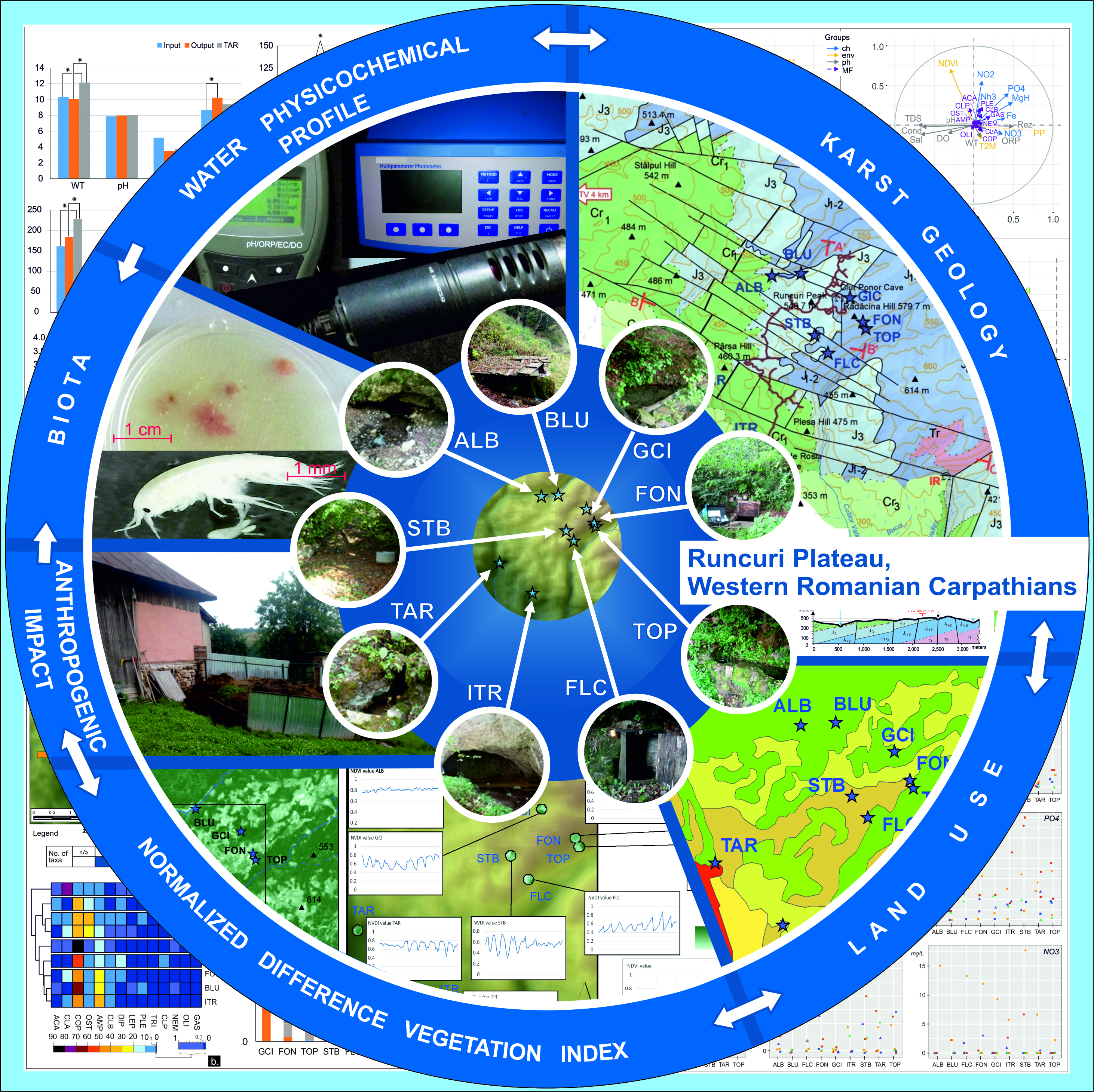
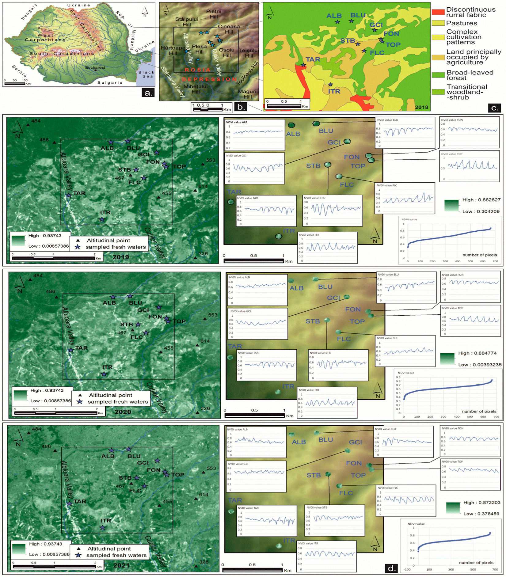
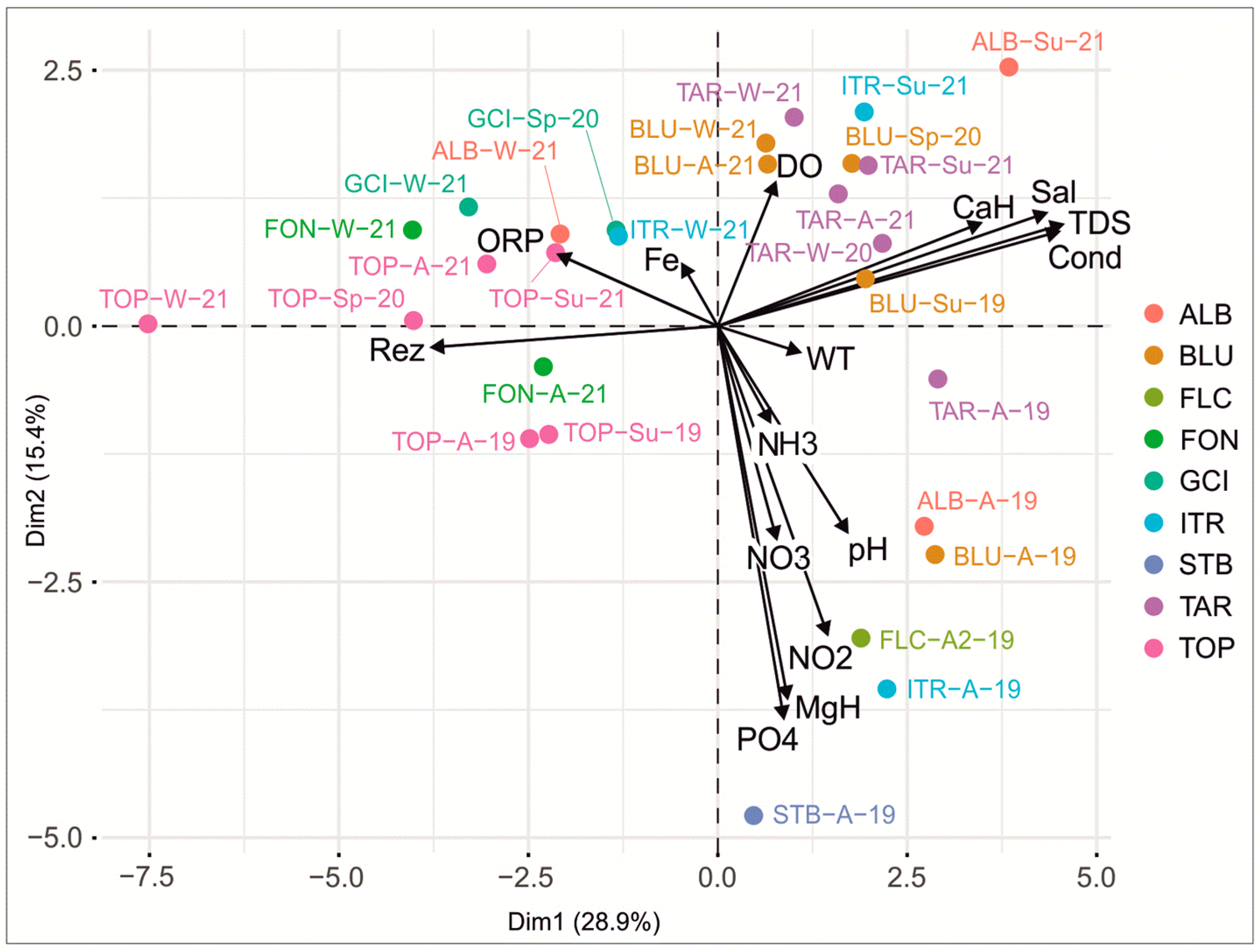
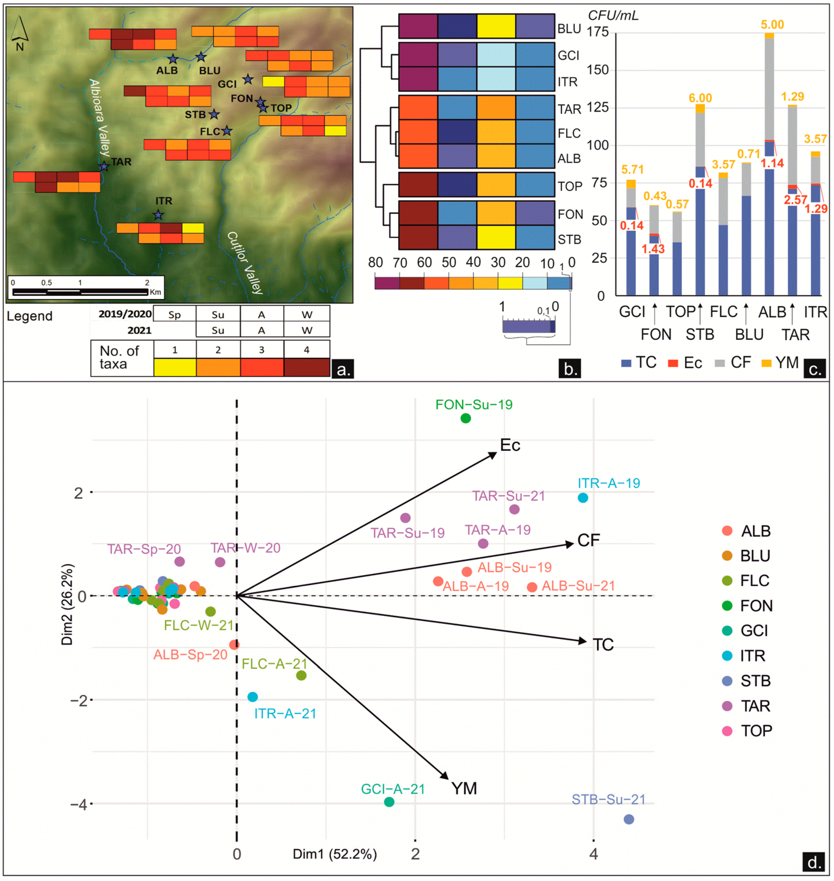
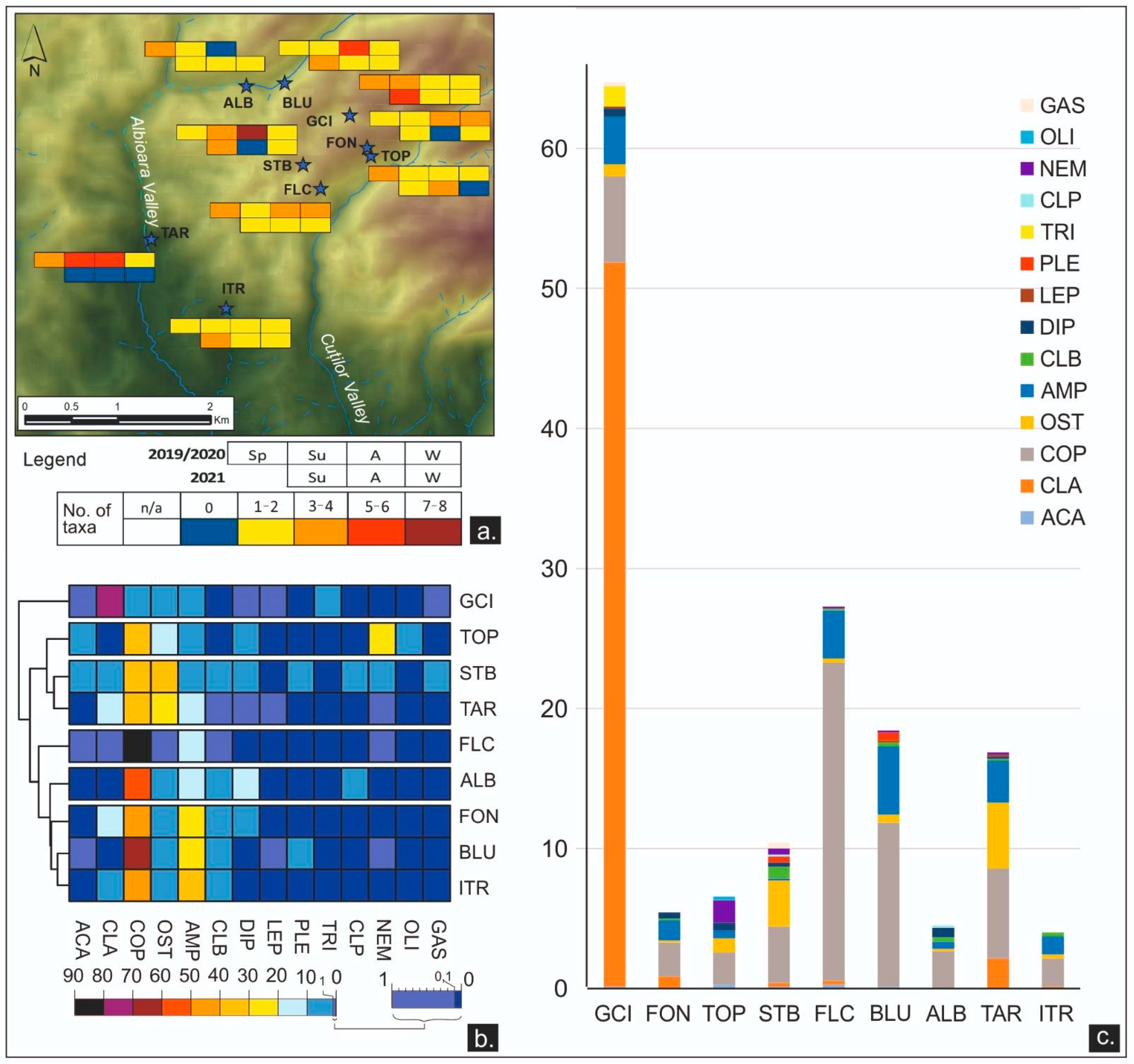
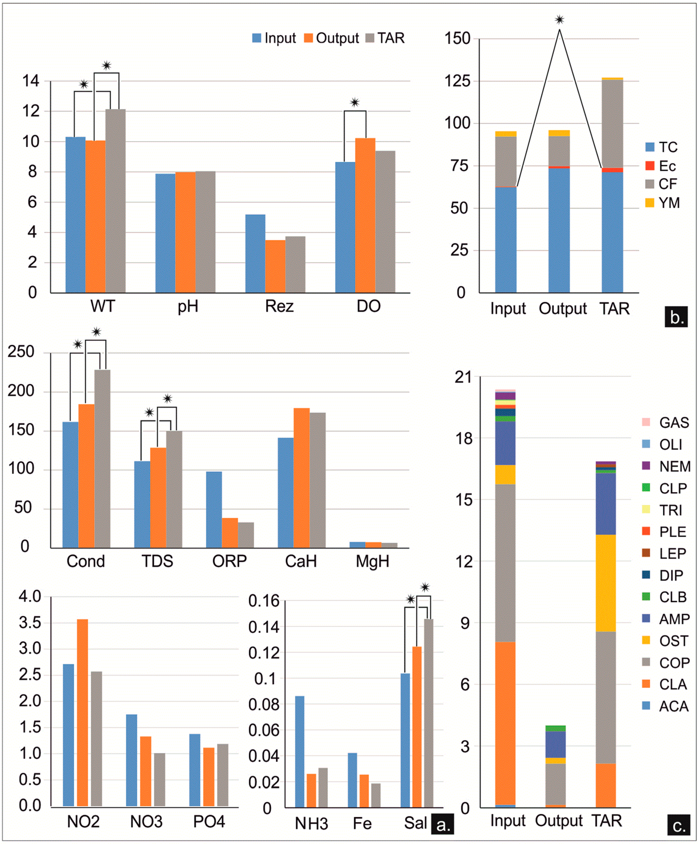
Table 1.
Description of the monitored springs. Input/output/independent output refers to the studied water sources within the hydrological context of the karst system of the Runcuri Plateau (KSRP). Age of rocks within which monitored springs developed: UJ1 = Upper part of the Lower Jurassic; J2–J3 = Limit of Middle and Upper Jurassic; J1, J2, J3 = Upper, Middle, and Lower Jurassic; C1 = Lower Cretaceous. Lithology: Lm = Limestones; Ma = Marls; Ss = Sandstones. Land use: Bf = Broad-leaved forest; Cc = Complex cultivation pattern; Pa = Land mainly used for agriculture; Ps = Pastures; Ws = Transitional woodland shrub; Rf = Discontinuous rural fabric. NDVI = Normalized difference vegetation index.
| Sampling Sites/Drinking Purpose | Water Type | Substrate | Hydrological Type | Age/ Lithology | Land Use | NDVI (Year/Index Value) | Altitude (m a.s.l.) |
|---|---|---|---|---|---|---|---|
| Groapa Ciur Izbuc (GCI)/occasionally used | Open-air Spring | Mud + Leaf | Input | UJ1/Lm | Bf | 2019/0.63 2020/0.66 2021/0.66 | 516 |
| La Foncea (FON)/ frequently used | Wood-covered Spring | Concrete dam + Ma | Input | UJ1/Ma | Cc, Pa, Bf | 2019/0.6 2020/0.66 2021/0.74 | 595 |
| La Topitori (TOP)/permanently used | Captured Spring | Concrete dam + Ss | Input | UJ1/Ss | Cc, Pa, Bf | 2019/0.61 2020/0.67 2021/0.66 | 580 |
| Știubei (STB)/permanently used | Open Well | Concrete tube + Mud | Input | J2-J3/Lm, Ma | Pa, Ws | 2019/0.56 2020/0.57 2021/0.75 | 531 |
| Fântâna lui Ciocan (FLC)/occasionally used | Wood-covered Spring | Lm + Mud | Input | UJ1/ Lm | Pa, Bf | 2019/0.54 2020/0.6 2021/0.67 | 503 |
| Izvorul Albastru (BLU)/occasionally used | Captured Spring | Concrete basin + Mud | Input | J2-J3/Lm, Ma | Bf | 2019/0.75 2020/0.59 2021/0.64 | 445 |
| Albioara (ALB)/ not used | Surface Stream | Mud + Gravel | Input | J1, J2, J3/ Ss, Lm, Ma | Bf | 2019/0.81 2020/0.66 2021/0.66 | 432 |
| Izvorul Țarina (TAR)/occasionally used | Open-air Spring | Sand + Lm | Independent output | C1/Lm | Bf, Pa, Rf | 2019/0.69 2020/0.66 2021/0.66 | 304 |
| Izbucul Toplița de Roșia (ITR)/permanently used | Cave stream resurgence | Gravel + Lm | Output | C1/Lm | Ws, Ps, Pa | 2019/0.62 2020/0.6 2021/0.59 | 290 |
Publisher’s Note: MDPI stays neutral with regard to jurisdictional claims in published maps and institutional affiliations. |
© 2022 by the authors. Licensee MDPI, Basel, Switzerland. This article is an open access article distributed under the terms and conditions of the Creative Commons Attribution (CC BY) license (https://creativecommons.org/licenses/by/4.0/).
Share and Cite
MDPI and ACS Style
Borda, D.R.; Cociuba, I.; Epure, L.; Cruceru, N.; Meleg, I.N. The Interplay of Environment and Biota in Assessing the Freshwater Quality in Karst. Diversity 2022, 14, 475. https://0-doi-org.brum.beds.ac.uk/10.3390/d14060475
AMA Style
Borda DR, Cociuba I, Epure L, Cruceru N, Meleg IN. The Interplay of Environment and Biota in Assessing the Freshwater Quality in Karst. Diversity. 2022; 14(6):475. https://0-doi-org.brum.beds.ac.uk/10.3390/d14060475
Chicago/Turabian StyleBorda, Daniela R., Ioan Cociuba, Laura Epure, Nicolae Cruceru, and Ioana N. Meleg. 2022. "The Interplay of Environment and Biota in Assessing the Freshwater Quality in Karst" Diversity 14, no. 6: 475. https://0-doi-org.brum.beds.ac.uk/10.3390/d14060475
Note that from the first issue of 2016, this journal uses article numbers instead of page numbers. See further details here.