
Location Detection and Tracking of Moving Targets by a 2D IR-UWB Radar System


Abstract
:
1. Introduction

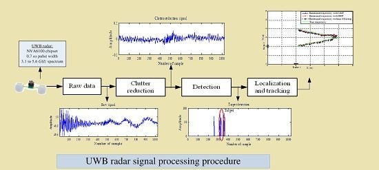
2. Signal Processing Steps for Moving-Target Detection, Localization and Tracking Using IR-UWB Radar
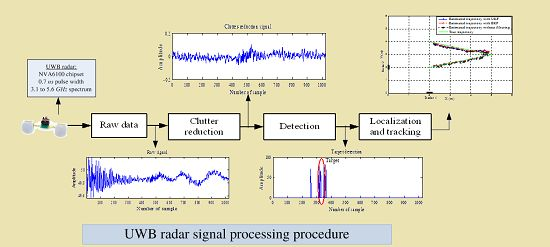
2.1. Clutter Reduction
2.1.1. Exponential Averaging Clutter-Reduction Method
2.1.2. Singular Value Decomposition Clutter-Reduction Method
2.1.3. Proposed KF-Based Clutter-Reduction Method
- -
- Time update:
- (1)
- Initial state and error covariance: , .
- (2)
- Project the state ahead: .
- (3)
- Project the error covariance ahead: .
- -
- Measurement update:
- (1)
- Compute the Kalman gain: .
- (2)
- Update the estimation with the measurement: .
- (3)
- Update the error covariance: .
- -
- Time update:
- (1)
- Initial state and error covariance: , .
- (2)
- Project the state ahead: .
- (3)
- Project the error covariance ahead: .
- -
- Measurement update:
- (1)
- Compute the Kalman gain: .
- (2)
- Update the estimate with the measurement: .
- (3)
- Update the error covariance: .
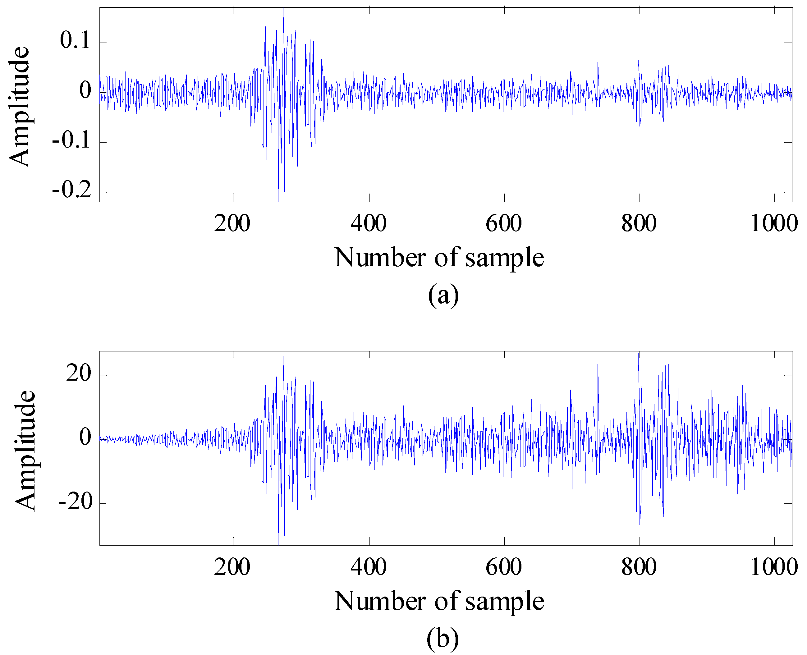
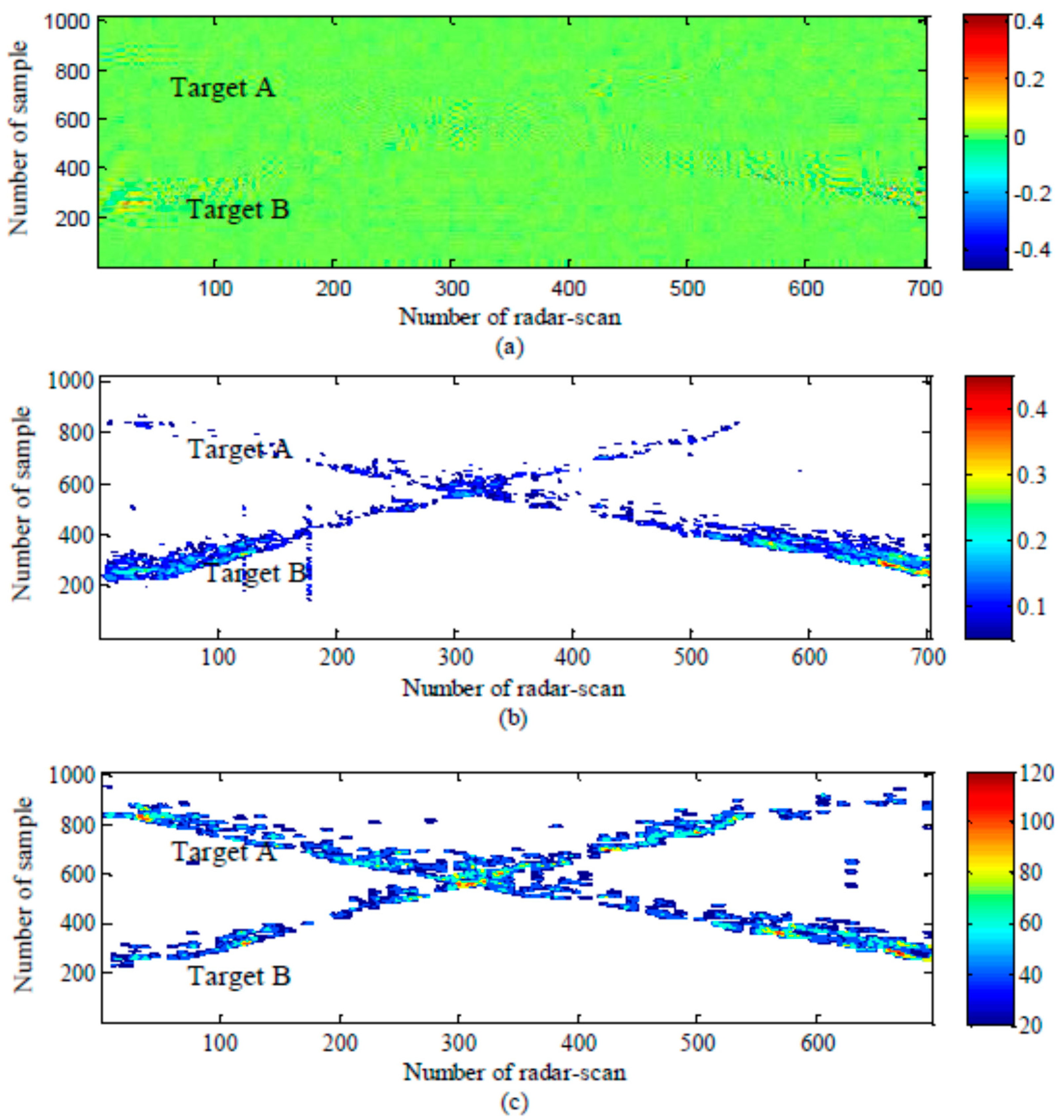
2.2. Detection
2.2.1. CLEAN Detection Algorithm

2.2.2. Modified CLEAN Detection Algorithm


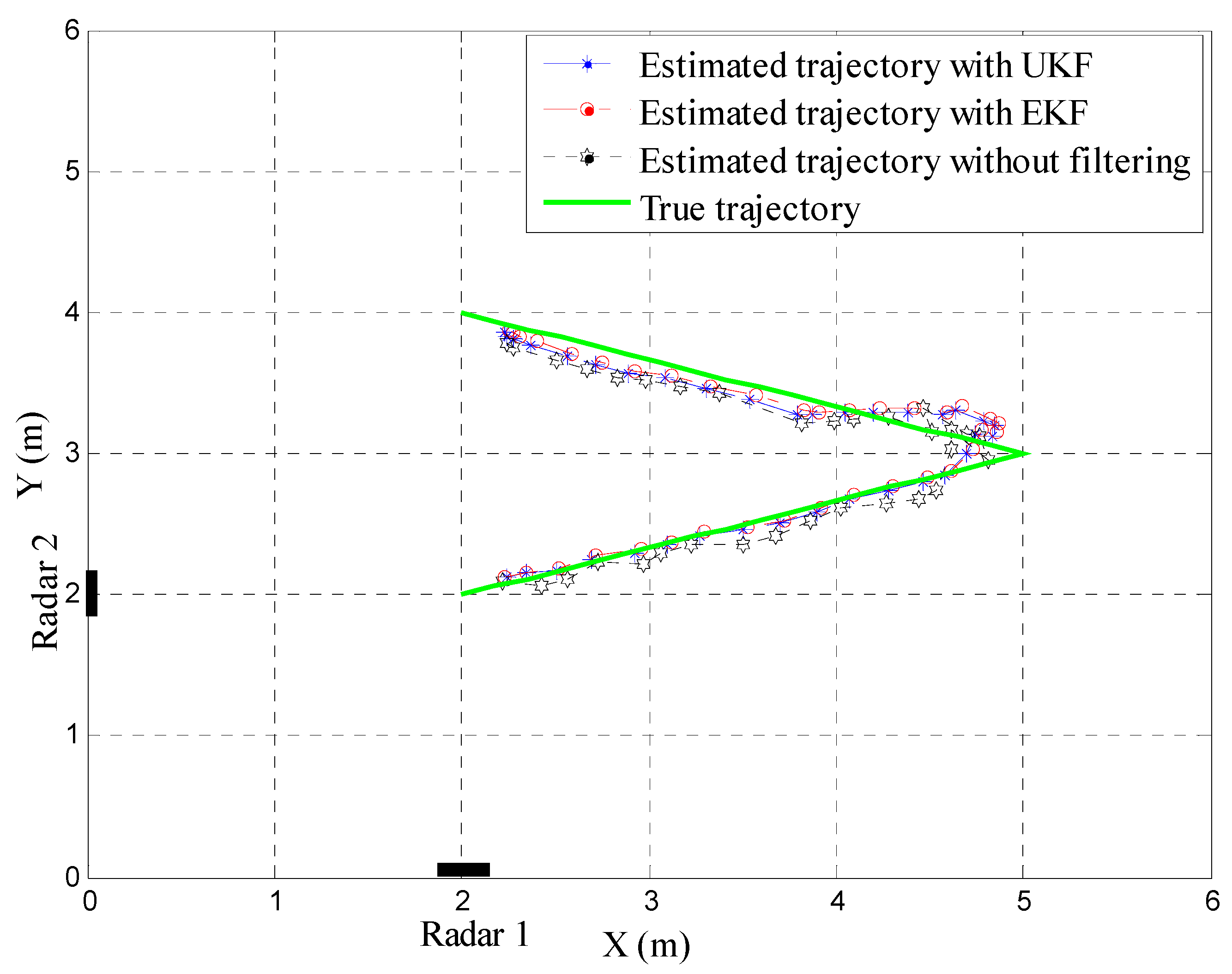
2.3. Localization and Tracking
2.3.1. Extended KF Localization and Tracking
- -
- Time update:
- (1)
- Initial state and error covariance: , .
- (2)
- Project the state ahead: .
- (3)
- Project the error covariance ahead: .
- -
- Measurement update:
- (1)
- Compute the measurement Jacobian matrix:
- (2)
- Compute the Kalman gain: .
- (3)
- Update the estimate with the measurement: ,where .
- (4)
- Update the error covariance: .
2.3.2. Unscented KF Localization and Tracking
- (1)
- Define three parameters to calculate the weight vector: .
- (2)
- Define the size of the state vector: .
- (3)
- Calculate the weight vector: .
- (4)
- Initial state and covariance: .
- (5)
- Calculate the sigma points: .
- -
- Time update
- (1)
- Propagate each sigma point through the state equation: .
- (2)
- Project the state ahead: .
- (3)
- Project the error covariance ahead: .
- -
- Measurement update
- (1)
- Propagate each sigma point through the measurement equation: , where .
- (2)
- Predict the measurement: .
- (3)
- Calculate the auto-covariance of the predicted measurement: .
- (4)
- Calculate the cross-covariance of the state and predicted measurements:.
- (5)
- Calculate the Kalman gain: .
- (6)
- Update the state estimate with the measurement: .
- (7)
- Update the error covariance: .
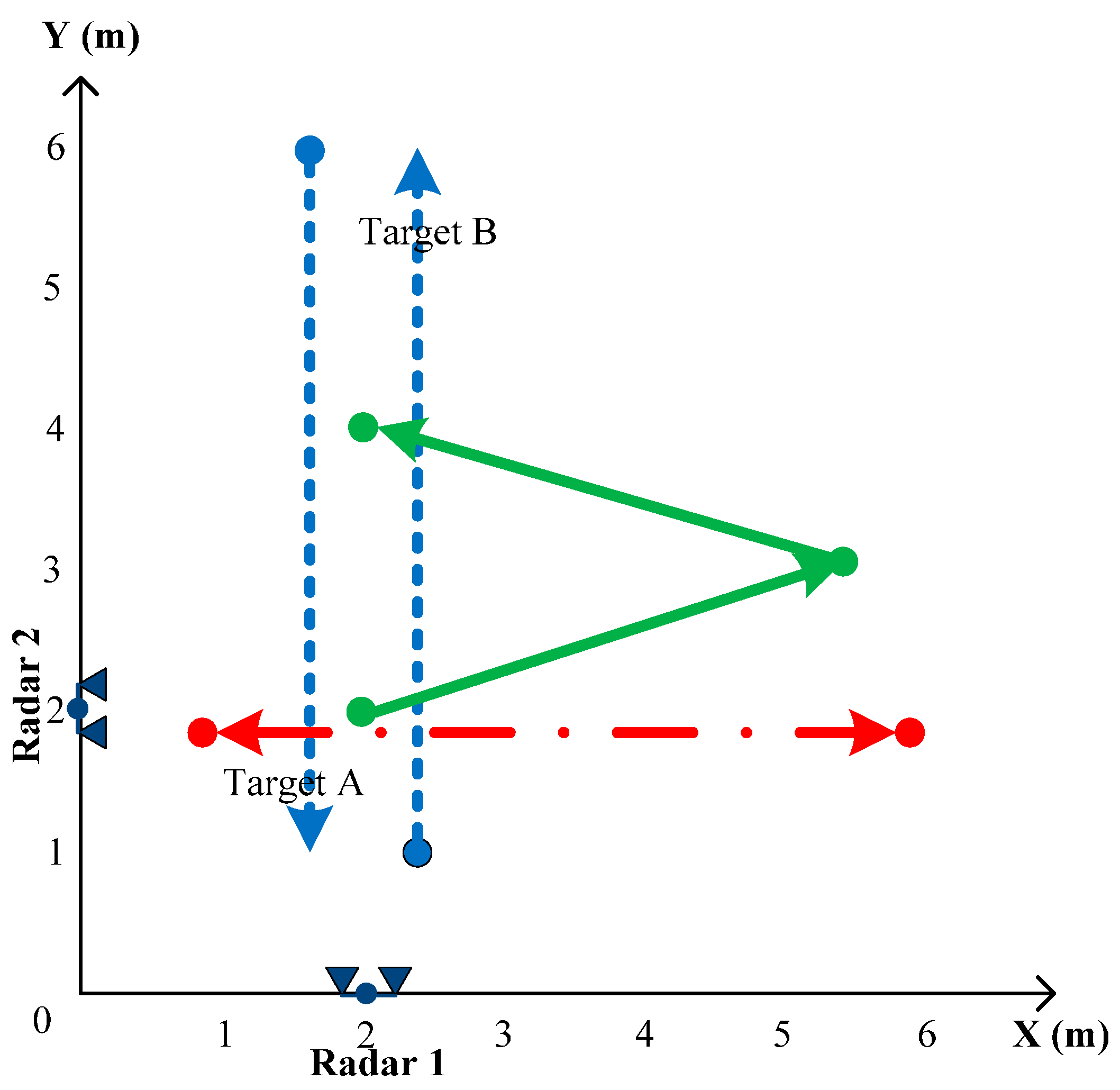
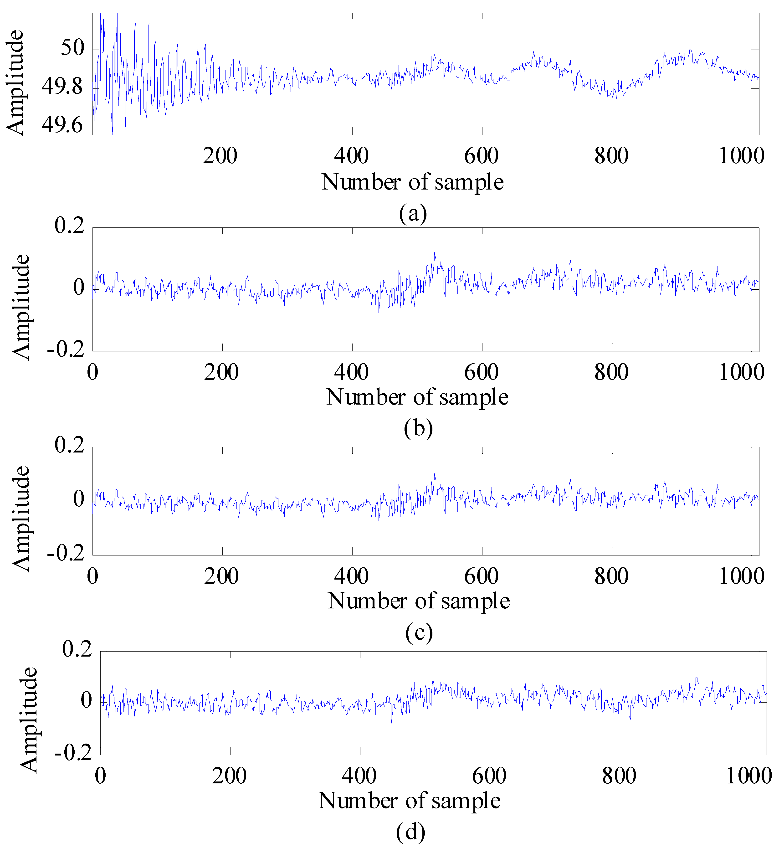
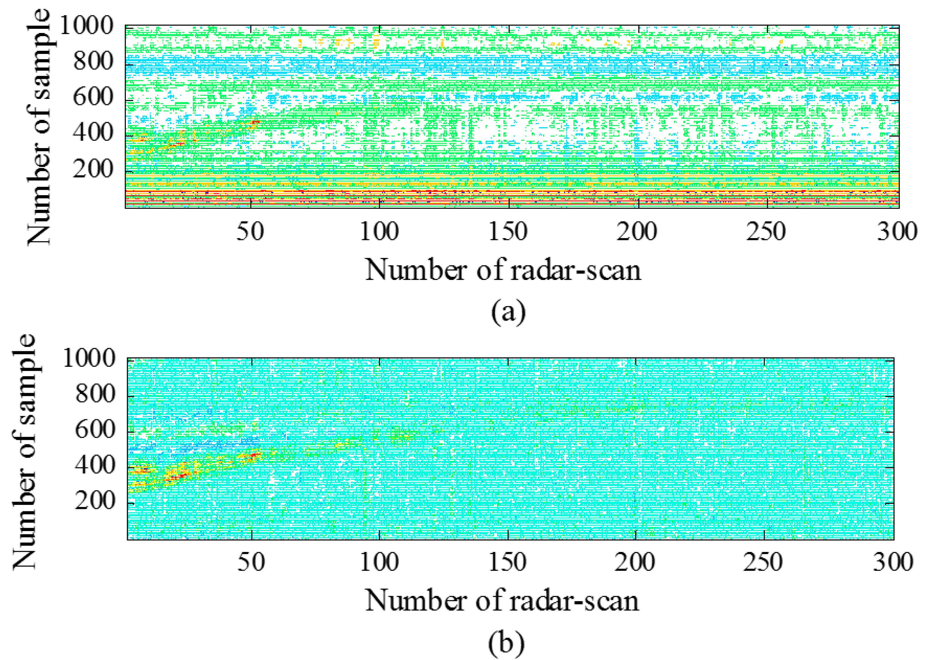
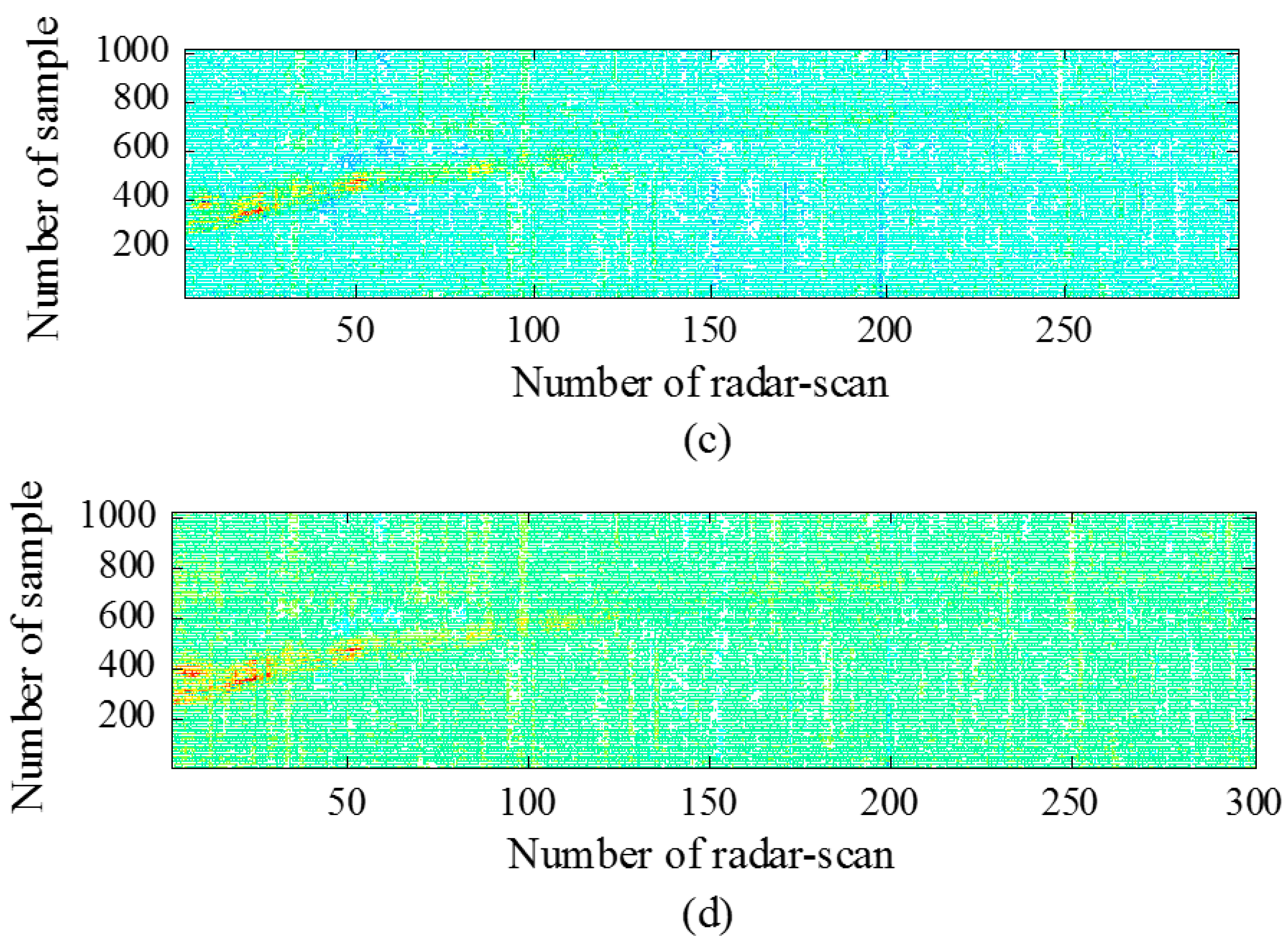
3. Experimental Results

| Conditions | Value |
|---|---|
| Pulse width | 0.7 ns |
| Number of sample in a frame | 1024 |
| Pulse repetition frequency (PRF) | 48 MHz |
| Frame range | Approximately 2 m (in 48 MHz·PRF) |

| Parameters | Value |
|---|---|
| Exponential factor in EA method | α = 0.95 |
| Compensated vector in modified CLEAN algorithm | α[n] = [1,2,...1024] for n = 1, 2, ..., 1024 |
| Threshold in modified CLEAN algorithm | T = 3 × mean of compensated-radar-scan signals |
| 2D window size | 10 samples × 10 radar scans |

| Clutter-Reduction Method | Average RMSE |
|---|---|
| Kalman Filter | 0.1029 |
| Exponential Average | 0.2031 |
| Singular Value Decomposition | 0.1342 |


| Detection Method | Detection Rate | |
|---|---|---|
| Target A | Target B | |
| Conventional CLEAN method | 45% | 55% |
| Modified CLEAN method | 73% | 87% |


| Tracking | RMSE (m) |
|---|---|
| Estimated trajectory without filtering | 0.2478 |
| Estimated trajectory by EKF | 0.2373 |
| Estimated trajectory by UKF | 0.2260 |
4. Conclusions
Acknowledgments
Author Contributions
Conflicts of Interest
References
- Patwari, N.; Ash, J.N.; Kyperountas, S.; Hero, A.O.; Moses, R.L.; Correal, N.S. Locating the nodes: Cooperative localization in wireless sensor network. IEEE Signal Process. Mag. 2005, 22, 54–69. [Google Scholar] [CrossRef]
- Decarli, N.; Guidi, F.; Dardari, D. A Novel Joint RFID and Radar Sensor Network for Passive Localization: Design and Performance Bounds. IEEE J. Sel. Top. Signal Process. 2014, 8, 80–95. [Google Scholar] [CrossRef]
- Fontana, R.J. Recent system applications of short-pulse ultra-wideband (UWB) technology. IEEE Trans. Microw. Theory Tech. 2004, 52, 2087–2104. [Google Scholar] [CrossRef]
- Hashemi, H. Impulse Response Modeling of Indoor Radio Propagation Channels. IEEE J. Sel. Areas Commun. 1993, 11, 967–978. [Google Scholar] [CrossRef]
- Sahinoglu, Z.; Gezici, S.; Guvenc, I. Ultra-Wideband Positioning Systems: Theoretical Limits, Ranging Algorithms, and Protocols, 1st ed.; Cambridge University Press: Cambridge, UK, 2008. [Google Scholar]
- Rovnakova, J.; Svecova, M.; Nguyen, T.T.; Sachs, J. Signal Processing for through Wall Moving Target Tracking by M-Sequence UWB Radar. In Proceedings of the 18th International Conference Radioelektronika, Prague, Czech, 1–4 April 2008.
- Cristani, M.; Farenzena, M.; Bloisiand, D.; Murino, V. Background Subtraction for Automated Multisensor Surveillance: A Comprehensive Review. Eurasip J. Adv. Signal Process. 2010. [Google Scholar] [CrossRef]
- Abujarad, F.; Jostingmeier, A.; Omar, A.S. Clutter Removal for Landmine using Different Signal Processing Technique. In Proceedings of Tenth International Conference on Ground Penetrating Radar, Delft, The Netherlands; 2004; pp. 697–700. [Google Scholar]
- Zhao, X.W.; Gaugue, A.; Lièbe, C.; Khamlichi, J.; Menard, M. Through the wall detection and localization of a moving target with a bistatic UWB radar system. In Proceedings of the 2010 European Radar Conference (EuRAD), Paris, France, 30 September–1 October 2010; pp. 204–207.
- Zetik, R.; Crabble, S.; Krajnak, J.; Perl, P.; Sachs, J.; Thoma, R.S. Detection and localization of persons behind obstacles using M-sequence through-the-wall radar. In Proceedings of Sensors, and Command, Control, Communications, and Intelligence (C3I) Technologies for Homeland Security and Homeland Defense V, FL, USA, 10 May 2006.
- Singh, S.; Liang, Q.L.; Chen, D.C.; Sheng, L. Sense through wall human detection using UWB radar. Eurasip J. Wirel. Commun. Netw. 2011, 2011, 20. [Google Scholar] [CrossRef]
- Verma, P.K.; Gaikwad, A.N.; Singh, D.; Nigam, M.J. Analysis of Clutter Reduction Techniques for Through the Wall Imaging in UWB Range. Progr. Electromagn. Res. B 2009, 17, 29–48. [Google Scholar] [CrossRef]
- Immoreev, I.I. Features Detection in UWB Radar Signals. In Ultra-Wideband Radar Technology, 1st ed.; Taylor, J.D., Ed.; CRC Press: Boca Raton, FL, USA, 2001. [Google Scholar]
- Liang, Q.; Zhang, B.; Wu, X. UWB Radar for Target Detection: DCT Versus Matched Filter Approaches. In Proceedings of 2012 IEEE Globecom Workshops, Anaheim, CA, USA, 3–7 December 2012; pp. 1435–1439.
- Kocur, D.; Gamec, J.; Svecova, M.; Gamcova, M.; Rovnakova, J. Imaging Method: An Efficient Algorithm for Moving Target Tracking by UWB Radar. Acta Polytech. Hung. 2010, 7, 5–24. [Google Scholar]
- Chang, S.; Sharan, R.; Wolf, M.; Mitsumoto, N.; Burdick, J. People Tracking with UWB Radar Using a Multiple-Hypothesis Tracking of Clusters (MHTC) Method. Int. J. Social Robot. 2010, 2, 3–18. [Google Scholar] [CrossRef]
- Gezici, S.; Zhi, T.; Giannakis, G.B.; Kobayashi, H.; Molisch, A.F.; Poor, H.V.; Sahinoglu, Z. Localization via ultra-wideband radios: A look at positioning aspects for future sensor networks. IEEE Signal Process. Mag. 2005, 2, 70–84. [Google Scholar] [CrossRef]
- Švecová, M.; Kocur, D.; Zetik, R.; Rovnakova, J. Target localization by a multistatic UWB radar. In Proceedings of International Conference Radioelektronika (RADIOELEKTRONIKA), Brno, Czech, 19–21 April 2010; pp. 1–4.
- Park, J.S.; Baek, I.S.; Cho, S.H. Localizations of multiple targets using multistatic UWB radar systems, In Proceedings of IEEE International Conference on Network Infrastructure and Digital Content (IC-NIDC). In Proceedings of IEEE International Conference on Network Infrastructure and Digital Content (IC-NIDC), Beijing, China, 21–23 September 2012; pp. 586–590.
- He, Y.; Savelyev, T.; Yarovoy, A. Two-stage algorithm for extended target tracking by multistatic UWB radar. In Proceedings of IEEE CIE International Conference on Radar, Chengdu, China, 24–27 October 2011; pp. 795–799.
- Sobhani, B.; Mazzotti, M.; Paolini, E.; Giorgetti, A.; Chiani, M. Multiple target detection and localization in UWB multistatic radars. In Proceedings of IEEE International Conference on Ultra-Wideband (ICUWB), Paris, France, 1–3 September 2014; pp. 135–140.
- Giorgetti, A.; Chiani, M. Time-of-Arrival Estimation Based on Information Theoretic Criteria. IEEE Trans. Signal Process. 2013, 61, 1869–1879. [Google Scholar] [CrossRef]
- Paolini, E.; Giorgetti, A.; Chiani, M.; Minutolo, R.; Montanari, M. Localization capability of cooperative anti-intruder radar systems. Eurasip J. Adv. Signal Process. 2008, 2008, 1–14. [Google Scholar] [CrossRef]
- Kocur, D.; Svecová, M.; Rovňáková, J. Through-the-wall localization of a moving target by two independent ultra wideband (UWB) radar systems. Sensors 2013, 13, 11969–11997. [Google Scholar] [CrossRef] [PubMed]
- Sobhani, B.; Paolini, E.; Giorgetti, A.; Mazzotti, M.; Chiani, M. Target Tracking for UWB Multistatic Radar Sensor Networks. IEEE J. Sel. Top. Signal Process. 2014, 8, 125–136. [Google Scholar] [CrossRef]
- Bartoletti, S.; Conti, A.; Giorgetti, A.; Win, M.Z. Sensor Radar Networks for Indoor Tracking. IEEE Wirel. Comm. Lett. 2014, 1, 157–160. [Google Scholar]
- Sobhani, B.; Mazzotti, M.; Paolini, E.; Giorgetti, A.; Chiani, M. Effect of State Space Partitioning on Bayesian Tracking for UWB Radar Sensor Networks. In Proceedings of IEEE International Conference on Ultra-Wideband (ICUWB), Sydney, Australia, 15–18 September 2013; pp. 120–125.
- Chiani, M.; Giorgetti, A.; Mazzotti, M.; Minutolo, R.; Paolini, E. Target Detection Metrics and Tracking for UWB Radar Sensor Networks. In Proceedings of IEEE International Conference on Ultra-Wideband (ICUWB), Vancouver, Canada, 9–11 September 2009; pp. 469–474.
- Nguyen, V.H.; Kim, D.-M.; Kwon, G.-R.; Pyun, J.-Y. Clutter Reduction on Impulse Radio Ultra Wideband Radar Signal. In Proceedings of International Technical Conference on Circuit/Systems Computers and Communications (ITC-CSCC), Yeosu, Korea, 30 June–3 July 2013; pp. 1091–1094.
- Nguyen, V.H.; Pyun, J.-Y. Improved Target Detection for Moving Object in IR-UWB Radar. In Proceedings of the International Conference on Green and Human Information Technology, Ho Chi Minh City, Vietnam, 12–14 February 2014; pp. 69–73.
- Brown, R.G.; Hwang, P.Y.C. Introduction to Random Signals and Applied Kalman Filtering, 3rd ed.; John Wiley & Sons, INC: New York, NY, USA, 1996. [Google Scholar]
- Irahhauten, Z.; Nikookar, H.; Janssen, G.J.M. An overview of ultra wide band indoor channel measurements and modeling. IEEE Microw. Wirel. Compon. Lett. 2004, 14, 386–388. [Google Scholar] [CrossRef]
- Chui, C.K.; Chen, G. Extended Kalman Filter and System Identification. In Kalman Filtering with Real-Time Applications, 4th ed.; Springer: Berlin, Germany, 2009; pp. 108–129. [Google Scholar]
- Welch, G.; Bishop, G. An Introduction to the Kalman Filter. Department of Computer Science, University of North California: Chapel Hill, NC, USA, 2006. [Google Scholar]
- Julier, S.J.; Uhlmann, J.K. A New Extension of the Kalman Filter to Nonlinear Systems. In Proceedings of the AeroSense: 11th International Symposium Aerospace/Defense Sensing, Simulation and Controls, Orlando, FL, USA, 21 April 1997; pp. 182–193.
- Julier, S.J.; Uhlmann, J.K. Unscented Filtering and Nonlinear Estimation. Proc. IEEE 2004, 92, 401–422. [Google Scholar] [CrossRef]
- Taylor, J.D.; Wisland, D.T. Novelda Nanoscale Impulse Radar. In Ultra-wideband Radar: Applications and Design, 1st ed.; Taylor, J.D., Ed.; CRC Press: New York, NY, USA, 2012; pp. 373–388. [Google Scholar]
© 2015 by the authors; licensee MDPI, Basel, Switzerland. This article is an open access article distributed under the terms and conditions of the Creative Commons Attribution license (http://creativecommons.org/licenses/by/4.0/).
Share and Cite
Nguyen, V.-H.; Pyun, J.-Y. Location Detection and Tracking of Moving Targets by a 2D IR-UWB Radar System. Sensors 2015, 15, 6740-6762. https://0-doi-org.brum.beds.ac.uk/10.3390/s150306740
Nguyen V-H, Pyun J-Y. Location Detection and Tracking of Moving Targets by a 2D IR-UWB Radar System. Sensors. 2015; 15(3):6740-6762. https://0-doi-org.brum.beds.ac.uk/10.3390/s150306740
Chicago/Turabian StyleNguyen, Van-Han, and Jae-Young Pyun. 2015. "Location Detection and Tracking of Moving Targets by a 2D IR-UWB Radar System" Sensors 15, no. 3: 6740-6762. https://0-doi-org.brum.beds.ac.uk/10.3390/s150306740