
A New Method of Using Sensor Arrays for Gas Leakage Location Based on Correlation of the Time-Space Domain of Continuous Ultrasound

Abstract
:1. Introduction
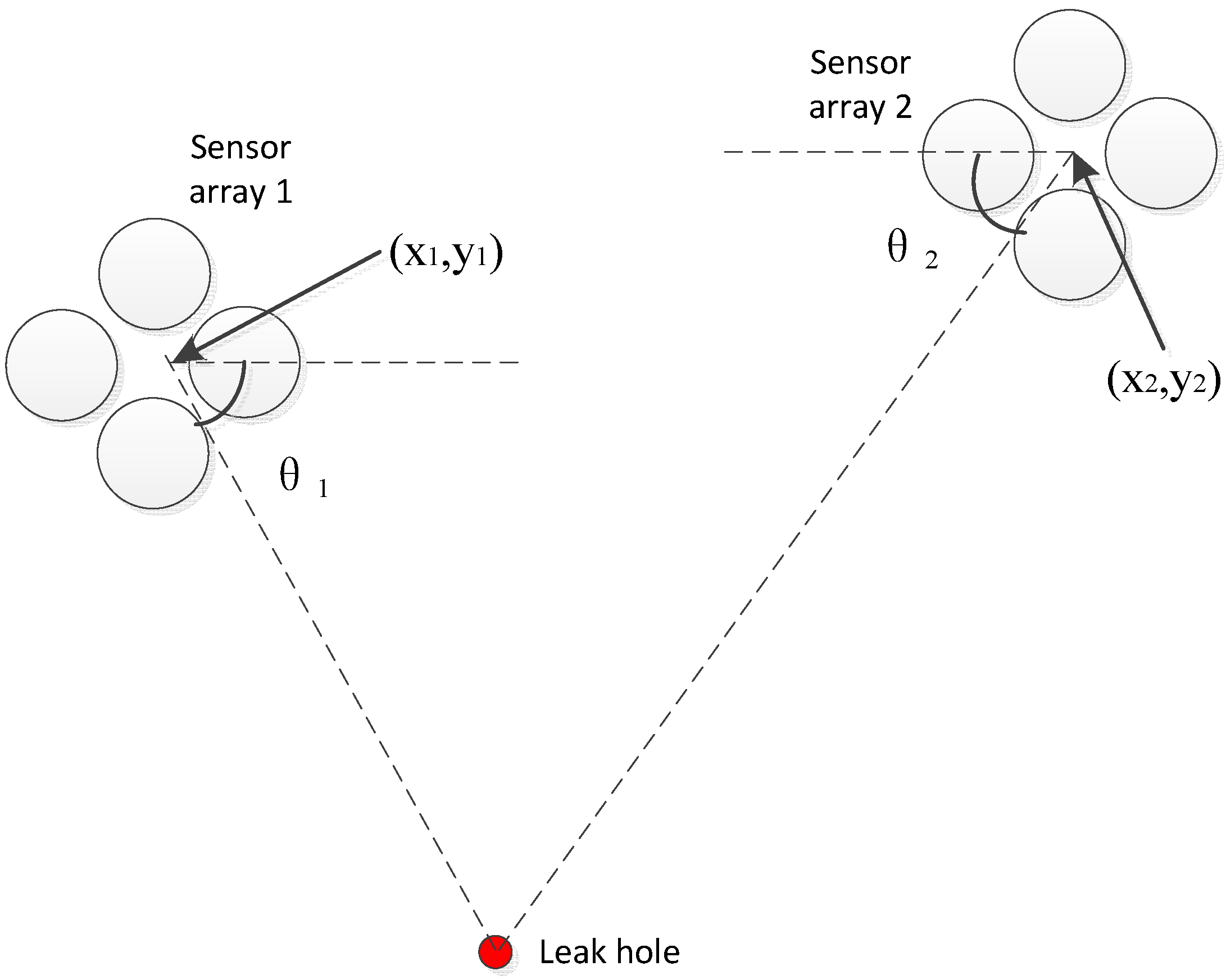
2. Location Method

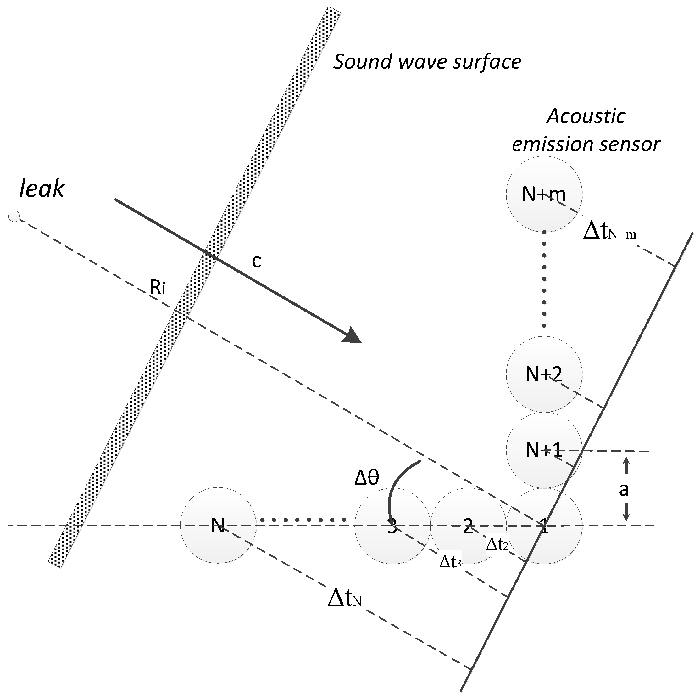
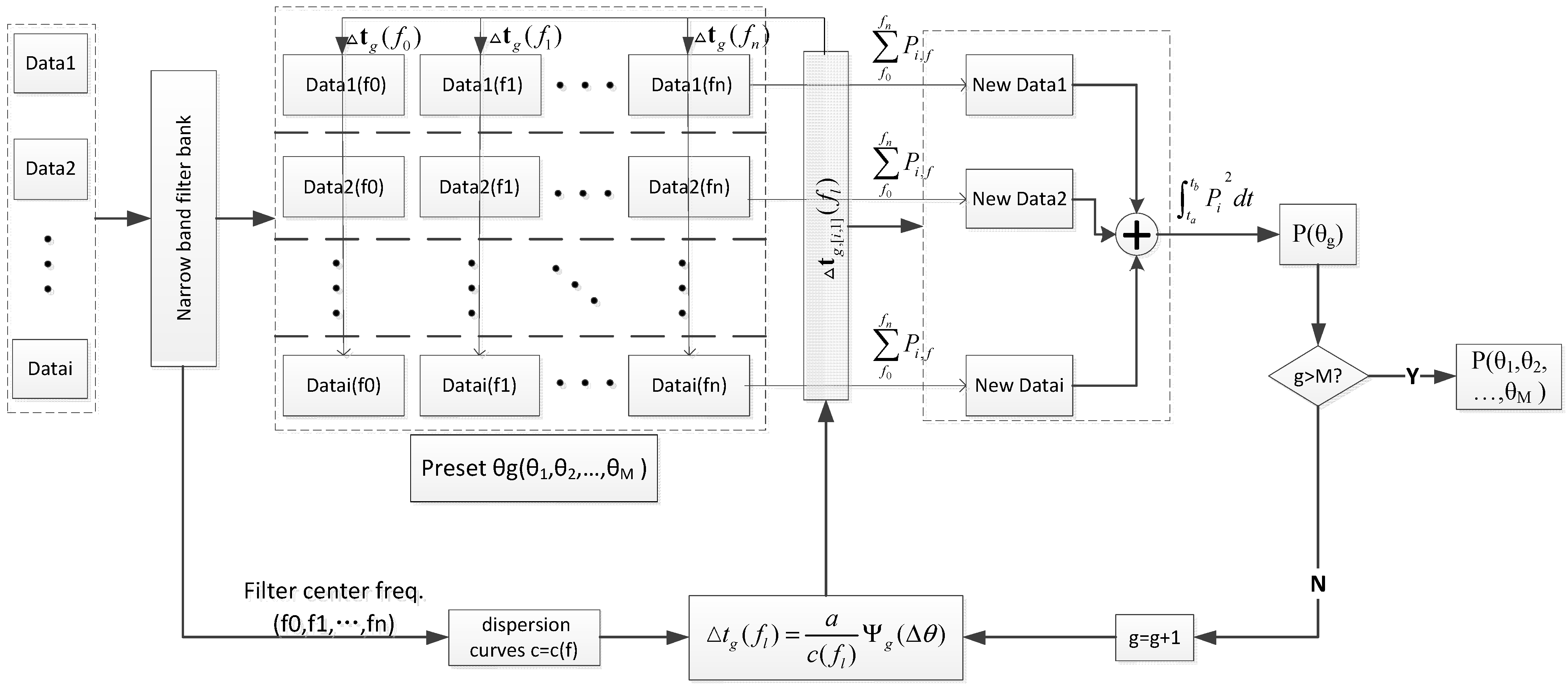
3. Algorithm Theory


4. Experimental Setup
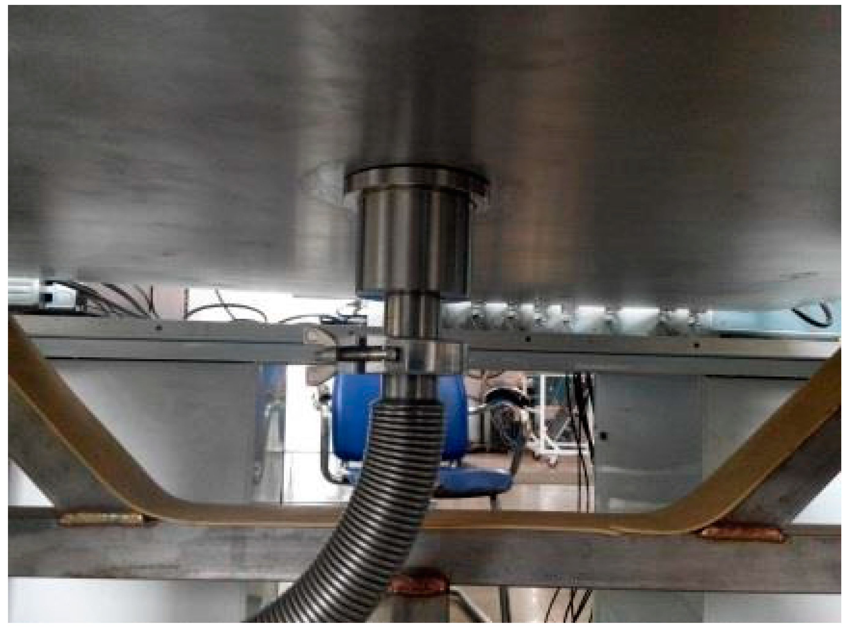
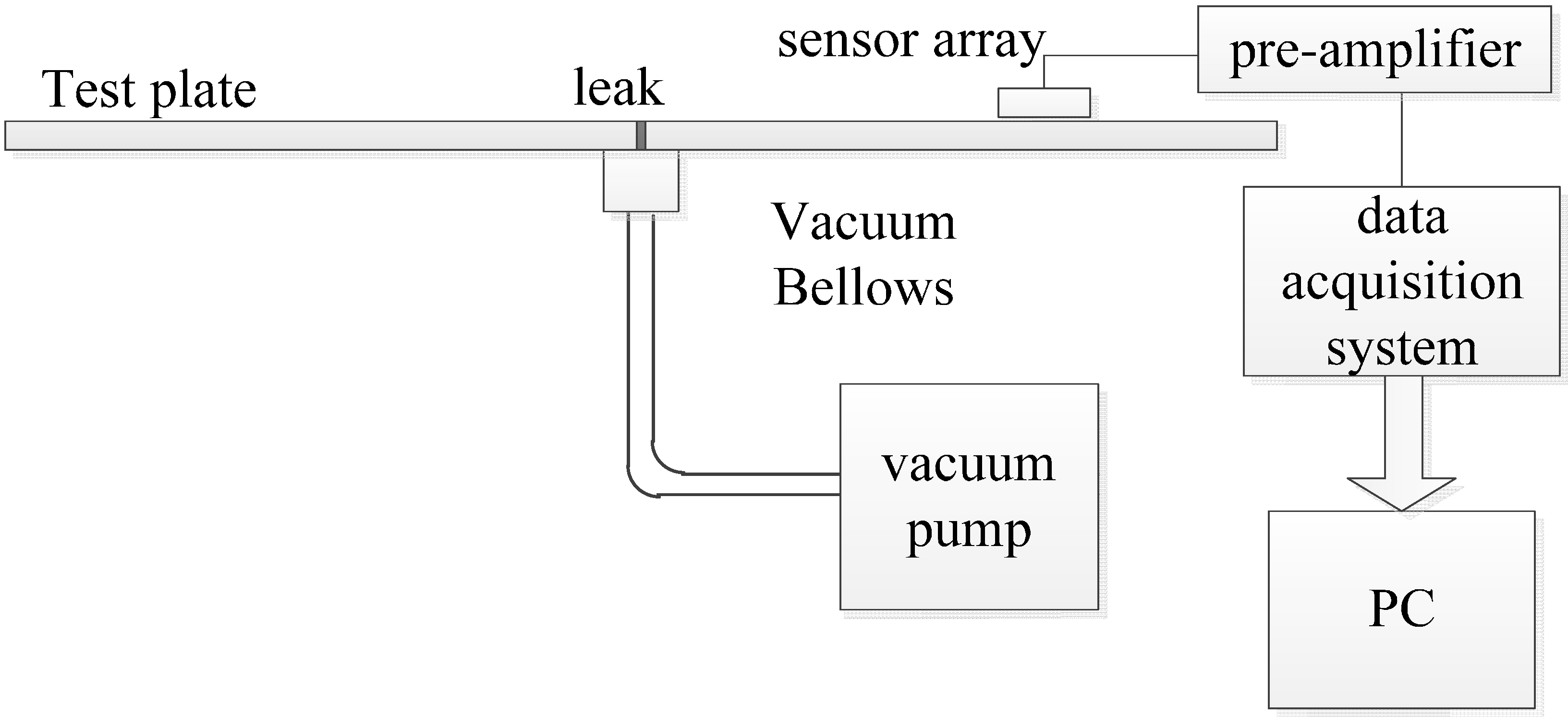
4.1. Assembly of the Apparatus


| Material | Modulus of Elasticity E (KN/mm2) | Poisson’s Ratio σ | Density ρ (g·cm−3) |
|---|---|---|---|
| 302 Stainless steel | 210 | 0.305 | 7.93 |
| Magnesium aluminum alloy | 40 | 0.275 | <1.8 |

| Mode Used | 302 Steel | Magnesium Aluminum Alloy | ||
|---|---|---|---|---|
| Mean Error (°) | Variance | Mean Error (°) | Variance | |
| A0 mode | 0.29 | 1.9039 | 0.1925 | 1.252178 |
| S0 mode | 6.04 | 388.8854 | 11.7425 | 700.4788 |
| A0&S0 mode | 0.28 | 3.1546 | 0.54 | 3.206737 |
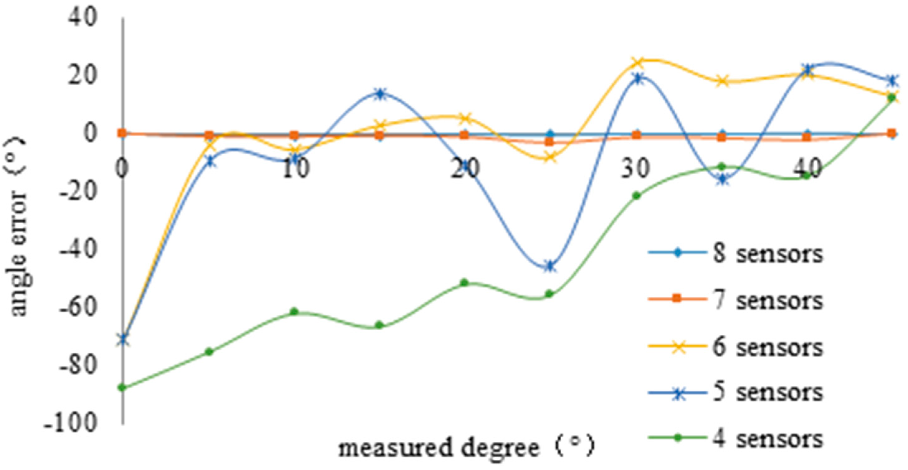
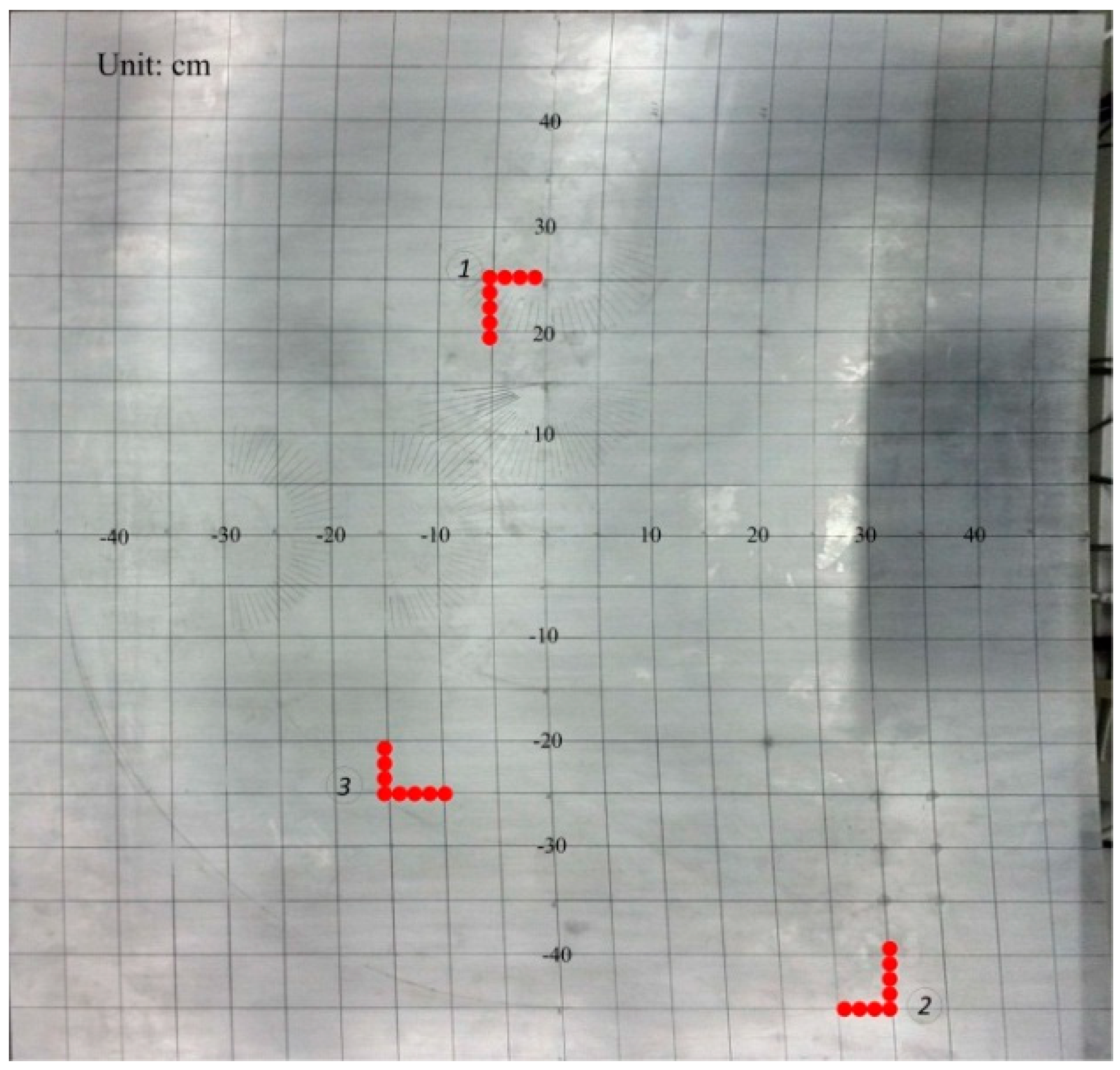
4.2. Sizing of the Array

| Item | Value |
|---|---|
| Peak Sensitivity, Ref V/(m/s) | 62 dB |
| Peak Sensitivity, Ref V/μbar | −72 dB |
| Operating Frequency Range | 125–750 kHz |
| Resonant Frequency, Ref V/(m/s) | 140 kHz |
| Resonant Frequency, Ref V/μbar | 300 kHz |
| Directionality | ± 1.5 dB |
| Diameter | 8 mm |

5. Results and Discussion


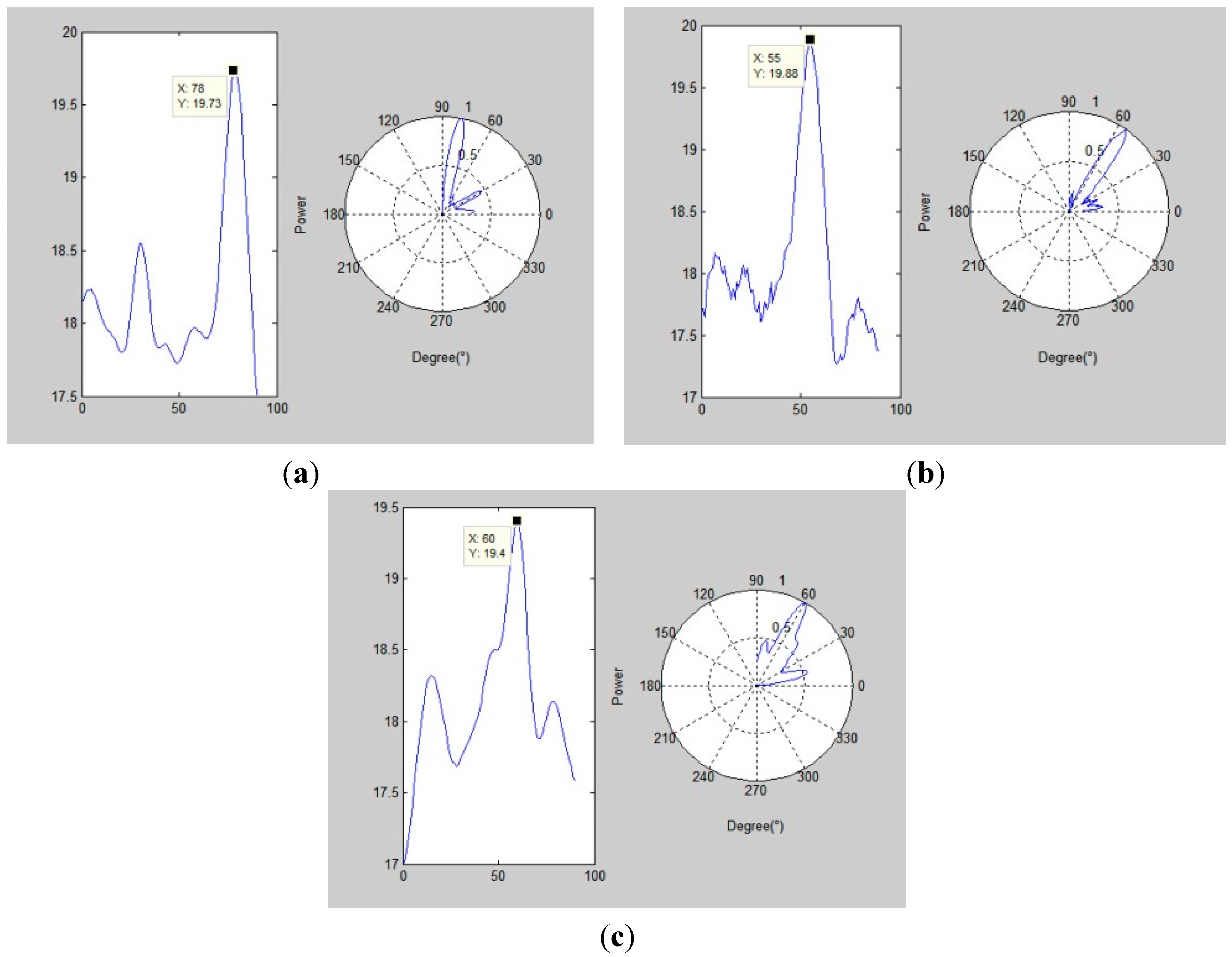
| Actual Leakage Angle (°) | Proposed Method without the Sound Velocity’s Changing (c = 2000 m/s) | Proposed Method | |||
|---|---|---|---|---|---|
| Mean Error (°) | Variance | Mean Error (°) | Variance | ||
| No.1 array | 78.7 | 5.7 | 208.01 | 0 | 3.38 |
| No.2 array | 56.3 | 19.3 | 179.25 | 0.4 | 2.96 |
| No.3 array | 60 | −13.1 | 152.77 | −0.1 | 3.19 |
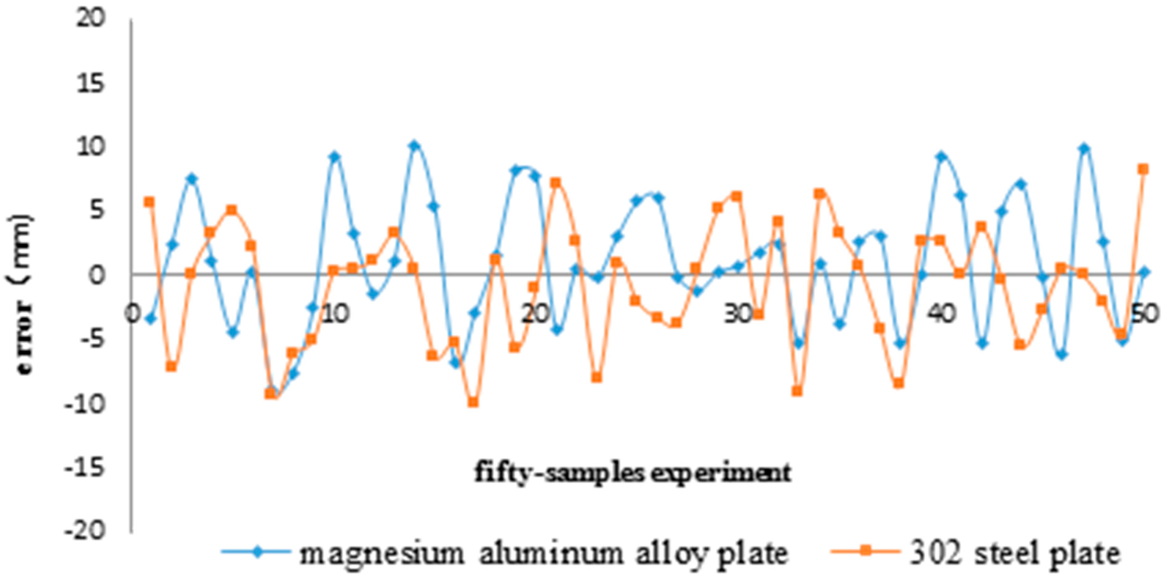
| The Coordinate of Leakage Point(mm) | The Coordinate of Estimate Leakage Point (mm) | Error d (mm) | |
|---|---|---|---|
| No.1 and No.2 array | (0,0) | (1.89,−9.67) | 9.85 |
| No.1 and No.3 array | (0,0) | (−1.64,8.00) | 8.17 |
| No.2 and No.3 array | (0,0) | (−5.51,1.22) | 5.64 |
| Comprehensive result | (0,0) | (−5.26,−0.45) | 5.28 |


6. Conclusions
- (1)
- Experimental tests show that the leakage-generated acoustic emission signal is influenced by some factors such as media characteristics, leakage hole size, and sensor response. Moreover, the distortion which is introduced by the sensors cannot be neglected in order to achieve higher location accuracy.
- (2)
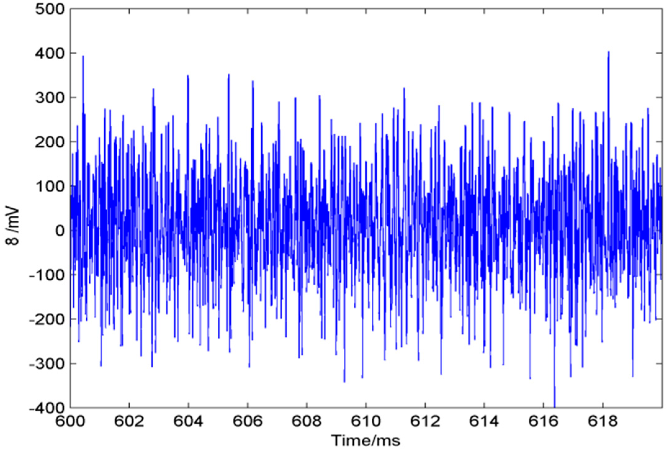
- The leakage ultrasonic signal is a noise-like continuous broadband signal. According to the experimental results, the signal collected by an AE sensor is mainly in A0 mode (plate is less than 6 mm thick, and signal frequency within the range 100–300 kHz). Meanwhile, the S0 mode has an extremely small influence on the locating result, thus S0 can be neglected.
- (3)
- This research presents a high-accuracy leakage source location method using fewer sensors to compose the sensor array. Moreover, the study solves the gas continuous leakage real-time localization problem based on the correlation of the signal in the time-space domain, which is generated from the leakage hole. Experimental results show that when the size of plate is 1000 × 1000 × 2.5 mm and the diameter of the leakage hole is larger than 0.8 mm, the mean location error is 5.83 mm, and the maximum location error is generally less than 10 mm. These results are typical of many others we have obtained. Therefore, this method provides a new approach to successfully solve the problem of real-time detection of gas leakages and location in large pressure vessels.
Acknowledgments
Author Contributions
Conflicts of Interest
References
- Murvay, P.S.; Silea, I. A Survey on Gas Leak Detection and Localization Techniques. J. Loss Prevent. Process Ind. 2012, 25, 966–973. [Google Scholar] [CrossRef]
- Gaunce, M.T.; Thompson, D.R. Mir Photo/TV Survey (DTO-1118): STS-86 Mission Report; JSC-28194; NASA: Washington, DC, USA, 1997; pp. 18–19.
- Graf, J.C.; Kittrell, C.; Arepalli, S. Mir Leak Detection Using Fluorescent Tracer Gases. SAE Tech. Pap. 1999. [Google Scholar] [CrossRef]
- Kroll, A.; Baetz, W.; Peretzki, D. On Autonomous Detection of Pressured Air and Gas Leaks Using Passive IR-Thermography for Mobile Robot Application. In Proceedings of the IEEE International Conference on Robotics and Automation, Kobe, Japan, 12–17 May 2009; pp. 921–926.
- Lemon, D.K.; Friesel, M.A.; Griffin, J.W.; Skorpik, J.R.; Shepard, C.L.; Antoniak, Z.I.; Kurtz, R.J. Technology Evaluation for Space Station Atmospheric Leakage; Report Number PNL-7269; Pacific Northwest Lab.: Richland, WA, USA, 1990.
- Fukushige, S.; Akahoshi, Y.; Koura, T.; Harada, S. Development of perforation hole detection system for space debris impact. Int. J. Impact Eng. 2006, 33, 273–284. [Google Scholar] [CrossRef]
- Al-Nasser, Y.N.; Datta, S.K.; Shah, A.H. Scattering of Lamb waves by a normal rectangular strip weldment. Ultrasonics 1991, 29, 125–132. [Google Scholar] [CrossRef]
- Greve, D.W.; Tyson, N; Oppenheim, I.J. Interaction of defects with Lamb waves in complex geometries. In Proceedings of the 2005 IEEE Ultrasonics Symposium, Rotterdam, Netherlands, 18–21 September 2005; pp. 297–300.
- Ziola, S.M.; Gorman, M.R. Source location in thin plates using cross-correlation. J. Acoust. Soc. Am. 1991, 90, 2551–2556. [Google Scholar] [CrossRef]
- Beigelbeck, R.; Antlinger, H.; Cerimovic, S.; Clara, S.; Keplinger, F.; Jakoby, B. Resonant pressure wave setup for simultaneous sensing of longitudinal viscosity and sound velocity of liquids. Meas. Sci. Technol. 2013, 24. [Google Scholar] [CrossRef]
- Kundu, T.; Nakatani, H.; Takeda, N. Acoustic Source Localization in Anisotropic Plates. Ultrasonics 2012, 52, 740–746. [Google Scholar] [CrossRef]
- Lombard, A.; Zheng, Y.; Buchner, H.; Kellermann, W. TDOA estimation for multiple sound sources in noisy and reverberant environments using broadband independent component analysis. IEEE Trans. Audio Speech Lang. Process. 2011, 19, 1490–1503. [Google Scholar] [CrossRef]
- Davoodi, S.; Mostafapour, A. Gas leak locating in steel pipe using wavelet transform and cross-correlation method. Int. J. Adv. Manuf. Technol. 2014, 70, 1125–1135. [Google Scholar] [CrossRef]
- Meng, L.Y.; Wang, W.C.; Fu, J.T. Experimental study on leak detection and location for gas pipeline based on acoustic method. J. Loss Prevent. Process Ind. 2012, 25, 90–102. [Google Scholar] [CrossRef]
- Li, S.Y.; Wen, Y.M.; Li, P.; Yang, J.; Dong, X.X.; Mu, Y.H. Leak location in gas pipelines using cross-time–frequency spectrum of leakage-induced acoustic vibrations. J. Sound Vib. 2014, 333, 3889–3903. [Google Scholar] [CrossRef]
- Studor, G. Ultrasonic Detectors in Space; CTRL Systems Inc.: Westminster, MD, USA, 2002. [Google Scholar]
- Hoover, A. Maryland Company Expanding Technology in Space-NASA Won’t Leave Earth without the CTRL UL101; CTRL Systems Inc.: Westminster, MD, USA, 2002. [Google Scholar]
- Sedlak, P.; Hirose, Y.; Enoki, M. Acoustic emission localization in thin multi-layer plates using first-arrival determination. Mech. Syst. Signal Process. 2013, 36, 636–649. [Google Scholar] [CrossRef]
- Kitajima, A.; Naohara, N.; Aihara, A. Acoustic Leak Detection in Piping Systems; Central Research Institute of Electric Power Industry: Tokyo, Japan, 1984. [Google Scholar]
- Holland, S.D.; Roberts, R.; Chimenti, D.E.; Song, J.H. An ultrasonic array sensor for spacecraft leak direction finding. Ultransonics 2006, 45, 121–126. [Google Scholar] [CrossRef]
- Holland, S.D.; Roberts, R.; Chimenti, D.E.; Strei, M. Leak detection in spacecraft using structure-borne noise with distributed sensors. Appl. Phys. Lett. 2005, 86. [Google Scholar] [CrossRef]
- Reusser, R.S.; Holland, S.D.; Roberts, R.A.; Chimenti, D.E. Array-based acoustic leak location in spacecraft structures. AIP Conf. Proc. 2007, 894, 1540–1547. [Google Scholar]
- Mallet, L.; Lee, B.C.; Staszewski, W.J.; Scarpa, F. Structural health monitoring using scanning laser vibrometry: II. Lamb waves for damage detection. Smart Mater. Struct. 2004, 13, 261–269. [Google Scholar] [CrossRef]
- Daneshmand, S.; Sokhandan, N.; Zaeri-Amirani, M.; Lachapelle, G. Precise Calibration of a GNSS Antenna Array for Adaptive Beamforming Applications. Sensors 2014, 14, 9669–9691. [Google Scholar] [CrossRef] [PubMed]
- Van Trees, H.L.; Harry, L. Optimum Array Processing: Part IV of Detection, Estimation, and Modulation Theory; John Wiley and Sons, Inc.: New York, NY, USA, 2002. [Google Scholar]
- Hua, Y.; Sarkar, T.K.; Weiner, D.D. An L-shaped array for estimating 2-D directions of wave arrival. IEEE Trans. Antennas Propag. 1991, 39, 143–146. [Google Scholar] [CrossRef]
- Zhang, X.; Li, J.; Xu, L. Novel two-dimensional DOA estimation with L-shaped array. EURASIP J. Adv. Signal Process. 2011, 1, 1–7. [Google Scholar] [CrossRef]
- Schmidt, R.O. Multiple emitter location and signal parameters estimation. IEEE Trans. Antennas Propag. 1986, 34, 267–280. [Google Scholar] [CrossRef]
- Rose, J.L. Ultrasonic Waves in Solid Media; Cambridge University Press: Cambridge, UK, 2004. [Google Scholar]
- Roberts, R.A. Plate wave transmission/re-flection at geometric obstructions: Model study. AIP Conf. Proc. 2010, 1211, 192–199. [Google Scholar]
- Holland, S.D.; Roberts, R.; Chimenti, D.E.; Strei, M. Two-sensor ultrasonic spacecraft leak detection using structure-borne noise. Acoust. Res. Lett. Online 2005, 6, 63–68. [Google Scholar] [CrossRef]
© 2015 by the authors; licensee MDPI, Basel, Switzerland. This article is an open access article distributed under the terms and conditions of the Creative Commons Attribution license (http://creativecommons.org/licenses/by/4.0/).
Share and Cite
Bian, X.; Zhang, Y.; Li, Y.; Gong, X.; Jin, S. A New Method of Using Sensor Arrays for Gas Leakage Location Based on Correlation of the Time-Space Domain of Continuous Ultrasound. Sensors 2015, 15, 8266-8283. https://0-doi-org.brum.beds.ac.uk/10.3390/s150408266
Bian X, Zhang Y, Li Y, Gong X, Jin S. A New Method of Using Sensor Arrays for Gas Leakage Location Based on Correlation of the Time-Space Domain of Continuous Ultrasound. Sensors. 2015; 15(4):8266-8283. https://0-doi-org.brum.beds.ac.uk/10.3390/s150408266
Chicago/Turabian StyleBian, Xu, Yu Zhang, Yibo Li, Xiaoyue Gong, and Shijiu Jin. 2015. "A New Method of Using Sensor Arrays for Gas Leakage Location Based on Correlation of the Time-Space Domain of Continuous Ultrasound" Sensors 15, no. 4: 8266-8283. https://0-doi-org.brum.beds.ac.uk/10.3390/s150408266