Fast Adaptive RNN Encoder–Decoder for Anomaly Detection in SMD Assembly Machine


Department of Computer and Electronic Systems Engineering, Hankuk University of Foreign Studies, Yongin 17035, Korea
*
Author to whom correspondence should be addressed.
Sensors 2018, 18(10), 3573; https://0-doi-org.brum.beds.ac.uk/10.3390/s18103573
Submission received: 4 September 2018
/
Revised: 16 October 2018
/
Accepted: 18 October 2018
/
Published: 22 October 2018
(This article belongs to the Section Intelligent Sensors)
Abstract
:Surface Mounted Device (SMD) assembly machine manufactures various products on a flexible manufacturing line. An anomaly detection model that can adapt to the various manufacturing environments very fast is required. In this paper, we proposed a fast adaptive anomaly detection model based on a Recurrent Neural Network (RNN) Encoder–Decoder with operating machine sounds. RNN Encoder–Decoder has a structure very similar to Auto-Encoder (AE), but the former has significantly reduced parameters compared to the latter because of its rolled structure. Thus, the RNN Encoder–Decoder only requires a short training process for fast adaptation. The anomaly detection model decides abnormality based on Euclidean distance between generated sequences and observed sequence from machine sounds. Experimental evaluation was conducted on a set of dataset from the SMD assembly machine. Results showed cutting-edge performance with fast adaptation.
1. Introduction
Surface Mounted Device (SMD) assembly machine manufactures products by processing a series of sequential operations at a high-speed and changes target products frequently. Monitoring in anomaly detection is essential for SMD assembly machines. Anomaly detection is a very challenging problem. Each operation is very short; therefore, it can be confusing to distinguish. Table 1 shows a daily record of product manufacturing. Each product is manufactured in small quantities and switching to a new target-product requires a preparing time. It is very useful if an anomaly detection model can respond quickly within the preparing time. In this paper, we proposed an anomaly detection model based on Recurrent Neural Network (RNN) Encoder–Decoder [1,2]. Besides detecting anomalies, we also focused on ensuring fast adaptation to the frequent product-switching process. Sound information of the operating machine is preferred for training the model due to the high speed of the manufacturing process.
Previous studies have described various sound-based approaches to solve similar problems using a classification model such as Support Vector Machine (SVM) and Convolutional Neural Network (CNN) [3,4,5,6,7]. These studies solved the problem by classifying states of anomalies and achieved very high performance in classifying known classes. SVM and CNN requires collection of all kinds of normal and abnormal data for training because they are supervised learning models. However, collecting all kinds of data is practically impossible because some abnormal states are not expressed. Therefore, SVM and CNN would cause misclassification problem due to the high probability that a novel normal state is classified as abnormal and novel abnormal vice versa.
However, it is possible to collect normal state data from the SMD assembly machine. The unsupervised learning model can be trained with only normal state data without class distinction [8,9]. Oh and Yun [10] have solved the anomaly detection problem in SMD assembly machine and achieved high performance with an Auto-Encoder (AE) based model. However, it requires a huge number of parameters (neuron of the neural network) and several hours for training. Thus, it is difficult to apply such method to the actual field because the training time is longer than the average preparation time shown in Table 1. Pre-training with normal state data for all SMD products can be considered. Unfortunately, it is impossible to collect the normal state data from specific SMD that has not been through the manufacturing process.
To solve this issue, a generative model with fewer parameters is required other than AE, to train in a short time. RNN has a rolled structure and it unrolls when deriving the sequential output from the sequential input. Unrolling means computing the output using one RNN cell by chaining with another cell. Thus, it is possible to process a large amount of data with a few parameters. The proposed model can be trained within a significantly shorter time to be applicable during the preparing period. The model that we proposed is much more appropriate for solving the anomaly detection problem in a flexible manufacturing process. We named the proposed model as a Fast Adaptive RNN Encoder–Decoder (FARED). The Detail of FARED is given in Section 3.
2. Data Preprocessing
FARED uses sequential data from operating sounds of the SMD assembly machine as input. It can use raw sound data without any preprocessing. However, we used preprocessed data. This is because using raw data not only needs additional parameters for feature extraction, but also extra training time. However, both training time and the number of parameters can be reduced with the preprocessing technique. We used two types of preprocessing techniques. One was Short-Time Fourier Transform (STFT) and the other was Mel-Frequency Cepstral Coefficients (MFCC) feature extraction.
The MFCC feature extraction is very efficient in speech recognition [11,12]. Because it can extract frequency information from the spectrum and reduces dimension of data, dimension reduction will decrease the amount of computation cost and training time. We also used STFT for comparing the performance at anomaly detection with MFCC feature extraction considering lost detailed information of the spectrum with dimensional reduction by MFCC feature extraction. We assumed that shorter training time would be used with MFCC feature extraction rather than STFT.
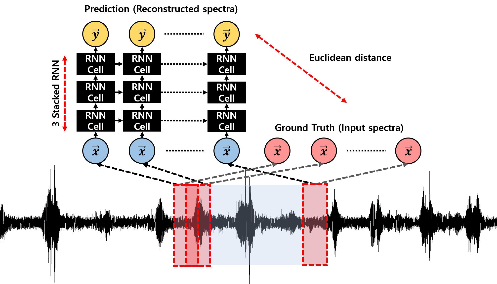
First, we sliced the entire sound data in 500 ms with overlapping. It helps learning the data easily for the model because it provides redundant information between each sequence. After slicing, we applied STFT and MFCC feature extraction respectively to each slice. We used the Hann window for windowing, 2048 for window length, and 512 for hop length in STFT. Each spectra consists of spectrum to spectrum after STFT or MFCC feature extraction. The symbol k means the number of window used in preprocessing. Finally, we calculated a time-averaged spectrum using Equation (1) and normalized the range of magnitude from 0 to 1. The procedure of obtaining time-averaged spectrum is shown in Figure 1 and sample of preprocessed data is shown in Figure 2:
The spectrum of spectra obtained after preprocessing can be used directly. However, we used a time-averaged spectrum because it could ease minute noise generated during machine operation. Therefore, we used a time-averaged spectrum to construct input and ground truth for FARED. We refer to the spectrum for construct input data as and output spectrum of FARED as . Dimensions of the and were the same as 192 k, 1025 and 128 for raw data, spectrum from STFT and MFCC feature extraction, respectively. We used data preprocessed by STFT and MFCC feature extraction for experiments.
3. Fast Adaptive RNN Encoder–Decoder
In this section, we will present the architecture of FARED based on RNN Encoder–Decoder. We used Long-Short Term Memory (LSTM) for each RNN cell. We will also describe the training algorithm and how to calculate the number of parameters of FARED.
3.1. RNN Encoder–Decoder Based Architecture
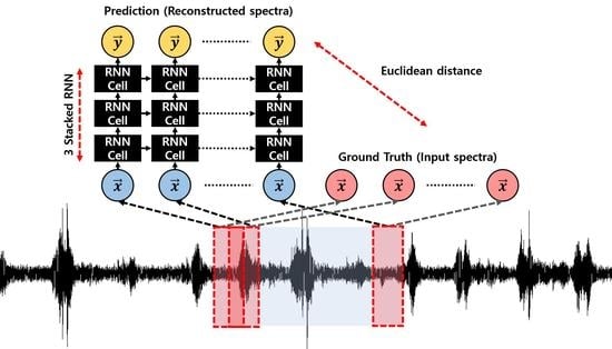
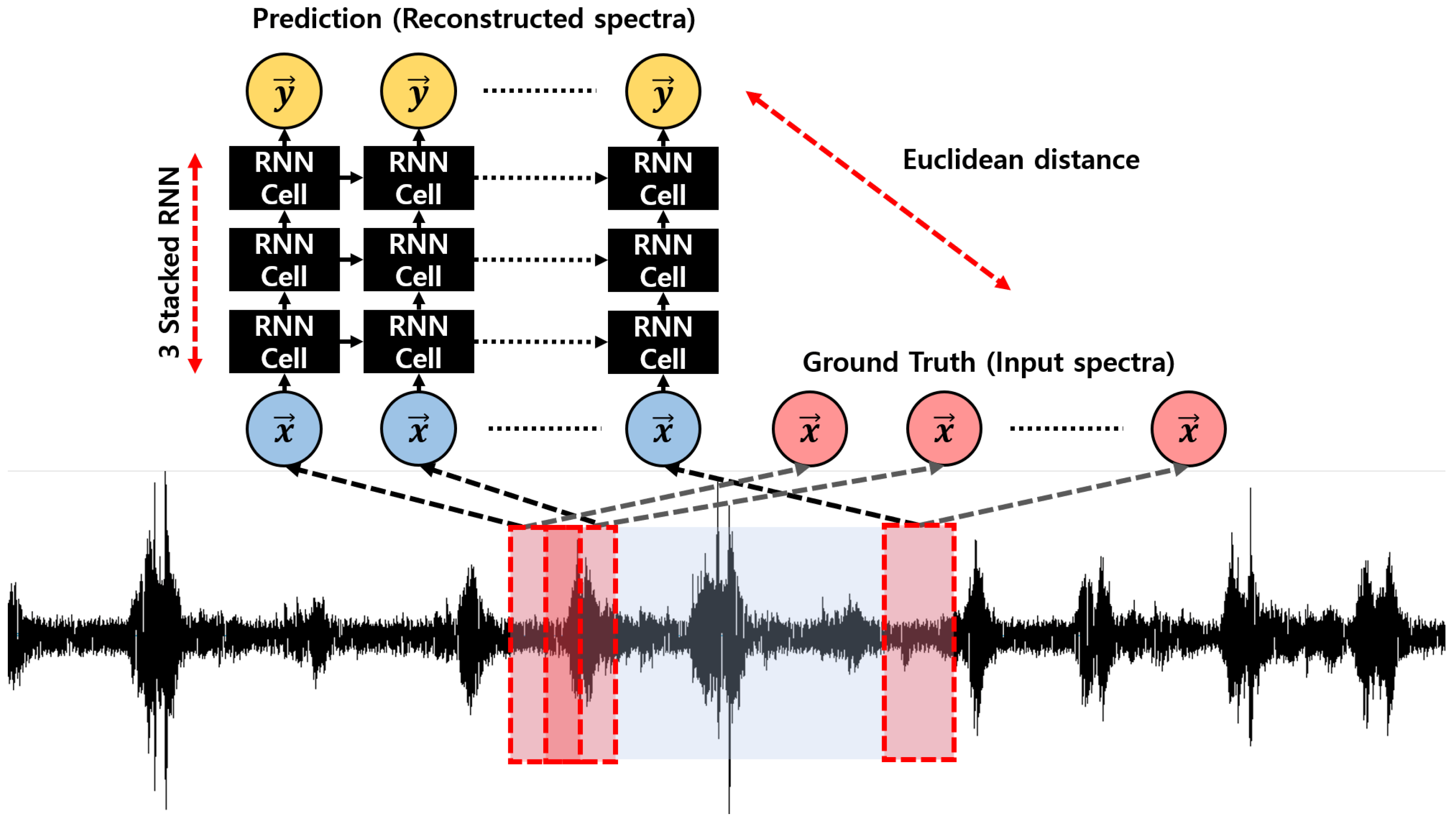
RNN Encoder–Decoder is one of the generative models generally used for machinet translation [1,2]. FARED is designed for reconstructing input sequences as shown in Figure 3. The learning method in the form of conditional probability and generative model already given for FARED is shown as follows:
In Equation (2), and are a set of sequential input and output spectrum ( and ), respectively. The is the posterior score (uncertainty), is likelihood, and is prior knowledge. We have information of prior knowledge and posterior score from the training data. Therefore, the information that we want to know is likelihood. It will be learned by the maximum likelihood estimation in the training process.
FARED based on RNN Encoder–Decoder is presented in Figure 3. Some research studies have used the model for predicting future sequence from current sequence [13,14]. We refer to the model used in a previous research, ‘Ref-RED’. FARED is a modified model of Ref-RED. When Ref-RED is used to predict repeated future sequence, it works well. For example, Ref-RED works well to anomaly detection in Electrocardiography (ECG) because the pattern of ECG has one-to-one correspondence. For example, only R wave appears after Q wave in normal ECG. The SMD assembly machine has one-to-many correspondence that makes it difficult to learn and predict future sequence. Therefore, we modified Ref-RED to FARED to restore the current sequence like conventional AE [8,9] because it is easy to learn by restoring the current sequence rather than predicting future sequence. We need a fast adaptation model for the manufacturing environment. Thus, we need to find a model that learns data easier and faster. We have performed experiments to compare multiple REDs for finding the better model [15]. In that experiment, we confirmed that a structure like FARED could learn the data more effectively than others.
To detect anomalies in real time, it is necessary to decide if the input is abnormal or not in a short period. FARED also has shorter decision time than Ref-RED. Assuming that the length of the input and output sequence are equal to L, Ref-RED decides anomaly or not in times because it needs to observe the input sequence and the next L sequences for decision. However, FARED needs only L time for decision. This means that FARED is a more efficient model. FARED, the model that we proposed, can be called, ‘Fast Adaptive’. We will show that FARED is ‘Fast Adaptive’ through experiments in Section 4.3.
We trained FARED to learn the likelihood with only normal state data, so it can generate input sequences well when input sequences were normal state sequences. However, if the sequence of the input data was shuffled or not observed in the training data, FARED could not function well due to the low likelihood that the model knew. The training algorithm is presented in Algorithm 1. The input data consists of p sequential spectrum while the output data also has the same length of sequential spectrum. Sequential vectors are obtained after preprocessing as shown in Section 2. We initialized parameters of the neural network using Xavier initializer [16]. The purpose of Algorithm 1 is to minimize the Euclidean distance between and . We used RMSprop optimizer for minimizing [17].
| Algorithm 1 Training algorithm for RNN Encoder–Decoder |
| Input: Set of the sequential input spectrum |
| Output: Set of the sequential output spectrum |
| Initialize network parameters by Xavier initializer |
| while the loss has not converged do |
| Compute loss between and using Euclidean distance [16] |
| Update parameters by RMSprop optimizer [17] |
| end while |
3.2. Long-Short Term Memory
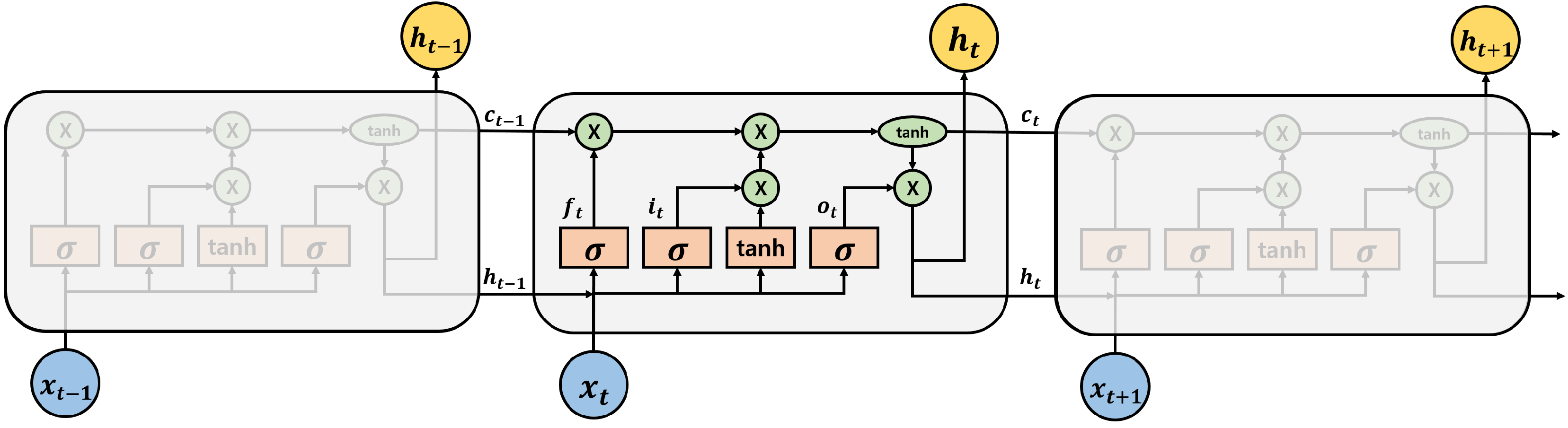
In the RNN Encoder–Decoder, the RNN cell can be selectively used in vanilla RNN [18], Long- Short Term Memory (LSTM) [19], and Gated Recurrent Unit (GRU) [20]. We used LSTM for constructing the model. This is because vanilla RNN has vanishing gradient problem when the length of input or output sequences becomes long. We can also consider using GRU. However, Chung et al. [21] have already reported that there is no superiority between LSTM and GRU. Therefore, we used LSTM for constructing FARED. Each LSTM cell has three types of gates and two types of states as follows:
Equations (3) to (5) present three types of gates. Two types of states are shown in Equations (6) and (7). For each equation, is the input vector (spectrum), is cell state vector, and is the hidden state vector of the LSTM. is the same as the output spectrum , and each W, U, b of equations are the parameter of the LSTM. Forget gate, input gate and output gate’s activated vectors are , , respectively. The ∘ symbol in Equations (6) and (7) means Hadamard products. Figure 4 shows the structure of the LSTM and it contains all of the equations. Equations and Figure 4 show that LSTM derives output with causality. RNN derives output using the same parameter for every divided input. Thus, RNN can process the same size of data with a smaller number of parameters than AE.
We can calculate the number of parameters P of the proposed model with dimension of the cell state (), input () and output () as follows [22]:
The proposed model is constructed by three stacked LSTM and its input dimension is 128 when using the MFCC feature extraction shown in Figure 2. Table 2 shows the number of parameters P of two models. AE by Oh and Yun [10] has about 11 times as many parameters than FARED that means AE requires more time to train the parameters than FARED and more computational resources.
4. Experiments
In this section, we will explain how we acquire the dataset. We also compared and confirmed the performance of FARED in anomaly detection as well as fast adaptation with previous works.
4.1. Dataset
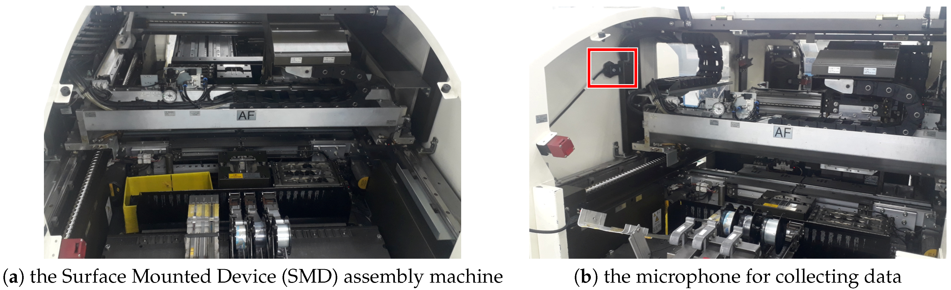
The dataset (CREVIS Co., Ltd.,Yongin, Korea) consisted of sound data acquired from SMD assembly machine with 192 kHz of sampling rate. The data collection process is shown in Figure 5. Sequential machine operational sound data were collected from an operating SMD assembly machine placing a microphone as indicated by the red bounding box in Figure 5b.
The collected dataset is summarized in Table 3. Sample data and source code are available at the Github repository [23]. We experimented with one of the data collected from each manufacturing process as normal while the others were abnormal. This meant that all manufacturing processes were made abnormal except for itself.
We used another dataset from previous research of Oh and Yun [10] to confirm that FARED could detect anomalies well as shown in Table 4. One cycle in each class in Table 4 is equal to 20 s because it belongs to the same manufacturing process. We refer to the dataset in Table 3 as ‘Set-A’ and that in Table 4 as ‘Set-B’.
The whole data of Set-B were collected from the same SMD production. Abnormal state data were ‘Intermittent noise’ and ‘Non-greased’. The ‘Intermittent noise’ class contained ‘Air ejection’, an action to remove the foreign substance in the machine, and ‘Artifact’, a clacking sound made by human. The ‘Non-greased’ class was collected when the machine operated without grease.
4.2. Comparison of Preprocessing Methods
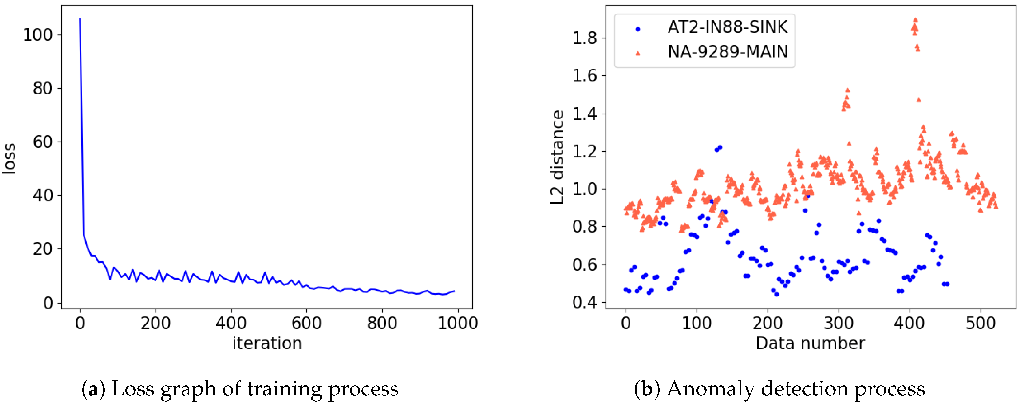
In this section, we compared two types of data preprocessing technique with Set-A in order to construct faster adaptive architecture. We trained FARED with STFT and MFCC feature extraction respectively and compared them to determine which preprocessing technique was more appropriate for FARED. Sequences from only one SMD product were regarded as normal while others were considered as abnormal. We used normal state data for training. Results of training FARED are presented in Figure 6. Seven cycles for each class were performed separately for training. The rest of testing was then performed. The input data with a set of 30 sequences was constructed. The output had the same shape as the input. One sequence contained 500 ms information of sound data and overlapping was applied when slicing the whole sound data. Thus, 30 sequences hold 8 s of information. When using the data preprocessed by STFT, it took about 25 min for training. However, MFCC took only about 3 min because of data dimension. Compared to AE based model proposed by Oh and Yun [10] that took 8 h for training with a set of 32 sequences, 25 min were relatively short. Given preparation time in Table 1, STFT is not appropriate for preprocessing. We also found that 192k-dimensional raw data larger than STFT were not appropriate for usage. MFCC can be preferably trained and used in near real time because of the smaller dimension of the data and reduced a number of parameters.
We measured the Area Under the Curve (AUC) from the Receiver Operating Characteristic (ROC) curve as an indicator of performance [24]. We constructed the ROC curve with lowest to highest reconstruction error as thresholds. In addition, it is possible to find the adequate threshold for filtering out anomalies for each normal state in ROC curve. Results of AUC are shown in Table 5. The AUC is closer to 1 when the model filters out anomalies effectively. It is closer to 0 otherwise.
The performance of FARED when using MFCC is lower than that when using STFT. However, MFCC has an advantage such as reduction of training time for about one-tenth than using STFT because of decreased data dimension from 1025 to 128. This was why MFCC feature extraction was used in our model for fast adaptation. If sufficient preparation time is given, we may consider using STFT.
4.3. Fast Adaptive Architecture
The fast-adaptive architecture is shown in Section 3.1. In this section, we confirmed that FARED could adapt faster than Ref-RED with Set-B. We show how faster FARED can adapt to various environments for anomaly detection than previous RNN Encoder–Decoder architecture. We will also compare the anomaly detection performance and the number of parameters with AE used by Oh and Yun [10]. We separated seven cycles of each class for training and the rest for testing. We trained ‘Normal’ class and tested others for detecting anomalies. Results of anomaly detection are shown in Figure 7 and Table 6.
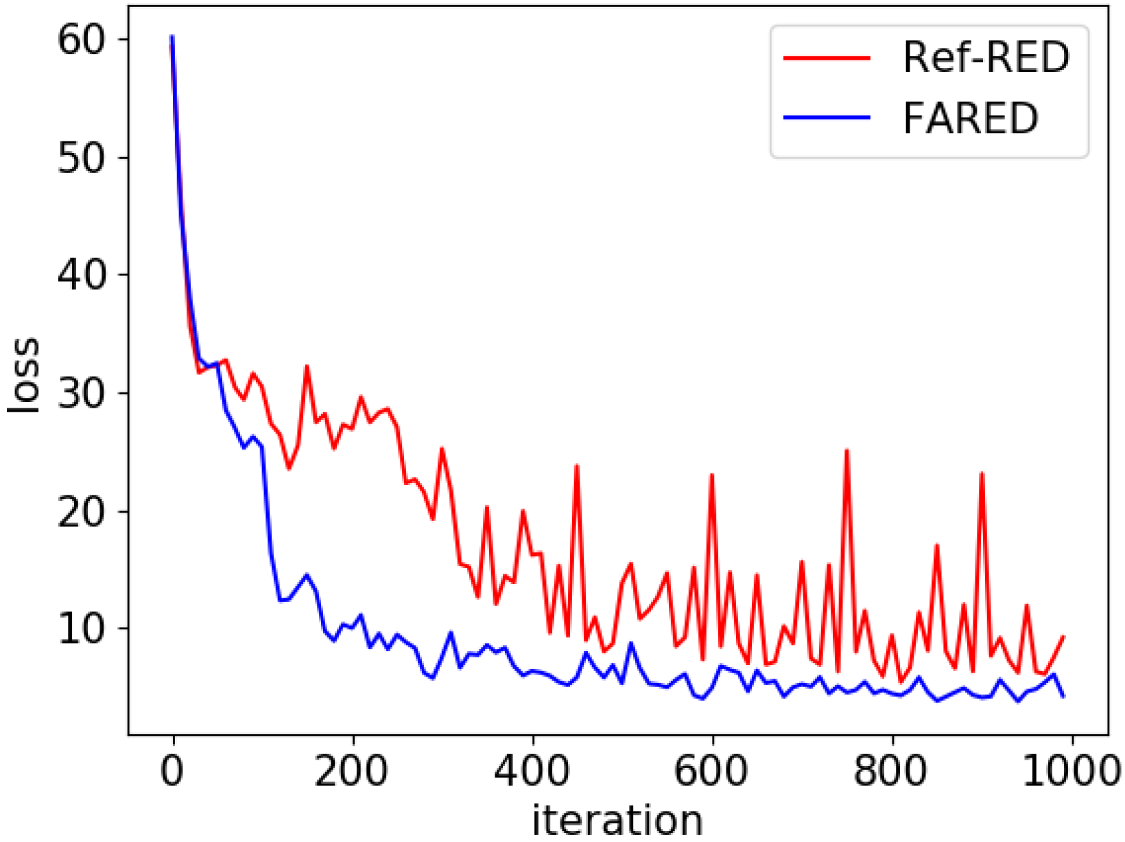
Figure 7 shows that the loss of FARED converges faster than Ref-RED. Since fast adaptation is the most important issue in this research, FARED is more appropriate than Ref-RED. Moreover, the scale of oscillation is significantly reduced because FARED has more stability and reliability.
The average AUC of FARED is the best among three generative models as shown in Table 6. We experimented Ref-RED and FARED in the same conditions such as learning rate, training iterations, and the number of parameters as those used in a previous work [15]. However, FARED is 0.118 (16%) higher than the average AUC of Ref-RED for anomaly detection. This means that FARED adapts faster for detecting anomalies than Ref-RED in the manufacturing environment. That was the reason why we called the architecture ‘Fast Adaptive’.
Furthermore, we achieved higher performance on anomaly detection by using FARED than AE based architecture. Oh and Yun have achieved AUC of 0.980 at ‘Intermittent noise’ and 0.640 at ‘Non-greased’. FARED had lower AUC at ‘Intermittent noise’ than AE, but much better at ‘Non-greased’. The reason for detecting ‘Non-greased’ much better than ‘Intermittent noise’ using FARED is that ‘Non-greased’ set has persistent abnormality while ‘Intermittent noise’ does not have persistent abnormality. ‘Intermittent noise’ has almost the same features as normal operation except for a specific abnormal section.
5. Conclusions
In the actual field, the manufacturing process is very flexible because of small quantity batch production. Therefore, in varied environments like ours, it is practically difficult to use the previous anomaly detection model based on AE because they require huge storage resources and long training time.
However, our model, FARED, has the ability of fast adaptation that AE or Ref-RED does not have. FARED can adapt in three minutes for the new manufacturing process. It only needs small computational resources. The reason why training time and computational resource were reduced was due to the structure of FARED and data preprocessing.
In the future, we need to find a compromise preprocessing technique between STFT and MFCC feature extraction for better performance of anomaly detection. To make our model more useful, we also need to classify anomalies. Currently, our model FATED is an unsupervised learning model that cannot define the kind of anomaly is. An ensemble with a classification model that can limitedly classify abnormal states might be needed.
Author Contributions
All authors contributed to manuscript preparation of the paper. Il Dong Yun collected sound data of SMD machine operation and designed the experiments. YeongHyeon Park implemented the overall schematic of the proposed method for anomaly detection with fast adaptation, and wrote the manuscript. All authors reviewed and approved the final manuscript.
Funding
This research was supported by grant (2017R1A2B4004503) of the Basic Science Research Program through the National Research Foundation (NRF) funded by the Ministry of Education, Science, and Technology, Republic of Korea. It was also supported by Hankuk University of Foreign Studies Research Fund of 2018.
Conflicts of Interest
The authors declare no conflict of interest.
References
- Cho, K.; Van Merriënboer, B.; Gulcehre, C.; Bahdanau, D.; Bougares, F.; Schwenk, H.; Bengio, Y. Learning phrase representations using RNN encoder-decoder for statistical machine translation. arXiv, 2014; arXiv:1406.1078. [Google Scholar]
- Sutskever, I.; Vinyals, O.; Le, Q.V. Sequence to sequence learning with neural networks. In Advances in Neural Information Processing Systems 27; NIPS: Montreal, QC, Canada, 2014; pp. 3104–3112. [Google Scholar]
- Lee, J.; Choi, H.; Park, D.; Chung, Y.; Kim, H.Y.; Yoon, S. Fault detection and diagnosis of railway point machines by sound analysis. Sensors 2016, 16, 549. [Google Scholar] [CrossRef] [PubMed]
- Abdi, M.J.; Giveki, D. Automatic detection of erythemato-squamous diseases using PSO–SVM based on association rules. Eng. Appl. Artif. Intell. 2013, 26, 603–608. [Google Scholar] [CrossRef]
- Potes, C.; Parvaneh, S.; Rahman, A.; Conroy, B. Ensemble of feature-based and deep learning-based classifiers for detection of abnormal heart sounds. In Proceedings of the Computing in Cardiology Conference (CinC 2016), Vancouver, BC, Canada, 11–14 September 2016; pp. 621–624. [Google Scholar]
- Cortes, C.; Vapnik, V. Support-vector networks. Mach. Learn. 1995, 20, 273–297. [Google Scholar] [CrossRef] [Green Version]
- Krizhevsky, A.; Sutskever, I.; Hinton, G.E. Imagenet classification with deep convolutional neural networks. In Proceedings of the Twenty-sixth Conference on Neural Information Processing Systems, Lake Tahoe, NV, USA, 3–8 December 2012; pp. 1097–1105. [Google Scholar]
- Deng, L.; Seltzer, M.L.; Yu, D.; Acero, A.; Mohamed, A.R.; Hinton, G. Binary coding of speech spectrograms using a deep auto-encoder. In Proceedings of the Eleventh Annual Conference of the International Speech Communication Association, Chiba, Japan, 26–30 September 2010. [Google Scholar]
- Mao, X.; Shen, C.; Yang, Y.B. Image restoration using very deep convolutional encoder-decoder networks with symmetric skip connections. In Proceedings of the Thirtieth Conference on Neural Information Processing Systems, Barcelona, Spain, 5–10 December 2016; pp. 2802–2810. [Google Scholar]
- Oh, D.; Yun, I. Residual Error Based Anomaly Detection Using Auto-Encoder in SMD Machine Sound. Sensors 2018, 18, 1308. [Google Scholar] [CrossRef] [PubMed]
- Muda, L.; Begam, M.; Elamvazuthi, I. Voice recognition algorithms using mel frequency cepstral coefficient (MFCC) and dynamic time warping (DTW) techniques. arXiv, 2010; arXiv:1003.4083. [Google Scholar]
- Han, W.; Chan, C.F.; Choy, C.S.; Pun, K.P. An efficient MFCC extraction method in speech recognition. In Proceedings of the ISCAS 2006 IEEE International Symposium on Circuits and Systems, Island of Kos, Greece, 21–24 May 2006; p. 4. [Google Scholar]
- Chauhan, S.; Vig, L. Anomaly detection in ECG time signals via deep long short-term memory networks. In Proceedings of the 2015 IEEE International Conference on Data Science and Advanced Analytics (DSAA), Paris, France, 19–21 October 2015; pp. 1–7. [Google Scholar]
- Malhotra, P.; Vig, L.; Shroff, G.; Agarwal, P. Long short term memory networks for anomaly detection in time series. In Proceedings of the 2015 European Symposium on Artificial Neural Networks, Computational Intelligence and Machine Learning, Bruges, Belgium, 22–24 April 2015; p. 89. [Google Scholar]
- Park, Y.; Yun, I.D. Comparison of RNN Encoder–Decoder Models for Anomaly Detection. arXiv, 2018; arXiv:1807.06576. [Google Scholar]
- Glorot, X.; Bengio, Y. Understanding the difficulty of training deep feedforward neural networks. In Proceedings of the Thirteenth International Conference on Artificial Intelligence and Statistics, Sardinia, Italy, 13–15 May 2010; pp. 249–256. [Google Scholar]
- Kingma, D.P.; Ba, J. Adam: A method for stochastic optimization. arXiv, 2014; arXiv:1412.6980. [Google Scholar]
- Mikolov, T.; Karafiát, M.; Burget, L.; Černockỳ, J.; Khudanpur, S. Recurrent neural network based language model. In Proceedings of the Eleventh Annual Conference of the International Speech Communication Association, Chiba, Japan, 26–30 September 2010. [Google Scholar]
- Hochreiter, S.; Schmidhuber, J. Long short-term memory. Neural Comput. 1997, 9, 1735–1780. [Google Scholar] [CrossRef] [PubMed]
- Chung, J.; Gulcehre, C.; Cho, K.; Bengio, Y. Gated Feedback Recurrent Neural Networks. arXiv, 2015; arXiv:1502.02367. [Google Scholar]
- Chung, J.; Gulcehre, C.; Cho, K.; Bengio, Y. Empirical evaluation of gated recurrent neural networks on sequence modeling. arXiv, 2014; arXiv:1412.3555. [Google Scholar]
- Sak, H.; Senior, A.; Beaufays, F. Long short-term memory recurrent neural network architectures for large scale acoustic modeling. In Proceedings of the Fifteenth Annual Conference of the International Speech Communication Association, Singapore, 14–18 September 2014. [Google Scholar]
- Github. Available online: https://github.com/YeongHyeon/FARED_for_Anomaly_Detection (accessed on 4 September 2018).
- Fawcett, T. An introduction to ROC analysis. Pattern Recognit. Lett. 2006, 27, 861–874. [Google Scholar] [CrossRef]
Figure 1.
The process for obtaining the average spectrum of spectra. (a) original spectra obtained from Short-Time Fourier Transform (STFT) or Mel-Frequency Cepstral Coefficients (MFCC) feature extraction; (b) sliced by time axis spectra according to the number of window used in STFT or MFCC feature extraction; (c) average of sliced spectra.

Figure 2.
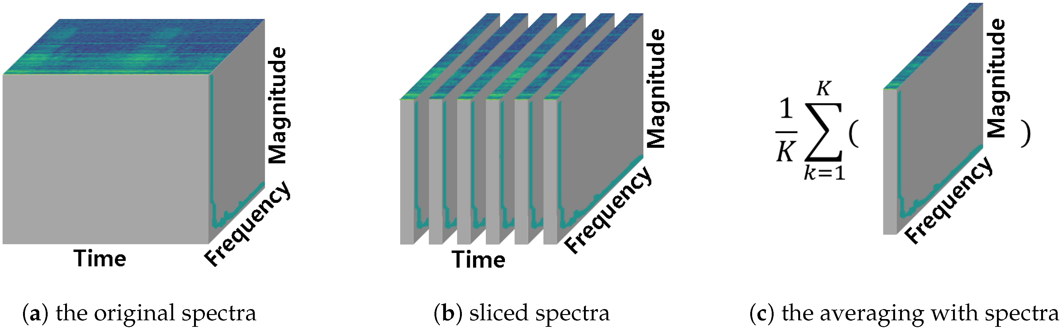
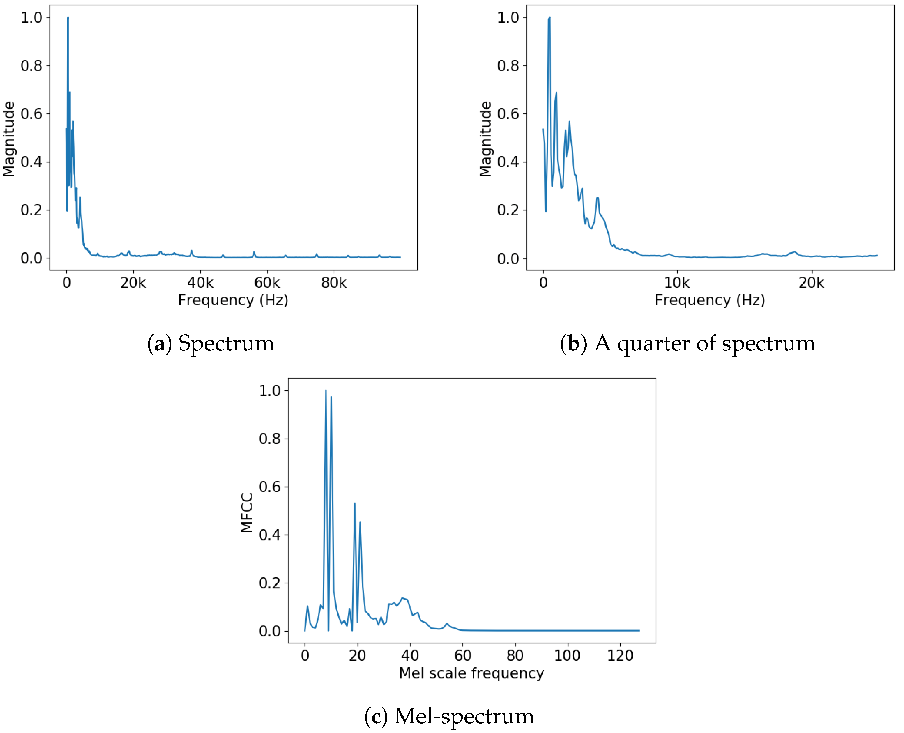
Subfigures (a,b) are time-averaged spectrum after STFT and (c) is 128-dimensional time-averaged Mel-spectrum after MFCC feature extraction. (a) represents a range of 96 kHz, with a resolution of 1025; (b) is an expanded view of a quarter of (a). Each unit of (c) represents one MFCC filter bank.
Figure 2.
Subfigures (a,b) are time-averaged spectrum after STFT and (c) is 128-dimensional time-averaged Mel-spectrum after MFCC feature extraction. (a) represents a range of 96 kHz, with a resolution of 1025; (b) is an expanded view of a quarter of (a). Each unit of (c) represents one MFCC filter bank.

Figure 3.
Structure of Fast Adaptive Recurrent Neural Network (RNN) Encoder–Decoder (FARED). The input is constructed by sequential spectrum (red box). Each spectrum has of overlapping in the time domain. The output is a sequential reconstructed spectrum from input sequences. The Euclidean distance between prediction and ground truth is used for training and anomaly detection.

Figure 4.
The structure of the Long-Short Term Memory (LSTM) cell. It contains input gate , output gate, , forget gate , hidden state and cell state . The symbol means sigmoid function and tanh means hyperbolic tangent function.
Figure 4.
The structure of the Long-Short Term Memory (LSTM) cell. It contains input gate , output gate, , forget gate , hidden state and cell state . The symbol means sigmoid function and tanh means hyperbolic tangent function.

Figure 5.
The SMD assembly machine with microphone. The microphone that is attached as shown in (b) is used for collecting sound data when the machine is operating.
Figure 5.
The SMD assembly machine with microphone. The microphone that is attached as shown in (b) is used for collecting sound data when the machine is operating.

Figure 6.
Results of the training and detection process. When GTX 1060 3 GB for 1 k iteration with minibatch size 100 was used, it took about three minutes when using MFCC. The ’NA-9289-MAIN’ is regarded as abnormal while ‘AT2-IN88-SINK’ is regarded as normal. FARED can distinguish between ‘AT2-IN88-SINK’ and ‘NA-9289-MAIN’ as shown in subplot (b).

Figure 7.
Comparison of Ref-RED and FARED training process. It shows that loss of the FARED converges faster and more stable than Ref-RED under same conditions (1 k iterations with minibatch size 100 of training and 0.005 of learning rate).
Figure 7.
Comparison of Ref-RED and FARED training process. It shows that loss of the FARED converges faster and more stable than Ref-RED under same conditions (1 k iterations with minibatch size 100 of training and 0.005 of learning rate).


Table 1.
Daily record of the manufacturing process on 24 April 2018.
| Product Name | Production Amount | Preparing Time (min:s) | Cycle Time (s) | Running Time (min) |
|---|---|---|---|---|
| CT-C134-BOT | 50 | - | 27 | 25 |
| CT-C134-TOP | 50 | 4:27 | 30 | 37 |
| ST-3118 | 30 | 10:41 | 17 | 36 |
| ST-4214-GE | 20 | 9:24 | 12 | 28 |
| NA-9473 | 60 | 8:40 | 13 | 57 |
| M-3808 | 8 | 30:11 | 15 | 20 |
| M-3708 | 8 | 10:09 | 13 | 45 |
| M-4178 | 8 | 15:40 | 24 | 24 |
| M-4478 | 8 | 6:07 | 18 | 23 |
| Average | 26 | 10:35 | 18 | 32 |
Table 2.
Comparison of the number of the parameters.
| Model | Auto-Encoder [10] | Fast Adaptive RNN Encoder–Decoder (FARED) |
|---|---|---|
| Number of parameters | 4,864,160 | 443,520 |
Table 3.
Dataset collected from Surface Mounted Device (SMD) assembly machine (Set-A).
| Product Name | Number of Cycle | Cycle Time (s) | Total Time (s) |
|---|---|---|---|
| AT2-IN88-SINK | 63 | 8 | 527 |
| M-3708 | 8 | 13 | 121 |
| M-4478 | 8 | 18 | 165 |
| NA-9289-MAIN | 55 | 10 | 581 |
| NA-9473 | 53 | 13 | 696 |
| ST-4214-GE | 9 | 12 | 114 |
Table 4.
Dataset collected from same manufacturing process (Set-B) [10].
Table 4.
Dataset collected from same manufacturing process (Set-B) [10].
| Class | Number of Cycle | Cycle Time (s) | Total Time (s) |
|---|---|---|---|
| Intermittent noise | 41 | 20 | 836 |
| Non-greased | 8 | 20 | 164 |
| Normal | 23 | 20 | 470 |
Table 5.
Area Under the Curve (AUC) matrix of anomaly detection using Mel-Frequency Cepstral Coefficients (MFCC) feature extraction.
Table 5.
Area Under the Curve (AUC) matrix of anomaly detection using Mel-Frequency Cepstral Coefficients (MFCC) feature extraction.
| Normal | Short-Time Fourier Transform (STFT) | Mel-Frequency Cepstral Coefficients (MFCC) |
|---|---|---|
| AT2-IN88-SINK | 0.996 | 1.000 |
| M-3708 | 0.992 | 0.865 |
| M-4478 | 0.999 | 0.999 |
| NA-9289-MAIN | 0.890 | 0.712 |
| NA-9473 | 0.965 | 0.806 |
| ST-4214-GE | 0.978 | 0.983 |
| Average | 0.970 | 0.894 |
Table 6.
AUC of anomaly detection in the same manufacturing process.
| Model | Intermittent Noise | Non-Greased | Average |
|---|---|---|---|
| Ref-RED | 0.835 | 0.634 | 0.735 |
| Auto-Encoder | 0.980 | 0.640 | 0.810 |
| FARED | 0.724 | 0.983 | 0.853 |
© 2018 by the authors. Licensee MDPI, Basel, Switzerland. This article is an open access article distributed under the terms and conditions of the Creative Commons Attribution (CC BY) license (http://creativecommons.org/licenses/by/4.0/).
Share and Cite
MDPI and ACS Style
Park, Y.; Yun, I.D. Fast Adaptive RNN Encoder–Decoder for Anomaly Detection in SMD Assembly Machine. Sensors 2018, 18, 3573. https://0-doi-org.brum.beds.ac.uk/10.3390/s18103573
AMA Style
Park Y, Yun ID. Fast Adaptive RNN Encoder–Decoder for Anomaly Detection in SMD Assembly Machine. Sensors. 2018; 18(10):3573. https://0-doi-org.brum.beds.ac.uk/10.3390/s18103573
Chicago/Turabian StylePark, YeongHyeon, and Il Dong Yun. 2018. "Fast Adaptive RNN Encoder–Decoder for Anomaly Detection in SMD Assembly Machine" Sensors 18, no. 10: 3573. https://0-doi-org.brum.beds.ac.uk/10.3390/s18103573
Note that from the first issue of 2016, this journal uses article numbers instead of page numbers. See further details here.