1. Introduction
Since seminal work by from Morris [
1], MEMS accelerometers and gyroscopes have been increasingly used for the real-time measurement of body motion spatio-temporal parameters, due to their low consumption and cost, and their easy connectivity. Specifically, they are the base component for wearable devices that measure linear and/or angular displacements in the human body, e.g., the shank rotation, the stride length, and the pelvis displacement. The stride length is needed, for example, in pedestrian navigation systems [
2] or for clinical gait analysis [
3]. The pelvis displacement is useful in rehabilitation or prosthetics, as an indicator of the metabolic cost in walking [
4], to discriminate left and right steps [
5], or to estimate the step length [
6,
7,
8].
Although particularly convenient for real-time applications, these MEMS-based estimations suffer the problem of an unbounded error growth with time [
9]. For angular displacements, the problem is usually addressed by the sensor integration of gyroscopes, accelerometers, and magnetic field sensors, by means of Kalman-filtering-like algorithms, forming inertial measurement units (IMU) [
10].
However, for linear displacements, there is no unique accepted solution. The basic principle of accelerometers as linear position sensors is straightforward: the measured acceleration is converted to a linear position by doubly integrating the accelerometer data, that is, by adding up a noisy signal coming from a sensor supposedly aligned in a measurement axis. However, error grows too fast with time, making it mandatory to provide some kind of error compensation. Otherwise, the results can be unacceptable for most applications, even if integration is made in short time slots.
The main error source comes from sensor bias and the duration of the integration time. Bias is the difference between the sensor output and the true value and it has multiple origins, both deterministic and stochastic. Deterministic bias sources are those that could be predicted, and possibly corrected by a per device calibration. On the contrary, stochastic bias sources can be considered random and need to be compensated. They are probabilistically modeled, in the form of power spectral density or Allan variance, and they have a variety of origins: velocity random walk (additive white noise), bias instability (flicker noise), quantization noise, sinusoidal errors, rate random walk, and rate ramp [
11]. A possible general model of the accelerometry measurement process could be
being the sensor output,
the real acceleration to be measured,
S the scale factor,
a temperature-dependent bias,
a time-dependent non-linear bias function, and
the bias error caused by stochastic sources [
12]. If a certain bias in acceleration is integrated, it will produce an error in distance estimation which grows quadratically with the integration time [
13]. Then, integration time is a key parameter to consider when studying distance estimation errors.
In spite of the widespread use of this measurement technique in real-time human-motion-related applications, there is a lack of agreement about how to define and compensate its errors. The error-correction methods proposed in the literature are heuristic in nature and do not provide a general design criteria. It is not clear how different error sources behave with integration time [
9] or how to evaluate the relative weight of each source in the final results.
In this paper, we aim to shed try to put some light on this problem by making a systematic comparison of different distance estimation methods with different sensors, to check if they are compatible with the demands imposed by ambulatory human motion monitoring applications: accuracy in real-time and robustness to various experimental kinematic conditions.
The presented results confirm that it is possible to use accelerometers to estimate short linear displacements of the body with a 4.5% error in typical conditions. However, it is also shown that the motion conditions, such as mean velocity and acceleration profiles, can be a key factor in the performance of this estimation, as the dynamic response of the accelerometer can affect the results. The study sets out the basis for a systematic design of distance estimations, and it provides a tool to better interpret their results depending on the experimental conditions.
Section 2 will develop the distance estimation problem and its experimental conditions in the context of human motion science.
Section 3 will detail the estimation methods selected and the design and conditions of the experiments. The results will be explained in
Section 4 and discussed in
Section 5. The main conclusions will be synthesized in
Section 6.
2. Real-Time Distance Estimation for Cyclic Motion
In human movement science (HMS), most distance estimations of interest are not the result of a free linear motion, but rather they are related to cyclical or periodical motions, such as human walking. For example, the body center of mass moves up (vCOM) and sideways (mlCOM) to its maximum twice each stride in normal gait or the distance traveled by one foot between two consecutive heel strike events, which defines the stride length (SL).
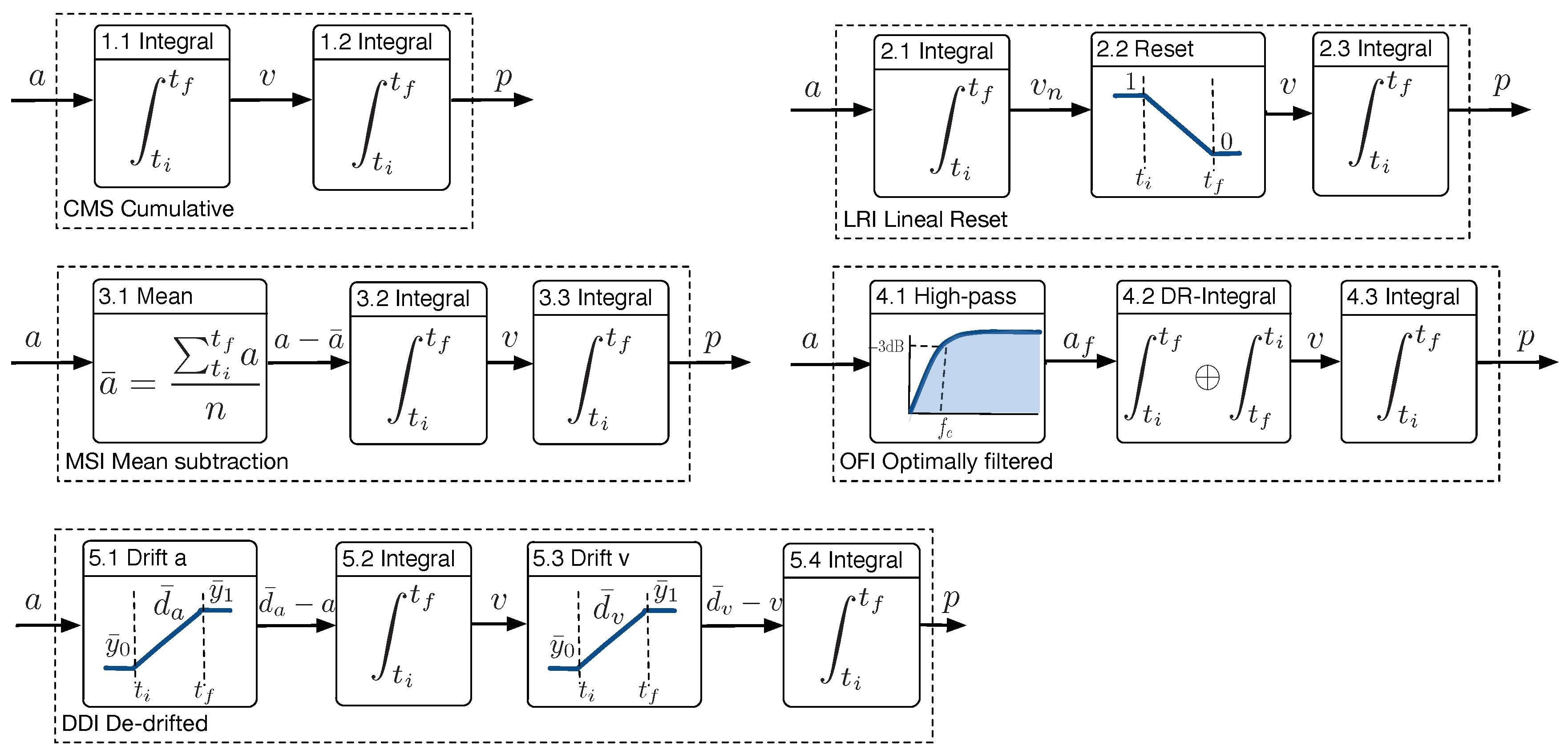
Several distance estimation methods have been proposed in the human movement science literature. In spite of its known limitations, the simple direct cumulative double integration (CMS) method has been applied to estimate the stride length in devices for the ambulatory analysis of gait [
14]. We will test this method as a worst-case scenario for distance estimation. Other methods, see
Figure 1, try to mitigate the growth of error caused by the direct signal integration, because they are noticeable even within the short time integration periods of interest (0.4–1.6 s).
In Ref. [
15], the direct method is slightly modified for both horizontal and vertical motion of the foot, to estimate the step length. Previous to the second integral, a lineal resetting mechanism is applied to the velocity by weighting linearly between 1 and 0 during the integration time (LRI method). This is to ensure that
, a biomechanics property that both foot velocities were supposed to have. The authors claim that the aim of the method is to remove measurement error due to noise and drift.
An integration with mean subtraction (MSI method) is proposed in Ref. [
8] to estimate zCOM displacements from COM accelerations, and in Ref. [
16] for foot displacements, both in the context of gait analysis. The idea was to remove the non-zero medium value
caused by sensor artifacts and uncertainties, prior to the first velocity integration. The mean value of the acceleration between two consecutive integration events (ipso-lateral heel strikes)
was subtracted, and a first integration was made to estimate the instantaneous velocity. Notice that forcing the acceleration to have a zero mean value is equivalent to assuming that the velocity is the same at the beginning and the end of the segment, for example, if the motion comes to rest at the end of the period,
being the average acceleration in the segment period, and
. In Ref. [
8], the mean subtraction was applied twice in the particular case where the final position is the same at the beginning and end of the integration period, but this case will not be addressed here.
In Ref. [
17], a technique is presented to estimate the stride length by integration of the body antero-posterior (forward) acceleration, measured at the pelvis. It is denominated as the optimally filtered integration (OFI method). To reduce the low frequency acceleration noise, at each gait cycle, the acceleration signal was high-pass-filtered, with a 2nd order Butterworth filter with an
Hz cut frequency, calculated from data of a given gait cycle with known equal initial and final velocities. After filtering, a first integration produced instantaneous velocity. Taken from Ref. [
18], the numerical method chosen to integrate the data was the Cavalieri–Simpson. If the so-estimated final velocity is close to the initial velocity, they are supposed as equal, and a weighted direct and reverse integration is applied, aimed to reduce the time drift in velocity. Notice that this method, contrary to the LRI and MSI methods, did not need a general assumption about the velocity at the end of the integration time, because the authors were dealing with a biomechanics problem (apCOM) with different characteristics.
A different method is proposed in Ref. [
19], named de-drifted integration (DDI method). It encompasses the subtraction of a weighted mean function of data samples, previous to each of both integrations. In this case, it was applied to instep foot accelerations during a stride time cycle, with no previous filters, to estimate the stride length. The acceleration drift function was computed by averaging a few initial and final accelerometry samples and by removing a lineal interpolation between both values from the original signal. The size of both sets of samples was empirically selected. The velocity drift function was based on the assumption of zero velocity at the beginning and end of the step, and a lineal function from zero to the mean of the last velocity samples was subtracted from to achieve it.
Other methods have been proposed in human motion analysis for distance estimation that will not be included in this study. In Ref. [
3], zCOM and mlCOM displacements are estimated in two steps: (1) filtering the sensor data before the double integration with a low-pass 4th order zero-lag Butterworth filter, at a 20 Hz cut frequency, to remove acceleration noise and (2) filtering the distance estimation after the double integration with a high-pass 4th order zero-lag Butterworth filter, at a 0.1 Hz cut frequency, to remove its long-term time drift. This drift filtering has to be made in longer time intervals (30 s in Ref. [
3] or 12–18 s in Ref. [
7]). These are useful solutions for off-line data analysis, but not feasible for real-time step-to-step applications.
3. Materials and Methods
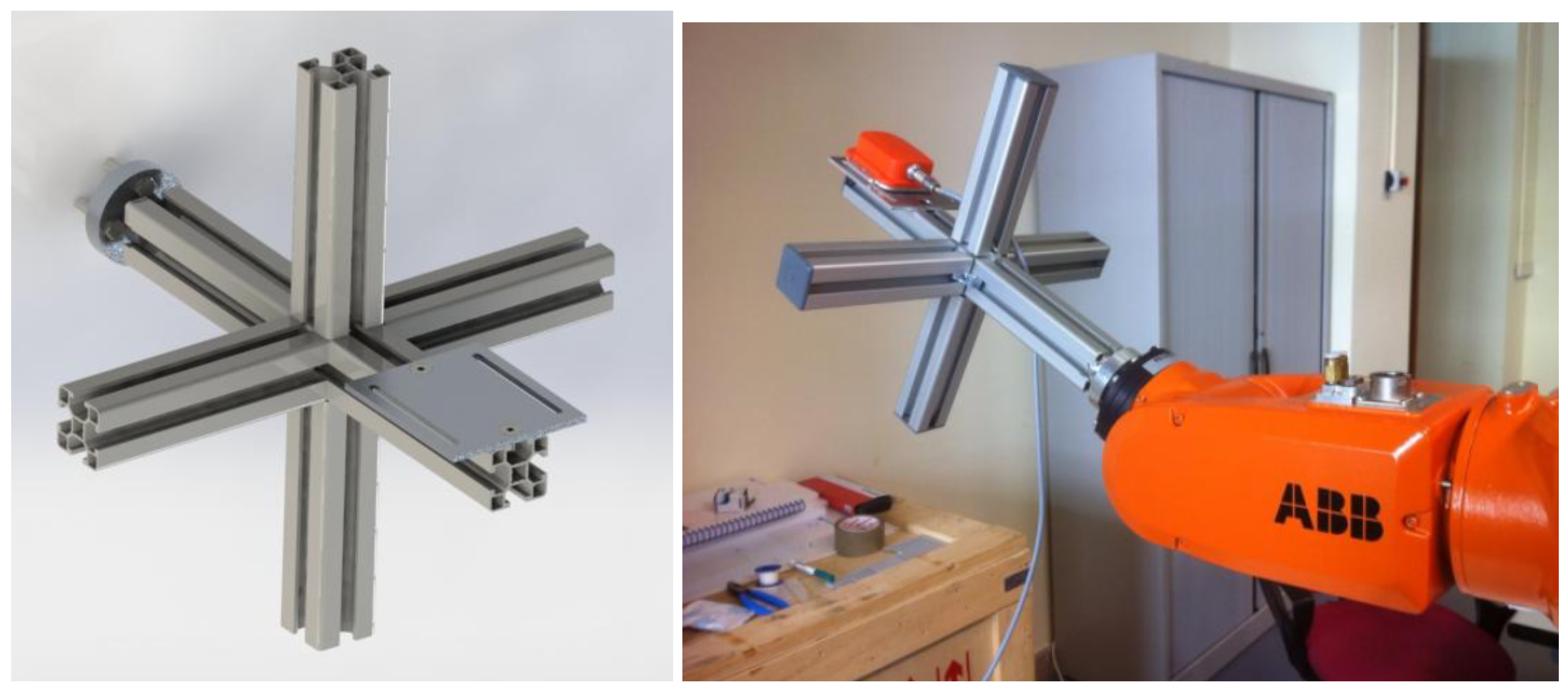
To evaluate and compare the estimation methods presented, a set of experiments was designed. Inertial sensors were attached to a robot arm programmed with a set of motions. The robot position was stored synchronized with the sensor readings. The data were processed with all methods, and their results were evaluated against the actual robot displacement, which provided the ground truth.
The robot was a six-degree-of-freedom industrial manipulator IRB-120 from ABB, reaching 580 mm with a maximum payload of 3 kg and a position repeatability of 0.01 mm. It was fixed to a workbench and previously calibrated. This robot provided a worst-case linear trajectory repeatability of 0.07 mm (a nominal maximum load of 3 kg and a linear motion with six axes at 1600 mm/s [
20]).
To calculate cyclical displacements in real-time for ambulatory applications, they have to be estimated in one stride or step time period. This time span, or integration time, is very short. For a wide population of 95% of healthy men and women, aged from 13 to 80, the step time in walking can be as long as 0.8 s (a cadence of 75 steps/min), and it can decrease to 0.4 s (cadence of 150 steps/min) when the walking velocity increases [
21]. This can occur at free-speed walking velocities in ranges approximately from 0.8 to 1.8 m/s.
Likewise, these parameters are subject to certain kinematic restrictions. For example, the stride length (SL) can be measured from the foot [
19] or from the antero-posterior displacement of the body center of mass (apCOM) [
17]. The average stride length (or two steps) increases with walking speed, varying in the interval of 94–185 cm for the same wide population and the same walking speed ranges mentioned previously [
21]. These motions are made with accelerations around 2–5 g [
22]. Likewise, trunk vertical excursion (vCOM) is known to increase with walking velocity, roughly from 2.2 to 6 cm at cadences between 66 to 120 steps/s [
23] or step times of 0.5–0.9 s. It is also reasonable to hypothesize that vCOM initial and final positions at every stride are the same, which makes its average velocity zero. Inversely, the COM medio-lateral displacement (mlCOM) decreases with walking velocity, in the range from 8 cm at 66 steps/s to 2.4 cm at 120 steps/s [
24]. All these variables affecting the estimation of displacements of interest in HMS are summarized in
Table 1, assuming a duration of a gait cycle (step) in the range of 0.4–0.8 s.
From these considerations, it is clear that the problem of MEMS-based distance estimations in human motion science is relevant for integration times from 0.4 s (a fast step time) to 1.6 s (a slow stride time). Within this time rank, motions of interest can be divided into two groups: short range motions of a few centimeters (COM-type) occurring at mean velocities between 1 to 20 cm/s, and large range motions (step-like) with mean velocities ranging between 60 and 230 cm/s. These numbers will be used to define eight experiments covering both types of kinematic conditions. experiments in similar kinematic ranges.
The robot was programmed to make eight types of linear vertical motion in the Cartesian space, which tries to resemble the previously discussed whole scenario of distance estimation in typical human motion applications, summarized in
Table 2. A short (4 cm) linear trajectory was executed at increasing speeds {1, 2.5, 5, and 10} cm/s. Similarly, a large (40 cm) trajectory was made with speeds of {10, 25, 50, and 100} cm/s. The short trajectory resembles the conditions of COM-like displacements, and the large trajectory of step-like (half the stride) displacements. Each experiment was repeated 50 times to provide statistical significance. The motion parameters were chosen also to provide the same four integration time scenarios in both trajectories, {4, 1.6, 0.8, and 0.4} s, relevant in the context of biomechanics, as discussed in the previous section. The motion was recorded with margins of 0.05 s before and after it was made, to clearly capture the whole motion, so the effective integration time applied was {4.1, 1.7, 0.9, and 0.5} s. In the case of the fastest motion 100 cm/s (Experiment 8), the integration time was incremented further to 0.625 s forced by the physical limitations of the robot. The Experiments 1 and 4 imply an integration time of
= 4.1 s, which is outside the scope out of the range of interest of this study. They will be used as a reference, to understand how the conclusions obtained for
under 2 s extrapolate to larger integration times.
A custom-designed end effector for the robot was used, which allows one to simultaneously test several accelerometer units, see
Figure 2. The units were rigidly attached to the end effector and statically calibrated. Individual calibration was performed with the sensor devices attached and at rest, in the middle point of the linear trajectory.
Three different accelerometers were tested simultaneously, and their nominal characteristics are synthesized in
Table 3. Their noise density
given by the manufacturer was taken as a first indication of the sensor quality. The Accel.XS is part of an MTi IMU device from Xsens
® with accelerometers from ADXL206 [
25,
26]. The Accel.LS is integrated in an IMU unit from Shimmer
® with a low-noise analog accelerometer Kionix model KXRB5-2042, which has a better noise performance than the previous model. The Accel.WR is a wide-range accelerometer also included in the previous device, with an LSM303DLHC digital accelerometer from STMicro with the highest nominal noise level of the three [
27].
In the three cases, the user can read the raw uncalibrated sensor data with a sampling frequency of Hz. However, the setup of the internal signal conditioning, the anti-aliasing filter, and the sampling by the dedicated CPUs are not always available, so it is difficult to know the effective sensor bandwidth . In the table, a reference value is given, as suggested by the IMU manufacturers and its corresponding RMS noise density level .
In our experiments, sensor data was recorded at the maximum sampling rate available,
or 512 Hz, depending on the device. Once the sensor was fixed to the end effector, an individual static calibration of its orientation was required. This reorientation was made with the TRIAD method, by using the magnetometer data with the robot at rest [
28]. The direction of earth gravitational and magnetic fields (global coordinates) were used to compute two measurements
in local coordinates, which were converted to a local triad
by the following process:
The same process was applied to calculate a global triad , and both of them allowed us to compute a re-orientation matrix . The gravitational field is much more robust and reliable than the magnetic field to be used as a measurement reference, and, for that reason, the robot moved precisely along the vertical axis, and the raw data was reorientated with matrix . No other data curation is done.
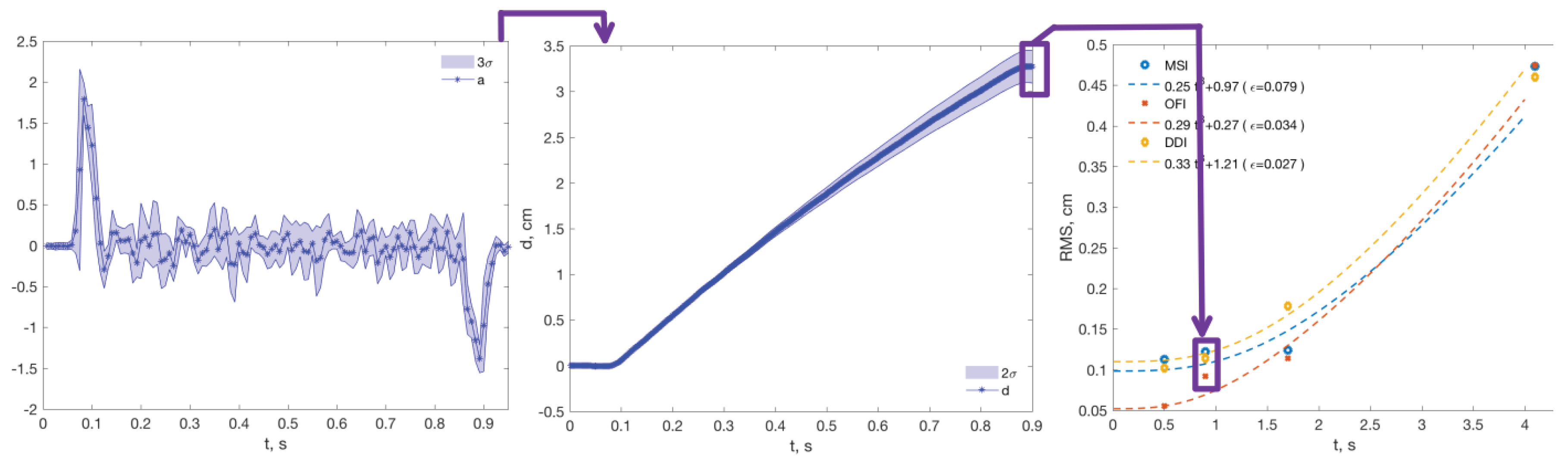
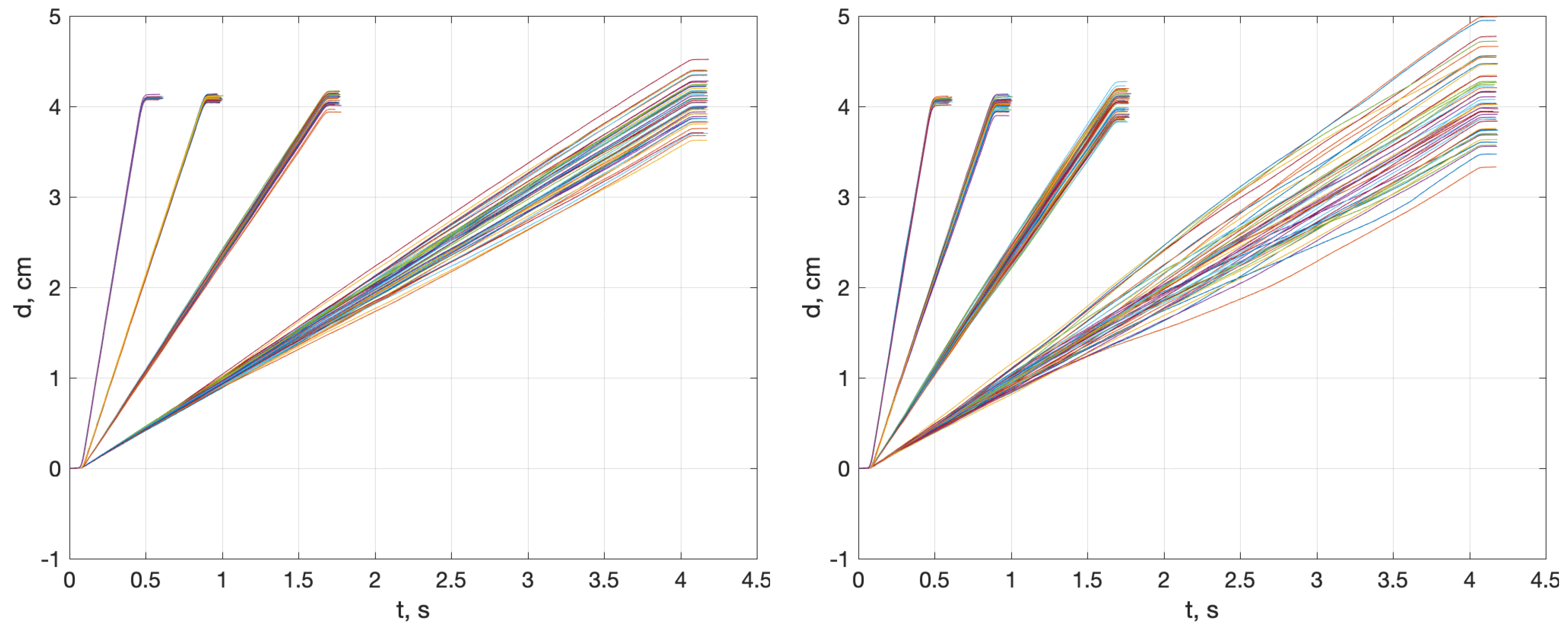
The controlled motion of the robot generated an acceleration profile that is similar in the eight experiments described in
Table 2. It started with a short acceleration peak, a long period of zero acceleration corresponding to the constant velocity motion, and an inverse symmetrical peak of deceleration to reach zero velocity again, see
Figure 3 Left.
Each of the eight experiments in
Table 2 was repeated a number of times
M = 50. The
M signal segments, sampled with frequency
, were stored and inspected to find artifacts that can occur if samples are lost during a repetition. This was the case for Accel.LS and Accel.WR when sampling at high frequencies (512 Hz). All the signals were inspected to remove those that were non-useful, leading to the discarding of six and seven in 400 repetitions, respectively.
Each of the valid
M blocks formed a data set, each having
N samples, accounting for
s, which corresponds to the integration time for the estimations. Within each block, the data were integrated to obtain a linear position with the five distance estimation methods in
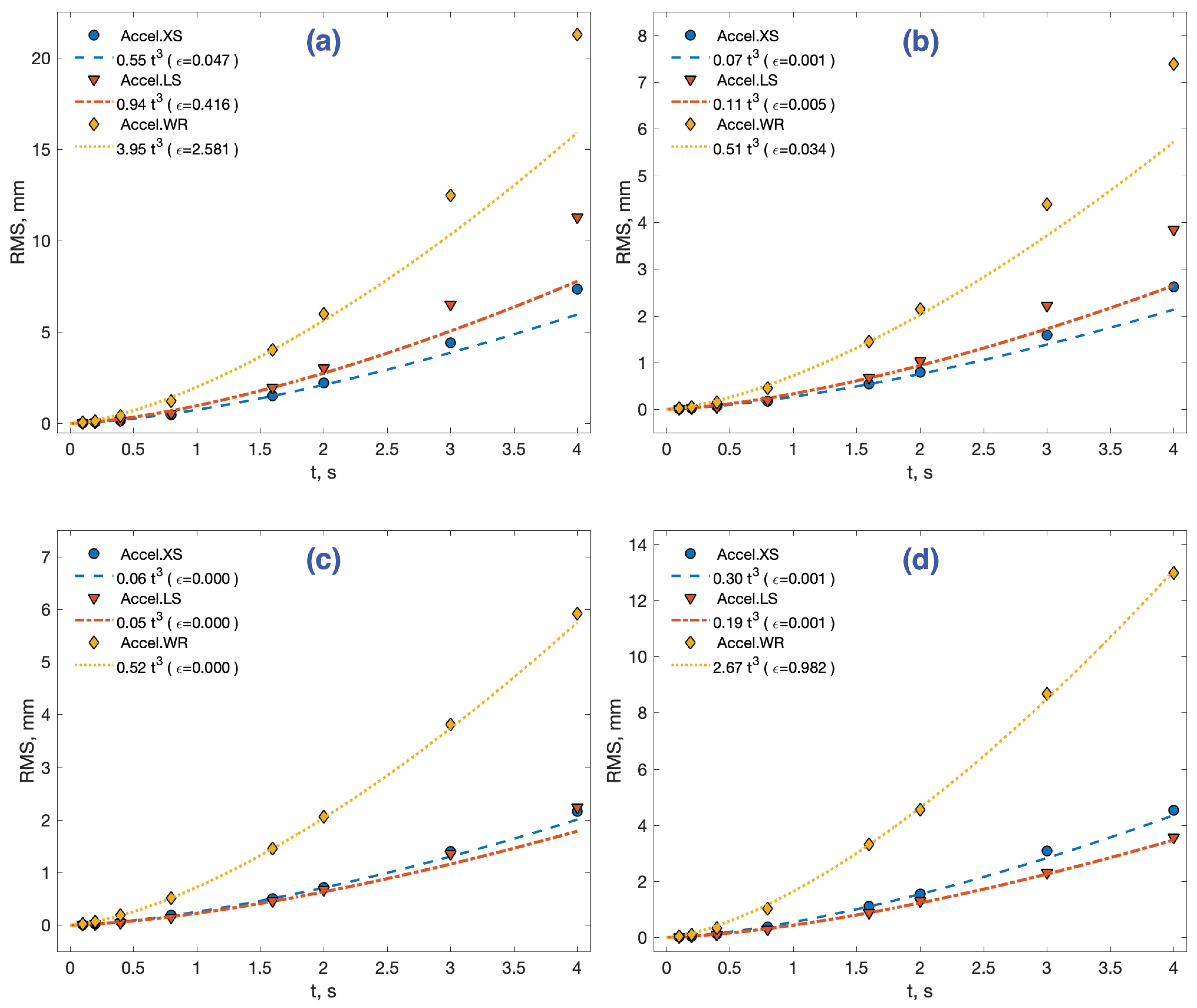
Table 4. The error in the last sample (Nth sample)
was calculated for each block
. Then, its root mean square error (RMS)
will be used to evaluate the response:
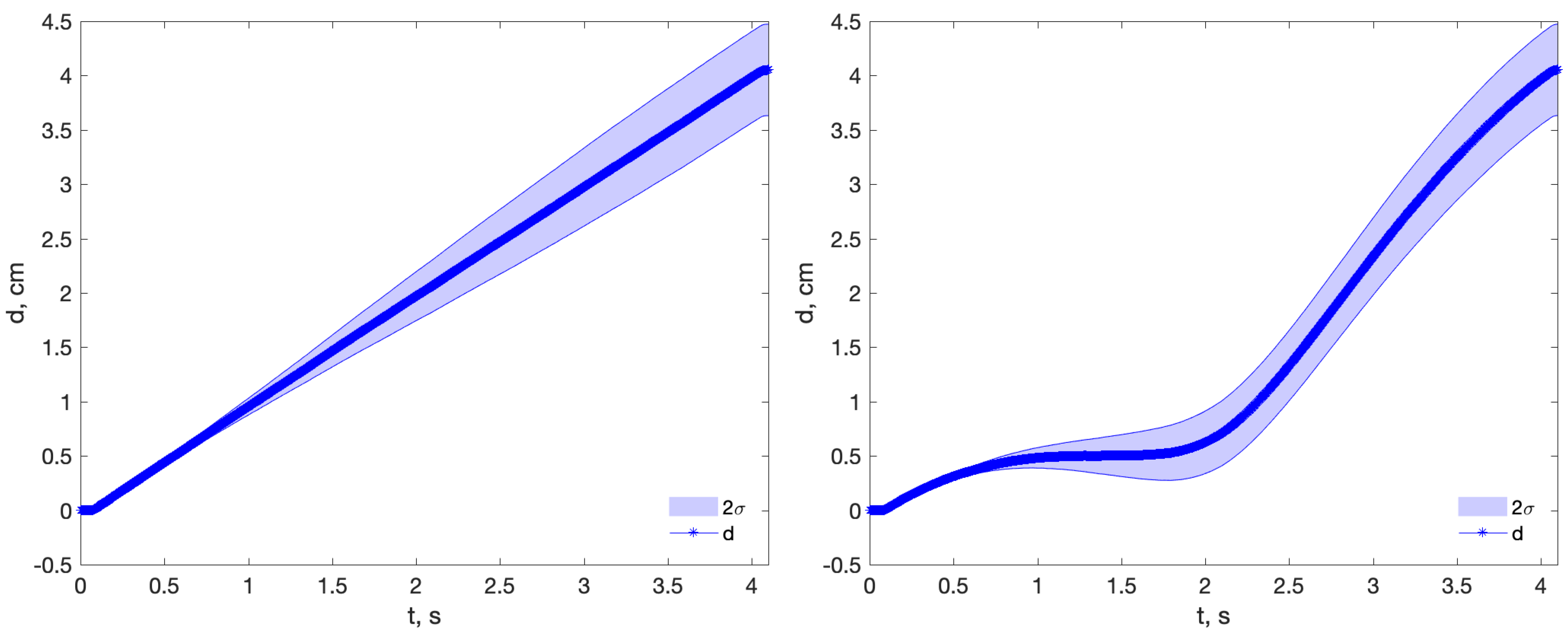
The complete methodology is represented in
Figure 3.
6. Conclusions
The measurement of distances using accelerometers is a functionality that is used in many HMS applications. The context of these measurements is an integration time of less than 2 s, and a movement length of up to 2 m. Even in these restricted conditions, it is advisable that the estimation algorithm incorporates some mechanism to limit the growth of the error, which, being quadratic in nature, deteriorates the estimates even for such small integration times.
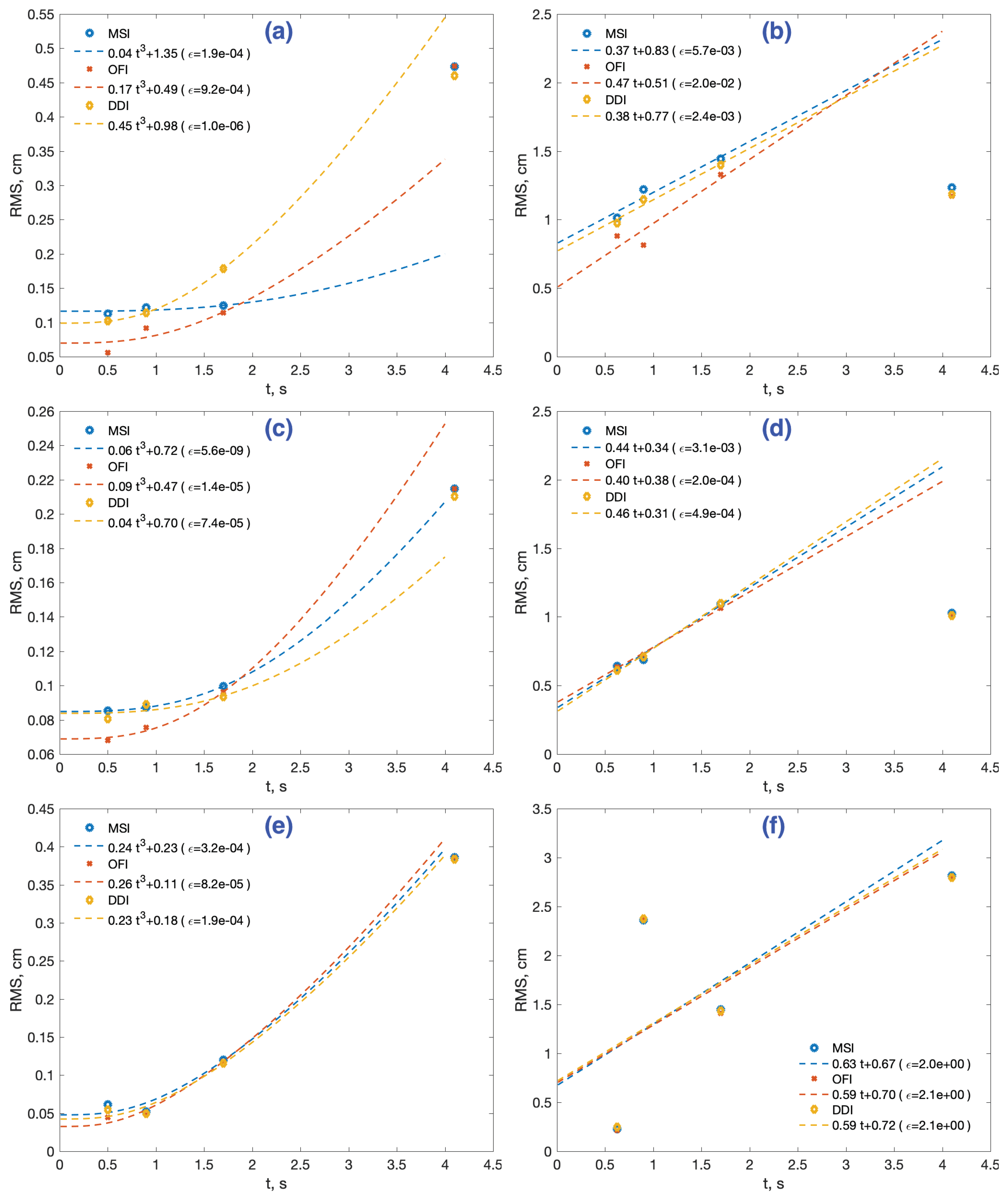
In this work, we have compared five methods with three different sensors in controlled experimental conditions, which reflect those found in practice in HMS. We have separated these conditions into two groups: short and long distances. The results obtained are as follows: (1) With the static sensor, the RMS error is related to the quality of the sensor in terms of bandwidth, noise density, and sampling frequency. The algorithms to reduce the error can reduce it by up to one-third. The simple elimination of the mean (MSI method) produces optimal results. The XS and LS sensors have a similar response, better than the WR. (2) With the sensor in motion, the expected error (RMS) in distance estimation is below 4.5% in 1.7 s for both distance ranges, whatever the sensor used. (3) The tested methods produce quite similar results in both groups of experiments. The OFI is sometimes better with low periods of integration, but no general rule can be defined in this respect. (4) The best sensor to estimate distances turns out to be the LS at all distances. For long distances and average velocities over 50 cm/s, the measurements are no longer reliable in all three devices.
The study confirms that it is feasible to use accelerometers to estimate short linear displacements of the body. More than the estimation method applied, the motion kinematic conditions can be a key factor in the performance of this estimation, combined with the type of accelerometer used, and those factors have to be jointly evaluated.


