1. Introduction
A core competence of geodesists is the profound knowledge of the stochastic properties of the measuring sensors used. This knowledge is essential to understand the influence of individual observations during parameter estimation, to detect outliers or to separate statistically significant deformations from the measurement uncertainty. TLS is currently playing a strong role in a wide range of applications including stability assessment [
1], bridge asset management [
2], and automatic computational model generation for historic buildings [
3]. However, the core competence mentioned at the beginning was ignored, since no stochastic model was available for more than a decade—neither from the manufacturers, nor from the side of academia. This circumstance is particularly surprising as an appropriate stochastic model is of vital importance for many important applications, e.g., the calibration of TLS [
4], the registration of point clouds [
5,
6] or direct georeferencing of TLS [
7,
8].
The frequently-used assumption of identical precision for all captured 3D points of a laser scan has already been disproved by several authors, e.g., by Schaer et al. [
9]. One of the first publications dealing with the analysis of systematic and random object influences on TLS measurements comes from Böhler et al. [
10], who showed a relationship between the reflectivity of the surface of the measured object and the noise of the measured distance. Elkhrachy and Niemeier [
11] introduced a distance-dependent stochastic model in the adjustment of transformation parameters. Several authors [
12,
13,
14,
15] performed studies on the influence of surface properties on the noise of distance measurements which were observed with terrestrial laser scanners. Soudarissanane et al. [
16] and Zámečníková et al. [
17] investigated the relationship between the incidence angle of the signal on the object surface and the absolute and relative accuracy of the distance measurement.
All these contributions were undeniably of great scientific importance, since they show individual aspects of the measurement uncertainty for individual points. However, it is not possible to establish the functional relationship for an all-embracing stochastic model considering all the aforementioned influencing factors. Even if this were possible, the necessary radiometric properties of the object surfaces are usually not known and would have to be modelled separately. Current research contributions by Wujanz et al. [
18] show an alternative approach in which the signal strength of the reflected measurement signal and the noise of the distance measurement are linked to derive a stochastic model. The validity of such an intensity-based stochastic model has been demonstrated in several investigations by Wujanz et al. [
18,
19] and was consequently used for various purposes by Cefalu et al. [
20] and Xu et al. [
21]. Ozendi et al. [
22] correctly stated that intensity-based stochastic models can only be used where raw intensity values in the measurement data can be accessed. Therefore, it is somewhat surprising that their own approach requires radiometric information and, consequently, is subject to the same restriction.
The reason why raw intensity values are suitable for stochastic modelling of reflectorless rangefinders can be justified by the radar range equation:
as given, e.g., by Wagner et al. [
23], which is not only valid for microwaves, but also for electro-magnetic signals with shorter wavelengths as explained by Höfle and Pfeifer [
24]. The parameters
Pe and
Pr denote the power of the emitted and received signals, respectively. The scanner’s receiver aperture diameter is represented by
Dr while
ηsystem signifies its transmission coefficient. Atmospheric influences are denoted by
ηatmos whereas the range between the scanner and object point is symbolised by
R. The angle of incidence is represented by
α, the quotient of reflection of the object’s surface in the wavelength of the scanner is described by
ρλ. In summary, all parameters in the equation have an immediate impact onto the received signal strength
Pr. From another perspective it can be concluded that all relevant parameters in (1) are inherently considered in
Pr which makes individual consideration of the influencing factors unnecessary and hence justifies the intensity-based method suggested by Wujanz et al. [
18].
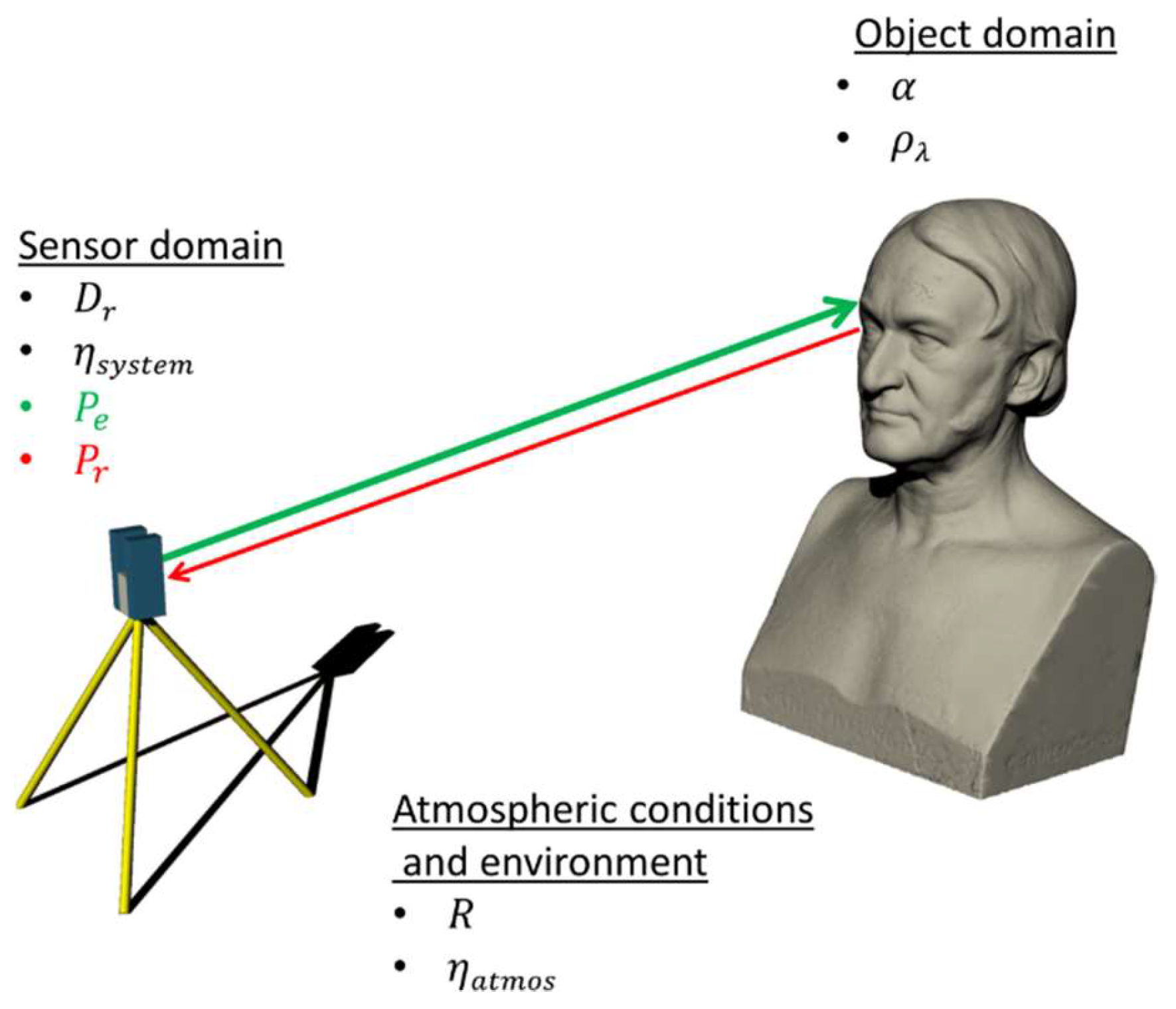
Figure 1 illustrates the scope of all factors which can be grouped in the following three main influencing factors:
- (i)
Sensor domain: In which an optical signal with the power Pe is emitted by a laser diode that is then deflected to the environment.
- (ii)
Environment: While travelling through the environment, the signal is subject to deterioration as a consequence of the range between scanner and an object’s surface as well as the atmospheric transmission coefficient ηatmos.
- (iii)
Object domain: On the object’s surface the signal is additionally weakened in dependence to the local quotient of reflection ρλ as well as the angle of incidence α. Another source which causes a loss of signal strength is provoked by the light collector of the scanner, as well as its deflection unit, that initiates the scanning process. The last two mentioned influences are summarised by ηsystem and are individual characteristics of the applied scanner that, hence, fall into to the sensor domain.
A restriction of the methodology proposed by Wujanz et al. [
18] is related to the necessity of repeatedly capturing ranges, which requires a deactivation of the scanner’s deflection unit. This functionality is usually prohibited due to health and safety regulations, especially regarding eye safety. Hence, the first research question of this contribution is dedicated to the search for alternative approaches in order to experimentally determine the stochastic properties of a terrestrial laser scanner’s rangefinder. Two novel methods are proposed in
Section 2 in order to derive intensity-based stochastic models based on capturing geometric primitives in the form of planar panels.
The second research focus is set on the transferability of intensity-based stochastic models and tries to clarify if these models are universally valid for all rangefinder types since, thus far, only TLS with phase-shift rangefinders were investigated. The basic principle of phase-shift rangefinders is explained, e.g., by Kahmen and Faig [
25] (p. 151ff) and Vosselman and Maas [
26] (p. 5ff). Lichti [
4] presented an extensive investigation of a laser scanner that applies this rangefinder technology. The transferability of intensity-based stochastic models is subject of
Section 3 where laser scanners with rangefinders that apply the impulse method as explained, e.g., by Kahmen and Faig [
25] (p. 150), which is often also referred to in the literature as the time-of-flight-principle (tof), e.g., by Vosselman and Maas [
26] (pp. 3ff), and hybrid rangefinders specified by Maar and Zogg [
27] that combine impulse and phase-shift approaches are analysed. A discussion about the findings of the contribution at hand can be found in
Section 4.
2. Determination of Intensity-Based Stochastic Models Based on Point Clouds
This section presents two methods for determining intensity-based stochastic models using planes. The planarity of the samples used is below the measuring precision of the applied laser scanner’s rangefinder and, therefore, does not affect the result. If this assumption does not hold, the imperfection of the applied plane would directly distort the computed stochastic measures. An important issue related to the generation of intensity-based stochastic models is that a potentially large range of intensity values should be acquired. This is of great importance in order to reliably capture the characteristic operation of the scanner’s stochastic behaviour. The run that describes the stochastic model is mainly influenced by the characteristics of the receiving photo diode as pointed out by Vosselmann and Maas [
26] (p. 14) and Mettenleiter et al. [
28] (p. 51ff) that derives the range between the scanner and object, as well as the signal’s strength based on the received signal.
Figure 2 shows the relevant intensity ranges on the abscissa axis and the associated measurement noise on the ordinate for a fictitious TLS. The red values indicate the usable range of the signal for the determination of an intensity-based stochastic model. The red curve approaches asymptotically to a black line, which shows the resolution of the rangefinder at high intensity values. In other words, the model does not allow drawing conclusions below the resolution of the rangefinder, since the measurements captured in this intensity region randomly differ by the amount of the resolution. As the intensity decreases, the noise increases and finally reaches the blue jagged area, in which correct range measurement is no longer possible. This region is caused by electronic noise yielding arbitrary ranges and consequently unpredictable range noise. Therefore, measurements captured in this region are consequently not considered for further processing.
2.1. Interpretation of Residuals as Rangefinder Stochastics
The general idea to interpret the residuals that emerge between a planar target and acquired observations as stochastic properties of a reflectorless rangefinder is, per se, not a novel idea (see, e.g., Böhler et al. [
10]). Ozendi et al. [
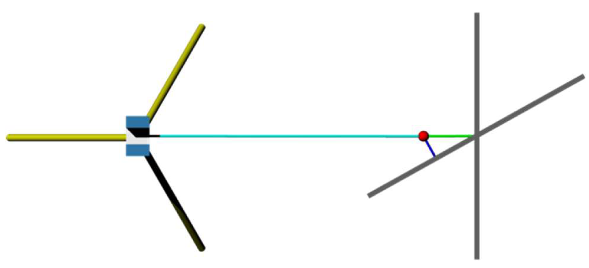
29] applied this approach, among others, and set the range noise of a TLS in relation to intensity, object distance, as well as the angle of incidence. The latter aspect has to be seen quite critical as the noise of a captured range is correlated to the direction from where it has been observed. Since the residuals of a plane are bound to its normal direction an increasing rotation of a planar target in relation to a TLS would decrease the magnitude of the resulting residuals. Soudarissanane et al. [
30] avoid this falsifying impact by considering the observational direction for every point.
Figure 3 illustrates the aforementioned circumstance where a distance to a plane is observed under two incidence angles. Note that for illustrative reasons the range noise is assumed to be equal for both scenarios. The resulting point is highlighted by a red circle. It is obvious that the green tinted residual that runs parallel to the observational direction (highlighted by a cyan coloured line), is larger than the blue one which is associated to the face normal of the tilted plane. In essence, this means that the derived range noise is dependent on the orientation of the observed plane. Lambertus et al. [
31] noticed and verified this effect within laborious experiments conducted with a time-of-flight scanner, specifically the Leica ScanStation C10. Furthermore Lambertus et al. [
31] adapted the idea of linking the signal strength to the arising noise within point clouds. Interestingly, the results show similar characteristics to the findings of Wujanz et al. [
18], who applied this to the data from a phase-shift scanner.
A vital aspect which has not received adequate consideration in the context of stochastic modelling of reflectorless rangefinders is the validity of the outcome. This issue will be of particular interest in
Section 2.3 where results generated by repeated range measurements are compared against outcomes computed based on the two introduced procedures presented in this subsection as well as
Section 2.2. The first experiment included data acquisition of four planar samples with sizes of 50 by 50 cm at different ranges with a Zoller + Fröhlich IMAGER 5006h (Zoller & Fröhlich GmbH, , Wangen im Allgäu, Germany). A GOM ATOS I (GOM GmbH, Brunswick, Germany) structured light scanner was used to verify the planarity of the samples. This adds up to ~0.1 mm and, hence, falls into the range of the applied scanner’s resolution [
32]. Every sample features different radiometric properties ranging from black to white. By this, a large spectrum of different intensity values should emerge based on a comparably small set of object distances.
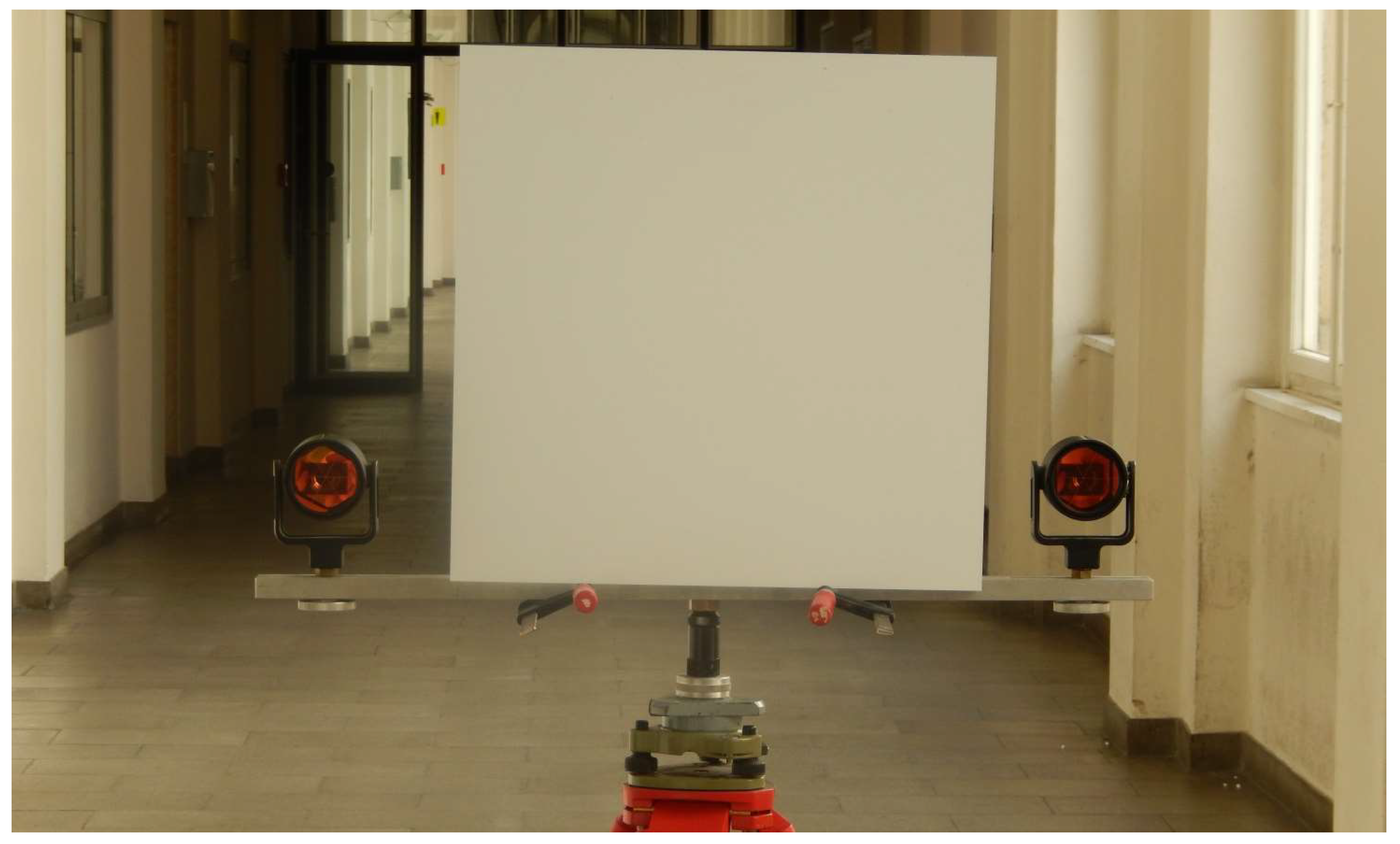
In total, eight viewpoints with ranges between 5 and 56 m in approximately 6 m increments were observed. At every position four radiometrically different samples were recorded. In order to ensure incidence angles that are nearly parallel to the face normal of a planar sample a mount has been used that is illustrated in
Figure 4. The alignment of the mount and, hence, the sample is conducted by using a total station that is fixed to the scanner’s tripod under forced centring and two prisms on the mount. Data acquisition was performed under fixed settings with the resolution setting “ultra high” corresponding to an angular increment of 0.009° and the quality setting “high”. A disadvantage of applying fixed angular settings is that the point sampling captured at different object ranges varies notably. However, this was necessary due to the fact that the sampling rate for Z + F scanners is bound to the aforementioned settings as explained by Mettenleiter et al. [
28] (p. 66). Altering these settings would, in turn, change the measurement rate of the rangefinder and thus yield in a notable change of the range noise. Ultimately, a mixture of various noise levels would lead to an inhomogeneous basis for stochastic modelling.
In total 64 datasets were captured. By deploying a least squares adjustment the unknown plane parameters and, finally, the residuals
v were determined. In contrast to Wujanz et al. [
18] all observations received equal weights.
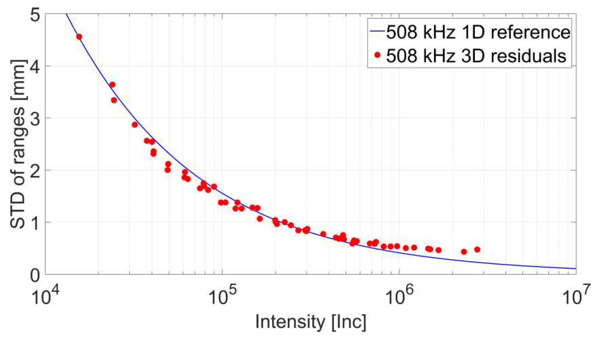
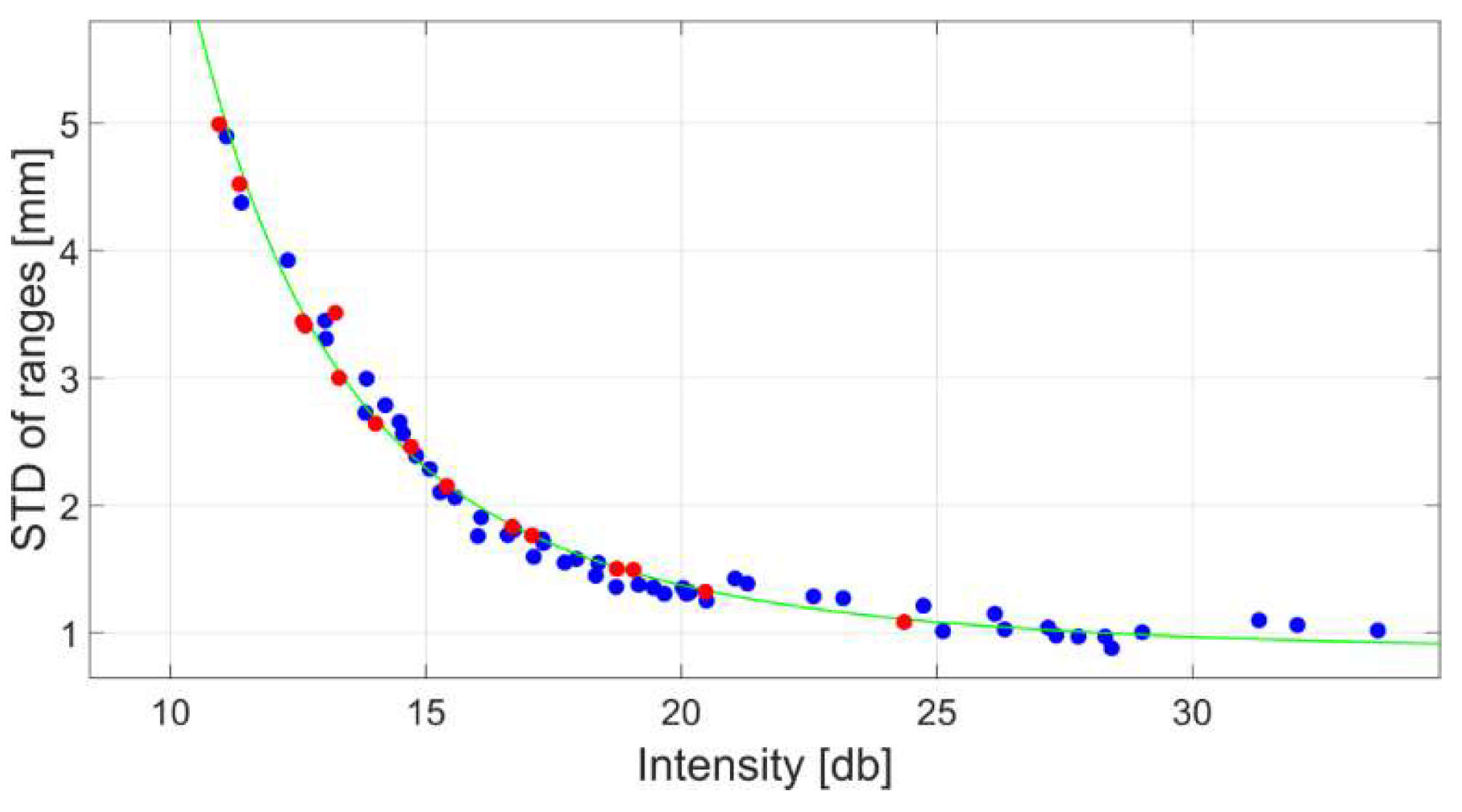
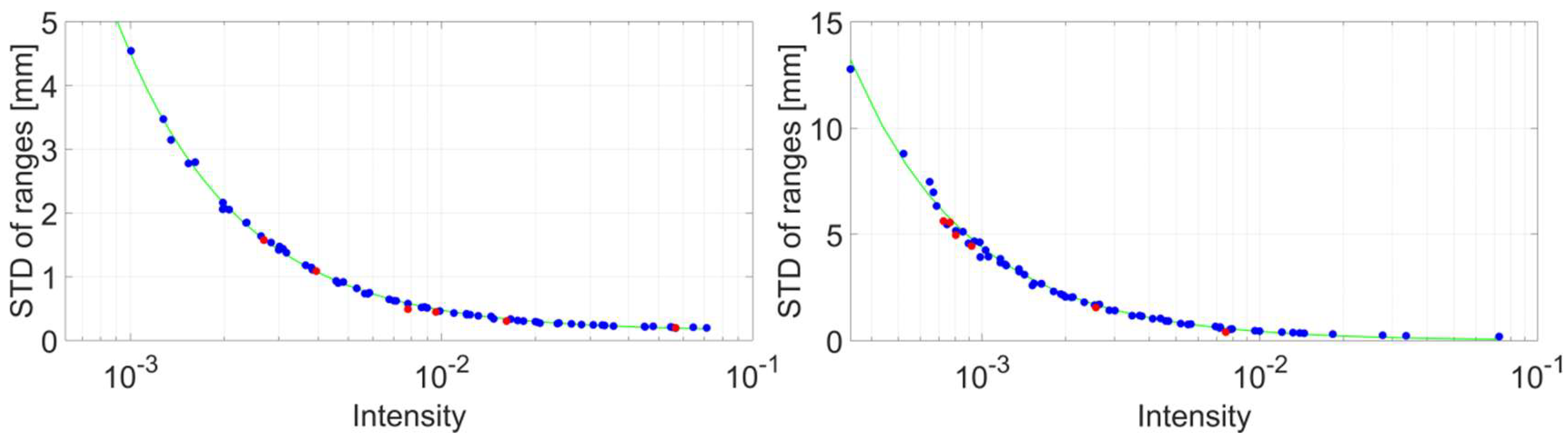
Figure 5 depicts the computed results that are highlighted by red circles. The standard deviation of ranges is graphed on the vertical axis while the raw intensity values can be found on the horizontal axis. The blue line represents the stochastic reference model generated by repeated range observations for a sampling rate of 508 kHz [
18]. While the computed stochastic measures largely comply with the reference run, differences in the magnitude of up to 0.17 mm can be spotted for higher intensity values. The reason for this characteristic is likely to be caused by larger changes of the incidence angle for panels acquired at close range as opposed to large object distances. A solution to this problem could be to restrict the incidence angle of points on a sample to a certain range.
2.2. Rangefinder Stochastics Based on Quasi-Ranges
A disadvantage of the procedure described in the previous subsection is linked to the dependence of the computed range noise to the angle encoders. In order to avoid this potentially falsifying effect, an alternative method to generate stochastic measures for a TLS rangefinder is proposed. The general idea behind this approach is to compute the range stochastics solely based on the recorded distances. In order to achieve this, the control software of the applied TLS has to offer an export function that includes the originally-observed polar elements direction φ, tilt angle θ, and range ρ, as well as the recorded raw intensity. For the applied scanner’s control software LaserControl an export option that includes all of the aforementioned elements is available. Therefore, the asc-suffix has to be chosen (Range/intensity as ASCII (uncalibrated)). Instead of using point clouds that describe the entire surface of the planar test sample, patches, of varying size are observed.
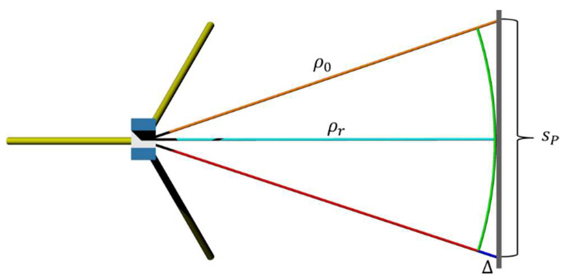
The reason for this is illustrated in
Figure 6 where a planar sample with a length of
sp, represented by a grey line on the right, is captured by a TLS. A representative range
ρr is tinted in cyan for which stochastic properties should be computed. The observed range
ρo is represented by the orange line. The green coloured semi-circle has a radius of
ρr. It can be seen that the discrepancy Δ between semi-circle and planar sample, highlighted by a blue line, increases towards the boundaries of the sample. Due to this effect differently sized regions have to be acquired in dependence to the object distance and the resolution/precision of the applied TLS’ rangefinder. Note that this geometrically provoked effect decreases with increasing object distance. However, if the entire sampled area would be considered, the resulting stochastic characteristics would increase as a consequence. Due to the fact that all captured ranges for a certain configuration are slightly different, the term “quasi-range” is used throughout the remainder of the paper.
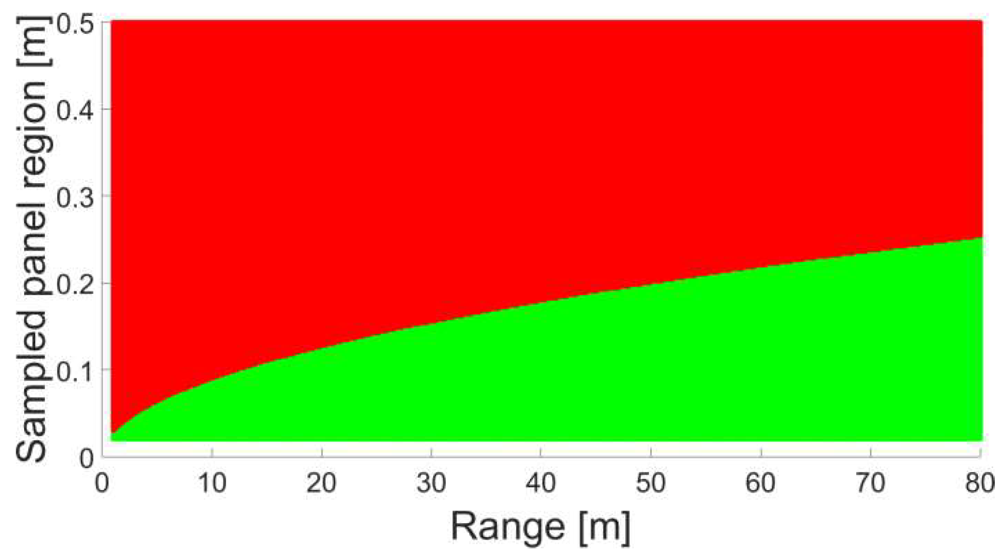
The mentioned problem caused by the proposed survey configuration can be tackled by scanning only a restricted region on the sample. In order to determine the expansion of this patch in dependence to the object distance some numerical investigations were undertaken. Therefore, the discrepancy Δ is computed by:
where
SP denotes the extent of the sampled panel region. Discrepancies Δ larger than the range resolution of the applied laser scanner are assumed to cause erroneous results and are, hence, omitted. For the applied TLS the resolution sums up to ~0.1 mm [
32].
Figure 7 illustrates the computed results where the range between scanner and sample is graphed on the horizontal axis. The vertical axis features the maximum extent of the area under consideration. Red tinted areas in the figure represent configurations where Δ exceeds the resolution of the scanner. As a consequence the corresponding range stochastics would be falsified. Green regions highlight combinations that are suitable to compute the stochastic behaviour of reflectorless rangefinders. It can be seen that the acquirable area on the panel increases with rising range.
Based on the considerations depicted in
Figure 7, a stochastic model has been generated by deploying the quasi-range procedure. Therefore, the same captured data has been used yet new input files were exported and cut to the corresponding maximum extent of the sampled panel region. Based on this information the standard deviation for ranges has been computed and graphed against the average intensity as illustrated in
Figure 8. Again the reference is highlighted by a blue line while red circles denote the outcome of the quasi-range method. Similar to the findings presented in the previous subsection both datasets coincide quite well for lower intensities yet drift notably apart with increasing strength of the recorded signal. In comparison to
Figure 5 the difference between reference and results generated based on the quasi-range method is notably larger. In addition, the run of the computed points is a lot noisier than the outcome presented in
Section 2.1. Thus, the conclusion can be drawn that the quasi-range method is quite delicate against an imperfection of the survey configuration in the form of a relative rotation between the scanner and the sample.
2.3.Evaluation of the Proposed Procedures
Based on the generated results depicted in
Figure 5 and
Figure 8 two intensity-based stochastic models were derived. Therefore the following functional model:
was used. The three unknown parameters
a,
b, and
c can be determined from a least squares adjustment considering the raw intensities
Inc. as observations and the values for the standard deviations
σρ as fixed parameters. Thus, Equation (3) will later on form the stochastic model for the precision of ranges
σρ.
Table 1 contains a comparison among a reference model against the parameters which were derived in
Section 2.1 and
Section 2.2. The reference stems from Wujanz et al. [
18] and was captured by repeated observation of ranges at a sampling rate of 508 kHz. Note that it is vital to introduce raw intensity values into the estimated functions that report the precision for ranges in metres.
In order to prove the validity of the generated stochastic model a procedure suggested by Wujanz et al. [
18] is used. The basic concept is in accordance to the overall model test of an adjustment as explained e.g., by Teunissen [
33] (p. 93) which decides if both, the functional and the stochastic model, are appropriate but also if potential outliers are within a given set of data. In order to validate the outcome of the adjustment, the following information is required:
observations that were captured with the TLS under investigation;
a functional model that is capable to represent the recorded data; and
a stochastic model that describes the precision of the measurements.
The observations that serve as input of the procedure are scans of planar shapes captured under randomly chosen survey configuration and radiometric properties. It is vital that the measurements are independent from the datasets that were used to derive the stochastic model. Under the assumption that a suitable functional model has been chosen and that no or negligibly few outliers are among the observations, it can be checked if the proposed stochastic model is appropriate. Therefore the empirical reference standard deviation:
is computed and compared against the standard deviation of the unit weight
σ0, which is also referred to as theoretical reference standard deviation. The sum of weighted squared residuals Ω can also be expressed in matrix notation where
v denotes the residual vector and
P the weight matrix of the observations. The value
f describes the degrees of freedom of the stated adjustment problem. The stochastic model is regarded as being appropriate if the empirical standard deviation
s0 falls into the interval of 0.7 <
s0 < 1.3 under the assumption that the standard deviation of the unit weight
σ0 was set to 1 as proposed, e.g., by Müller et al. [
34] (p. 345).
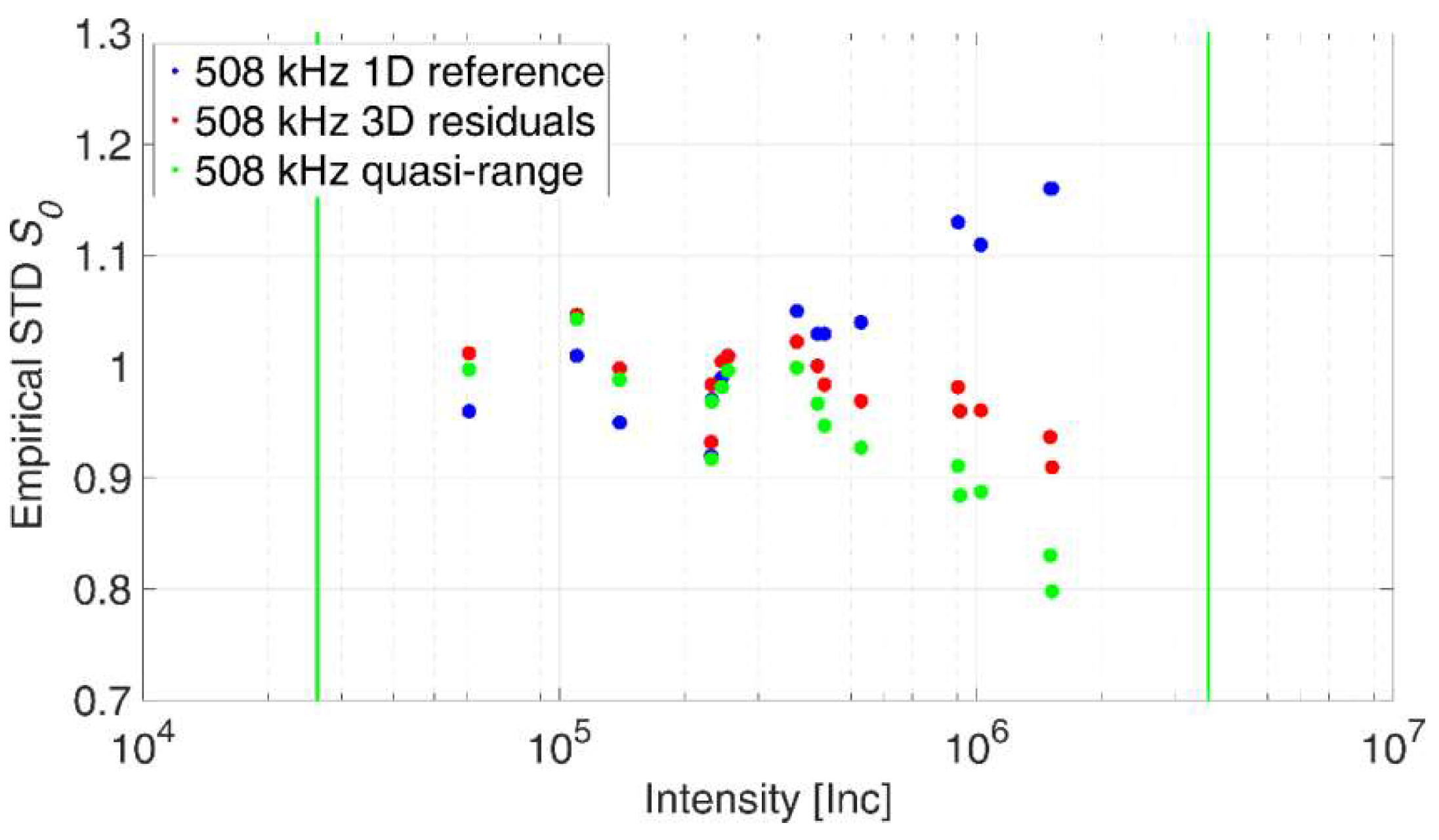
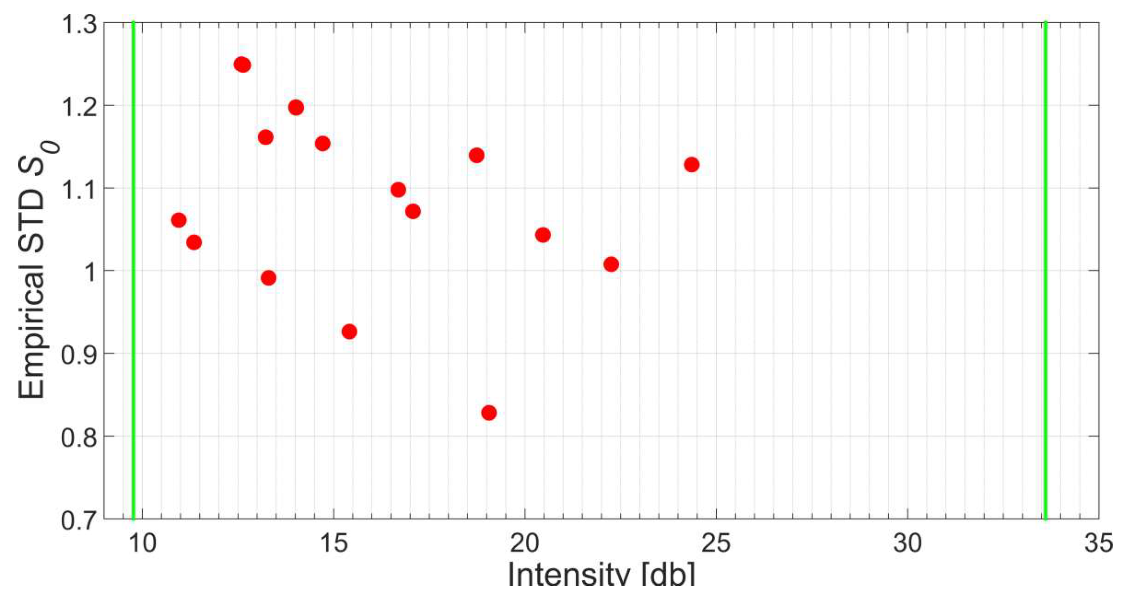
Figure 9 illustrates the results of the verification process. Therefore, 16 datasets from Wujanz et al. [
18] were used featuring planar panels that were captured under random survey configurations and varying radiometric properties. The corresponding data was then processed in a least squares adjustment using three different stochastic models yielding in different weights for individual ranges and, consequently, different empirical standard deviations
s0. The horizontal axis shows intensity values on a logarithmic scale. The vertical green lines highlight the smallest and largest intensity values that were captured in the experiments for the generation of the stochastic models. The vertical axis graphs the empirical standard deviations
s0 that stem from the plane adjustments.
The first model was generated based on repetitive range measurements according to Wujanz et al. [
18] while the corresponding results are depicted by blue circles. For the red circles the stochastic model generated in
Section 2.1 was used, while the green circles stem from
Section 2.2. All green and red circles fall into the specified interval of 0.7 <
s0 < 1.3. Hence, this outcome verifies the two suggested procedures for the generation of intensity-based stochastic models based on capturing 3D-point clouds instead of repeated range measurements. Note that the empirical standard deviations drift apart for higher intensities while a higher degree of conformity was apparent for the remaining parts.
4. Conclusions
This article demonstrates the circumstance, at first, that intensity values captured by terrestrial laser scanners inherently consider influences provoked by the survey configuration, the radiometric properties of a scanned surface, meteorological effects, as well as scanner-specific characteristics. Hence, intensity values are, per se, an appropriate input for all-embracing stochastic models of reflectorless rangefinders deployed, e.g., in terrestrial laser scanners. The suggested methodology does not require individual consideration of the influencing parameters—a course of action that is doomed to fail, as shown in
Section 1. A clear disadvantage of the initial procedure proposed by Wujanz et al. [
18] is its dependence to operate the rangefinder of the scanner under investigation in 1D-mode, a functionality that is usually prohibited due to health and safety regulations. In order to allow the generation of intensity-based stochastic models with TLS in normal operation (3D-mode) two novel approaches were suggested that are based on capturing planar shapes utilising 3D-point clouds. The final research question focussed on the universal validity of intensity-based stochastic models for all rangefinder types. While previous research by Wujanz et al. [
18,
19] exclusively investigated laser scanners that incorporate phase-based rangefinders, a Riegl VZ-400i impulse scanner, as well as a Leica ScanStation P40, that applies a hybrid rangefinder strategy, were investigated in this contribution. Since the stochastic characteristics of these laser scanners can also be described by intensity-based stochastic models, their generality was assured. In order to allow spreading the idea of intensity-based stochastic models into practice, it is desirable that some manufacturers offer the possibility to export unprocessed intensity values—a rather simple demand which, however, is only offered by very few companies. Prospective research will focus on ambient influences onto terrestrial laser scanners, as well as on configurations that yield the systematic biases of the rangefinder.

 ,
, 


