A Multiple Target Positioning and Tracking System Behind Brick-Concrete Walls Using Multiple Monostatic IR-UWB Radars


Abstract
:1. Introduction
2. Through-Wall Radar System
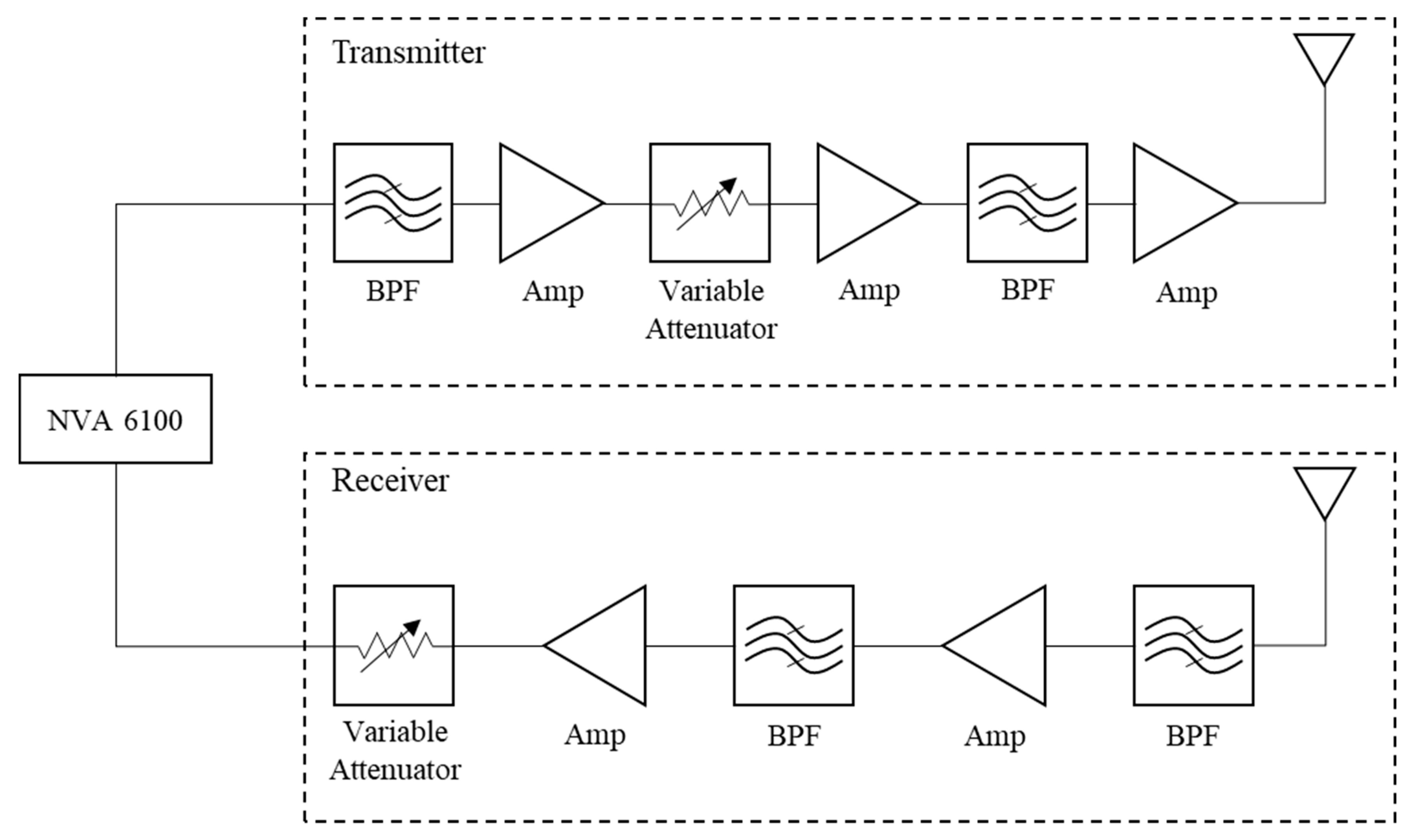
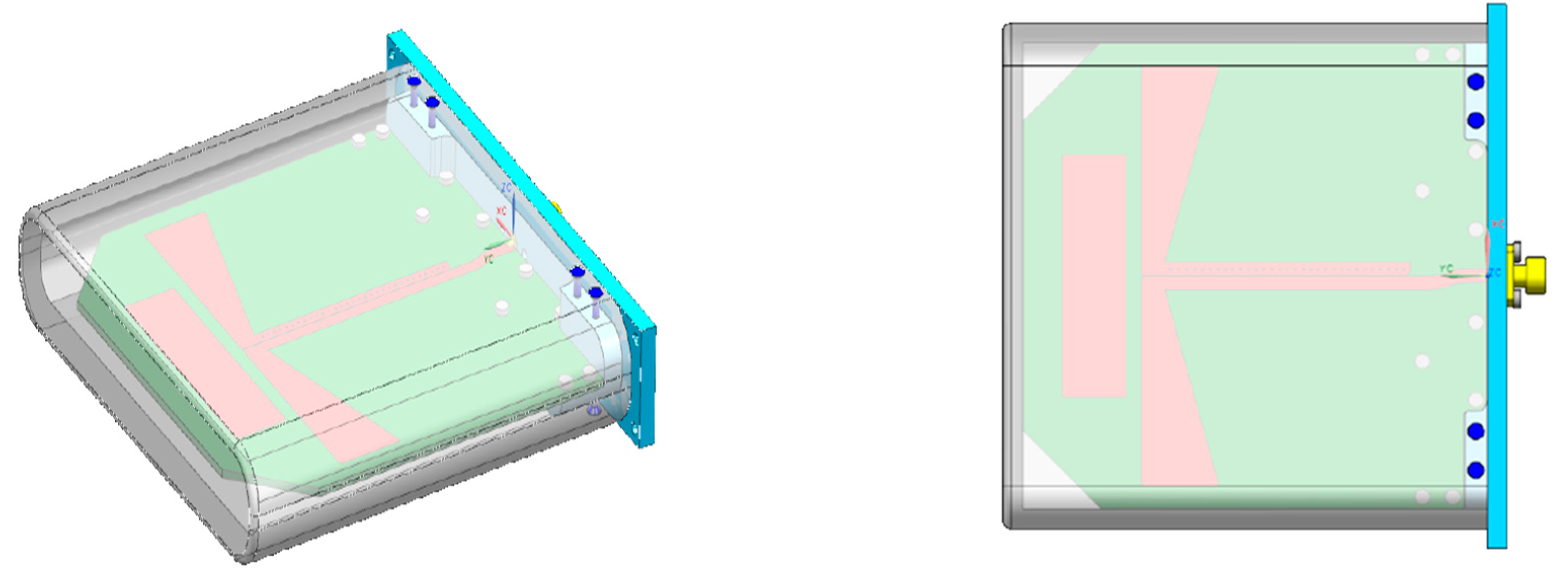
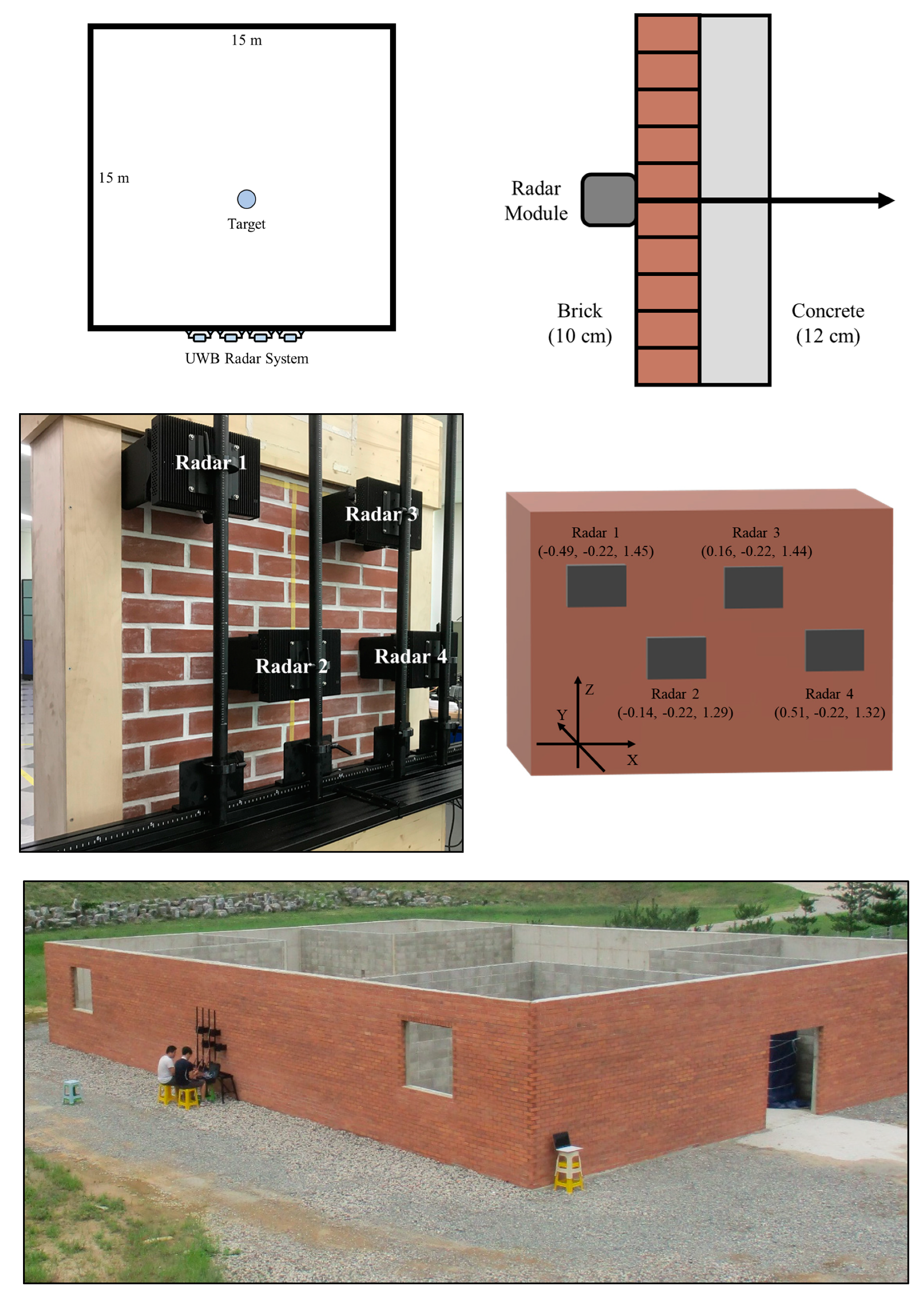
2.1. Hardware Design
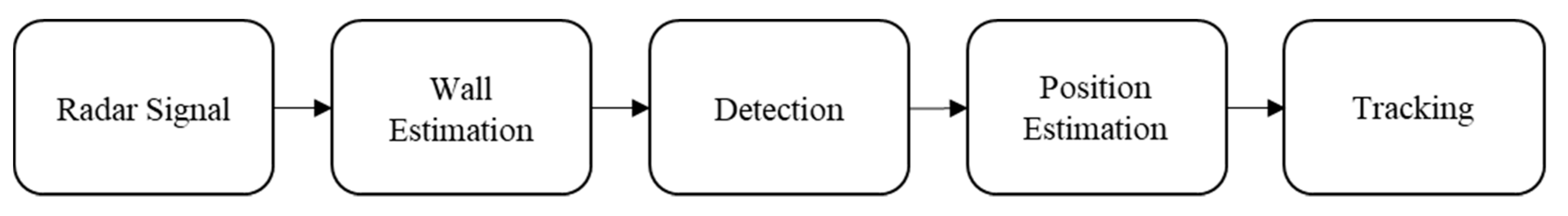
2.2. Through-Wall Radar System Process
3. Positioning Algorithm
3.1. Trilateration Algorithm
3.2. Delay-and-Sum Algorithm
3.3. Proposed Algorithm
| Algorithm 1 Position Estimation with the Proposed Algorithm |
| 1. Initialization Generate grids for and , considering the coverage and performance of the radar system. For example, in our radar system, one grid is a square of 0.2. 2. For and , calculate the cumulative likelihood as follows: 3. For and , normalize the cumulative likelihood for recursive operation as follows: 4. Find the coordinates over the threshold to estimate the location of multiple targets such that 5. Calculate the effectivity of grids as follows: |
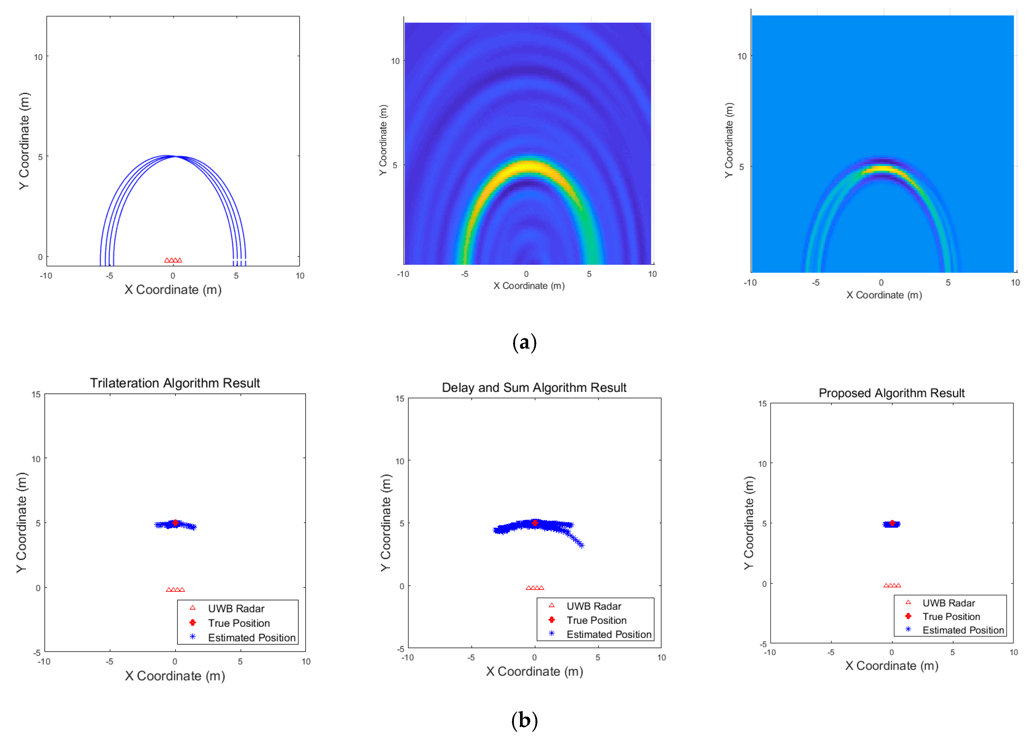
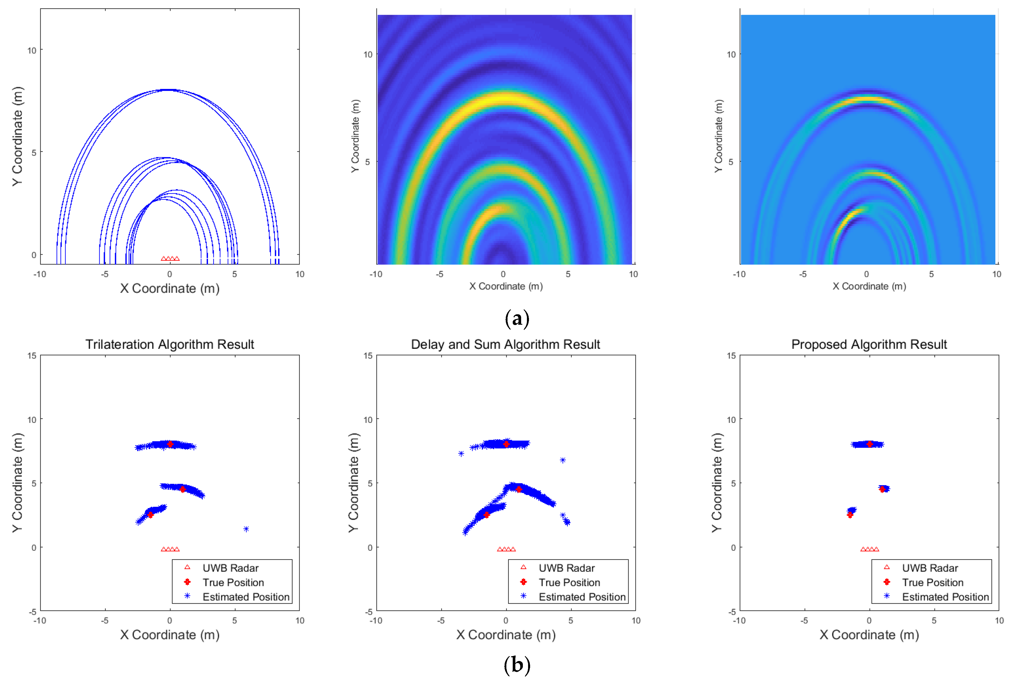
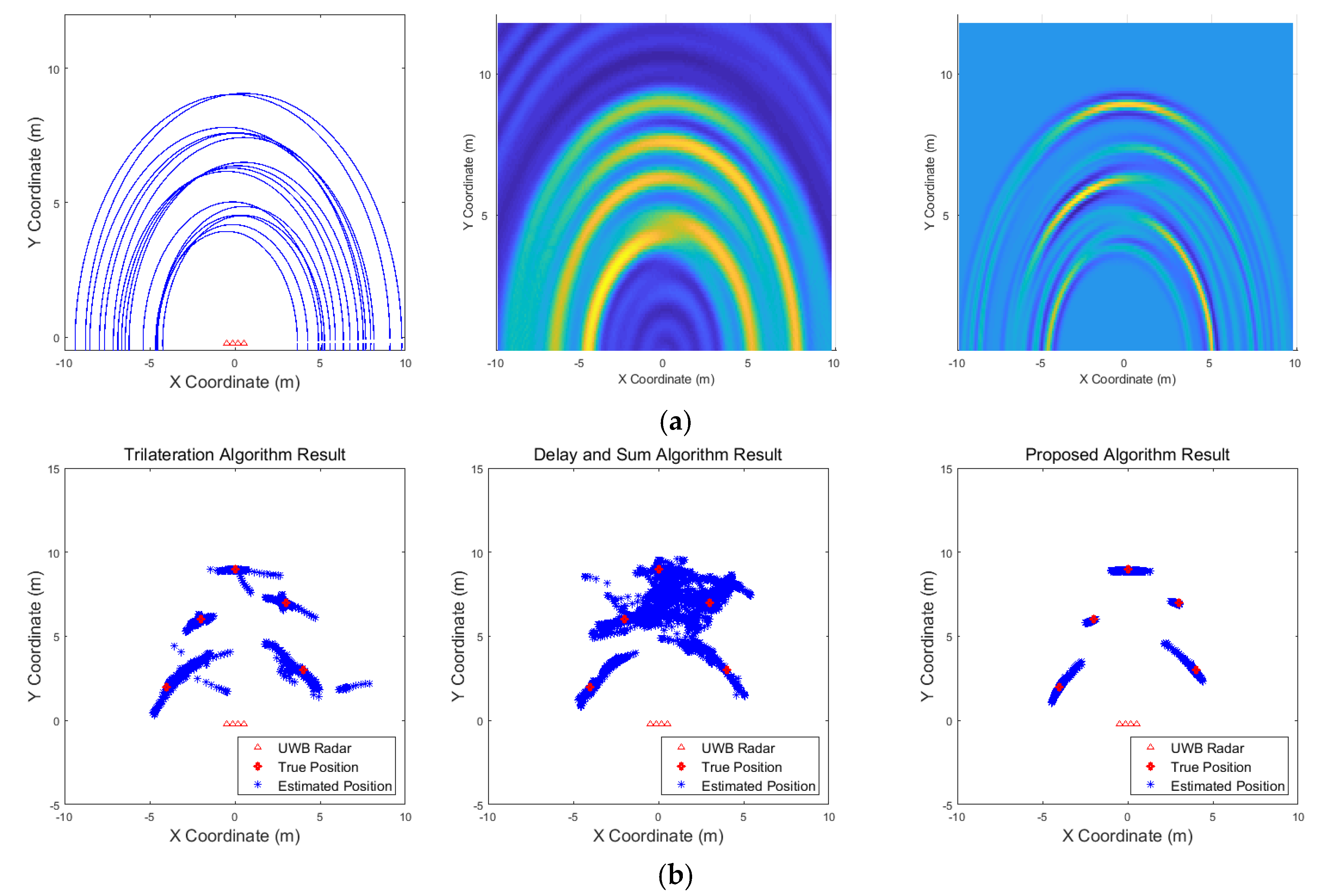
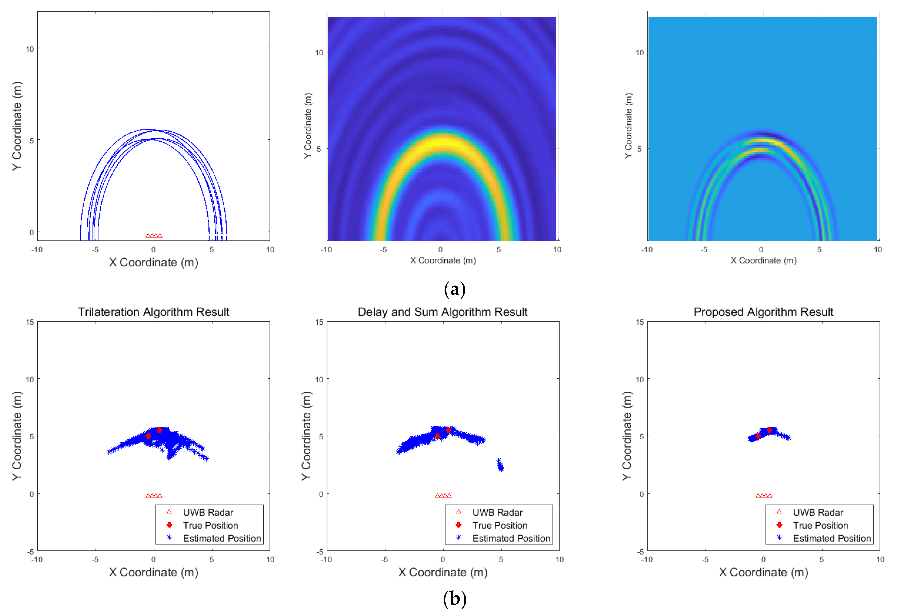
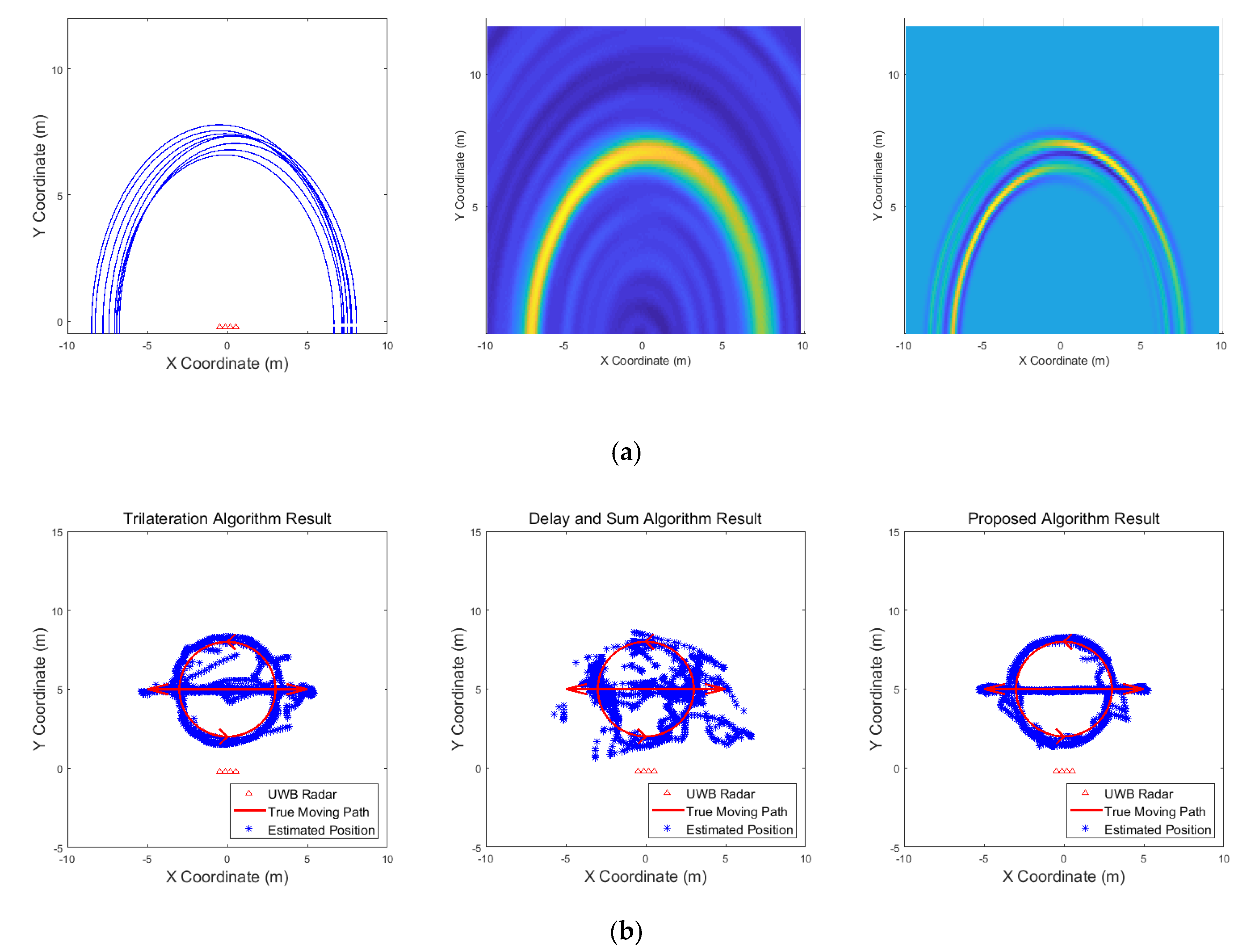
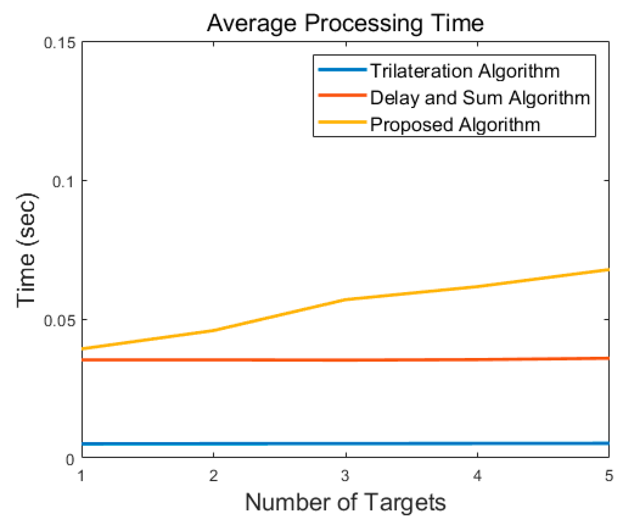
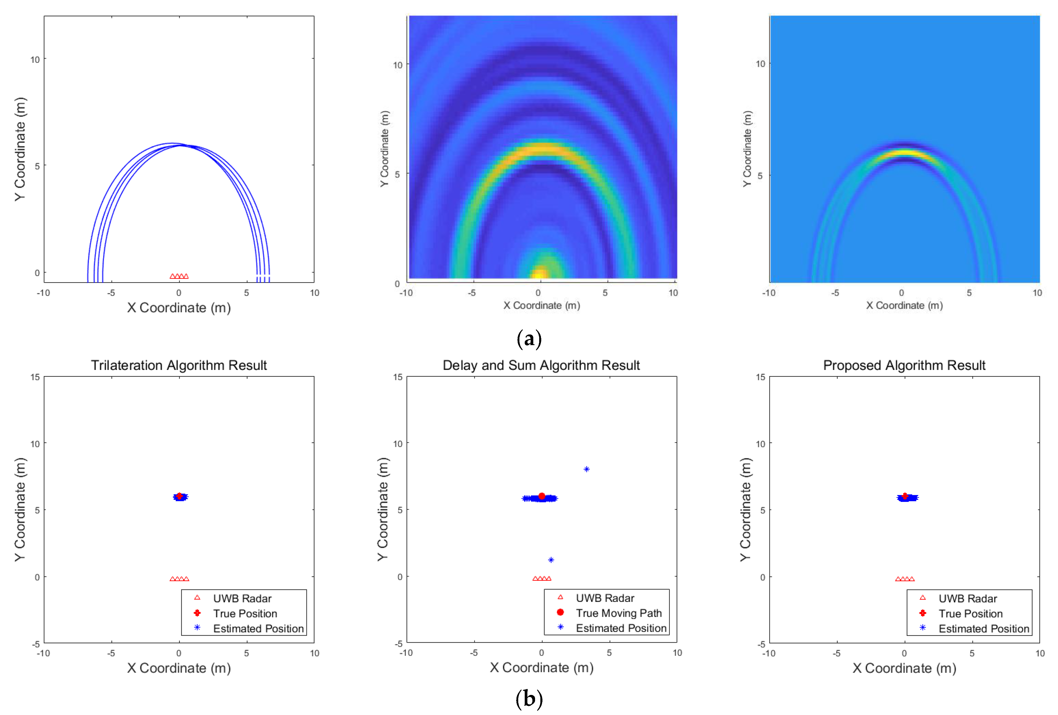
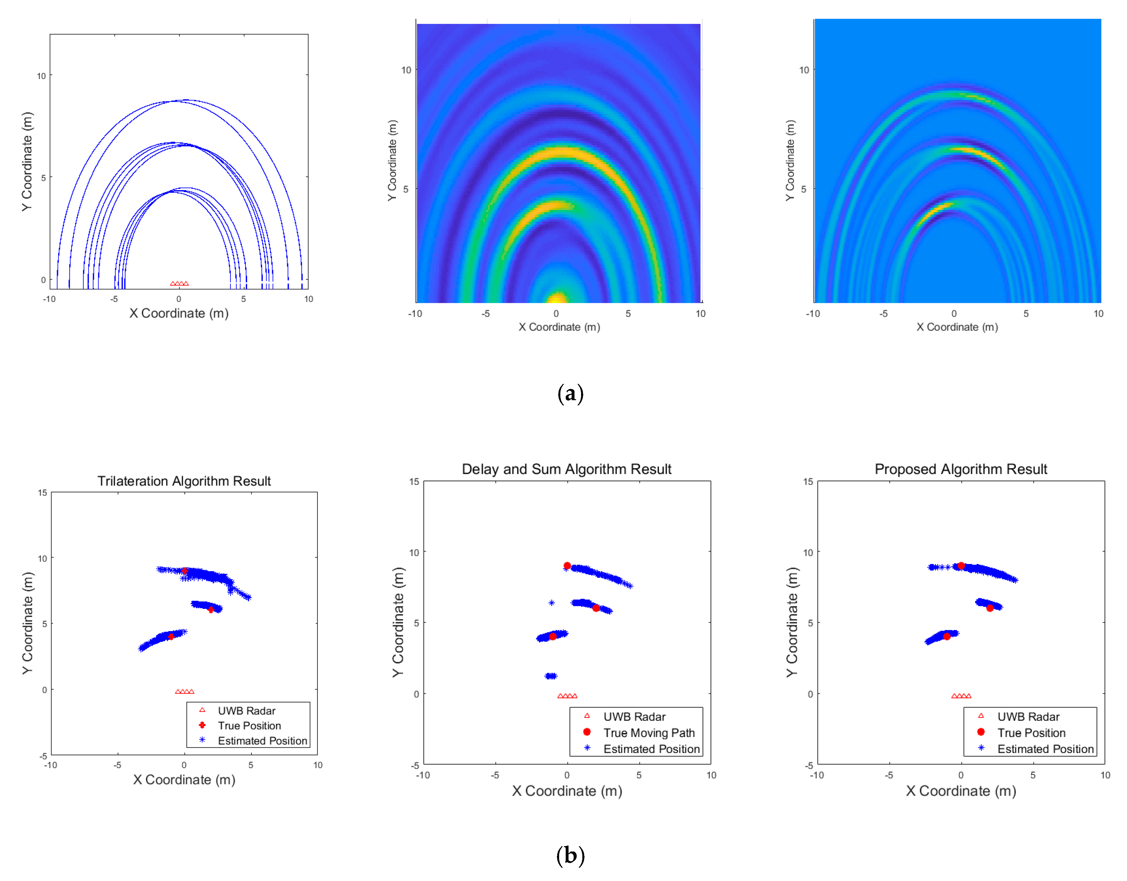
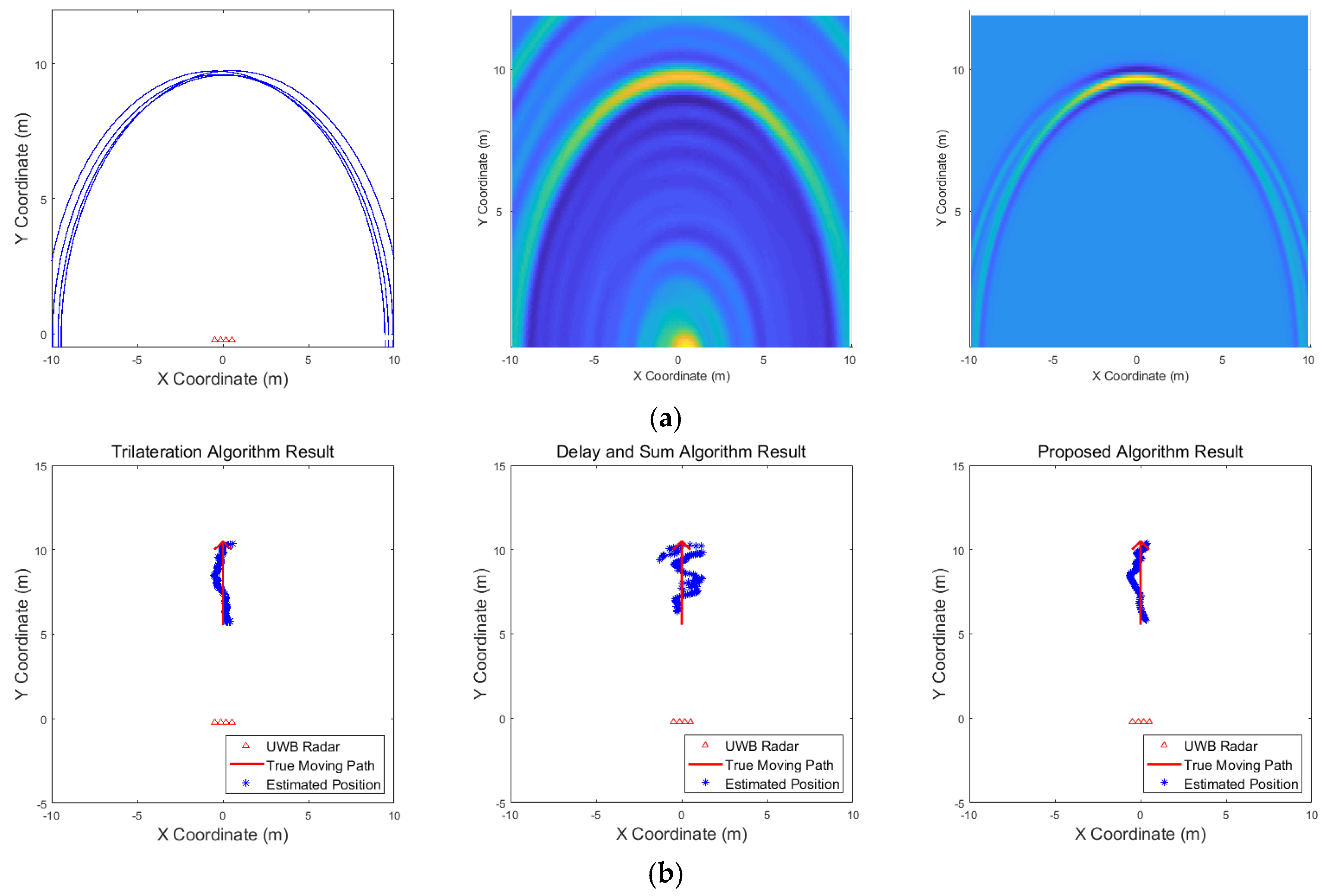
3.4. Performance Comparison by Simulation
4. Experimental Results Based on the Designed Through-wall Radar Hardware
5. Conclusions
Author Contributions
Acknowledgments
Conflicts of Interest
References
- Choi, J.W.; Quan, X.J.; Cho, S.H. Bi-directional passing people counting system based on IR-UWB radar sensors. IEEE Internet Things 2017, 5, 512–522. [Google Scholar] [CrossRef]
- Peabody, J.E.; Charvat, G.L.; Goodwin, J.; Tobias, M. Through-Wall Imaging Radar; Massachusetts Institute of Technology-Lincoln Laboratory: Lexington, KY, USA, 2012. [Google Scholar]
- Choi, J.W.; Yim, D.H.; Cho, S.H. People counting based on an IR-UWB radar sensor. IEEE Sens. J. 2017, 17, 5717–5727. [Google Scholar] [CrossRef]
- Gulmezoglu, B.; Guldogan, M.B.; Gezici, S. Multiperson tracking with a network of ultrawideband radar sensors based on Gaussian mixture PHD filters. IEEE Sens. J. 2014, 15, 2227–2237. [Google Scholar] [CrossRef]
- Bartoletti, S.; Giorgetti, A.; Win, M.Z.; Conti, A. Blind selection of representative observations for sensor radar networks. IEEE Trans. Veh. Technol. 2015, 64, 1388–1400. [Google Scholar] [CrossRef]
- Sobhani, B.; Paolini, E.; Giorgetti, A.; Mazzotti, M. Target tracking for UWB multistatic radar sensor networks. IEEE J. Sel. Top. Signal Process. 2013, 8, 125–136. [Google Scholar] [CrossRef]
- Chiani, M.; Giorgetti, A.; Mazzotti, M.; Minutolo, R.; Paolini, E. Target detection metrics and tracking for UWB radar sensor networks. In Proceedings of the 2009 IEEE International Conference on Ultra-Wideband, Vancouver, BC, Canada, 9–11 September 2009; pp. 469–474. [Google Scholar]
- Chiani, M.; Giorgetti, A.; Paolini, E. Sensor radar for object tracking. Proc. IEEE 2018, 106, 1022–1041. [Google Scholar] [CrossRef]
- Zhang, Z.; Zhang, X.; Lv, H.; Lu, G.H.; Jing, X.J.; Wang, J.Q. Human-target detection and surrounding structure estimation under a simulated rubble via UWB radar. IEEE Geosci. Remote Sens. Lett. 2012, 10, 328–331. [Google Scholar] [CrossRef]
- Li, J.; Zeng, Z.F.; Sun, J.G.; Liu, F.S. Through-wall detection of human being’s movement by UWB radar. IEEE Geosci. Remote Sens. Lett. 2012, 9, 1079–1083. [Google Scholar] [CrossRef]
- Yan, J.M.; Hong, H.; Zhao, H.; Li, Y.S.; Gu, C.; Zhu, X.H. Through-wall multiple targets vital signs tracking based on VMD algorithm. Sensors 2016, 16, 1293. [Google Scholar] [CrossRef]
- Ritchie, M.; Ash, M.; Chen, Q.C.; Chetty, K. Through wall radar classification of human micro-Doppler using singular value decomposition analysis. Sensors 2016, 16, 1401. [Google Scholar] [CrossRef]
- Liang, X.L.; Zhang, H.; Ye, S.B.; Fang, G.Y.; Gulliver, T.A. Improved denoising method for through-wall vital sign detection using UWB impulse radar. Digital Signal Process. 2018, 74, 72–93. [Google Scholar] [CrossRef]
- Liang, S.D. Sense-through-wall human detection based on UWB radar sensors. Signal Process. 2016, 126, 117–124. [Google Scholar] [CrossRef]
- Withington, P.; Fluhler, H.; Nag, S. Enhancing homeland security with advanced UWB sensors. IEEE Microwave Mag. 2003, 4, 51–58. [Google Scholar] [CrossRef]
- Nezirovic, A.; Yarovoy, A.G.; Ligthart, L.P. Signal processing for improved detection of trapped victims using UWB radar. IEEE Trans. Geosci. Remote Sens. 2009, 48, 2005–2014. [Google Scholar] [CrossRef]
- Sun, X.; Lu, B.Y.; Liu, P.F.; Zhou, Z.M. A multiarray refocusing approach for through-the-wall imaging. IEEE Geosci. Remote Sens. Lett. 2014, 12, 880–884. [Google Scholar] [CrossRef]
- Narayanan, R.M.; Gebhardt, E.T.; Broderick, S.P. Through-Wall Single and Multiple Target Imaging Using MIMO Radar. Electronics 2017, 6, 70. [Google Scholar] [CrossRef]
- Ma, Y.G.; Hong, H.; Zhu, X.H. Interaction multipath in through-the-wall radar imaging based on compressive sensing. Sensors 2018, 18, 549. [Google Scholar]
- Rovnakova, J.; Koucur, D. TOA estimation and data association for through-wall tracking of moving targets. Eurasip J. Wirel. Comm. 2010, 2010, 420767. [Google Scholar] [CrossRef]
- Chen, X.; Leung, H.; Tian, M. Multitarget detection and tracking for through-the-wall radars. IEEE Trans. Aerosp. Electron. Syst. 2014, 50, 1403–1415. [Google Scholar] [CrossRef]
- Stone, W.C. Electromagnetic Signal Attenuation in Construction Materials; 6055; National Institute of Standards and Technology: Gaithersburg, MD, USA, October 1997. [Google Scholar]
- Frazier, L.M. Radar surveillance through solid materials. SPIE 1997, 2938, 139–147. [Google Scholar]
- Aftanas, M.; Rovnakova, J.; Drutarovsky, M.; Kocur, D. Efficient method of TOA estimation for through wall imaging by UWB radar. In Proceedings of the 2008 IEEE International Conference on Ultra-Wideband, Hannover, Germany, 10–12 September 2008; pp. 101–104. [Google Scholar]
- Cassioli, D.; Win, M.Z.; Molisch, A.F. The ultra-wide bandwidth indoor channel: from statistical model to simulations. IEEE J. Sel. Areas Commun. 2002, 20, 1247–1257. [Google Scholar] [CrossRef]
- Mahafza, B.R. Radar Systems Analysis and Design Using MATLAB, 3rd ed.; CRC Press: Boca Raton, FL, USA, 2013. [Google Scholar]
- Rohling, H. Radar CFAR thresholding in clutter and multiple target situations. IEEE Trans. Aerosp. Electron. Syst. 1983, 4, 608–621. [Google Scholar] [CrossRef]
- Olyazadeh, R. Least Square Approach on Indoor Positioning Measurement Techniques. In Proceedings of the 2012 Conference on Geosciences, Geoinformation and Environment, Lisbon, Portugal, 9–10 November 2012. [Google Scholar]
- He, Y.; Xiu, J.J.; Guan, X. Radar Data Processing with Applications; John Wiley & Sons, Inc.: Singapore, 2016. [Google Scholar]
- Welch, G.; Bishop, G. An Introduction to the Kalman Filter; University of North Carolina at Chapel Hill: Chapel Hill, NC, USA, 1995. [Google Scholar]
- Park, J.S.; Baek, I.S.; Cho, S.H. Localizations of multiple targets using multistatic UWB radar systems. In Proceedings of the 2012 3rd IEEE International Conference on Network Infrastructure and Digital Content, Beijing, China, 21–23 September 2012; pp. 586–590. [Google Scholar]
- Chen, L.; Shan, O. A time-domain beamformer for UWB through-wall imaging. In Proceedings of the TENCON 2007–2007 IEEE Region 10 Conference, Taipei, Taiwan, 30 October–2 November 2007; pp. 1–4. [Google Scholar]
- Schachter, B.J. Automatic Target Recognition; SPIE Press: Bellingham, WA, USA, 2017. [Google Scholar]


| Parameter | Value |
|---|---|
| Central Frequency | 1.8 GHz |
| Bandwidth | 2.8 GHz |
| Average Transmission Power | −14 dBm |
| Parameter | Value |
|---|---|
| Position of Radar 1 | (−0.49, −0.22) (m) |
| Position of Radar 2 | (−0.14, −0.22) (m) |
| Position of Radar 3 | (0.16, −0.22) (m) |
| Position of Radar 4 | (0.51, −0.22) (m) |
| Detection rate of each radar | 75% |
| False alarm rate of each radar | 10% |
| Distance error of detected targets | Normal distribution with (m) |
| Index | Number of Targets | Scenario |
|---|---|---|
| Scenario 1 | 1 | One target standing at the coordinates (0, 6) (m) |
| Scenario 2 | 3 | Three targets standing at the coordinates (1, 4.5), (−1.5, 2.5) and (0, 8) (m) |
| Scenario 3 | 5 | Five targets standing at the coordinates (−4, 2), (−2, 6), (0, 9), (3, 7) and (4, 3) (m) |
| Scenario 4 | 2 | Two targets standing very close each other |
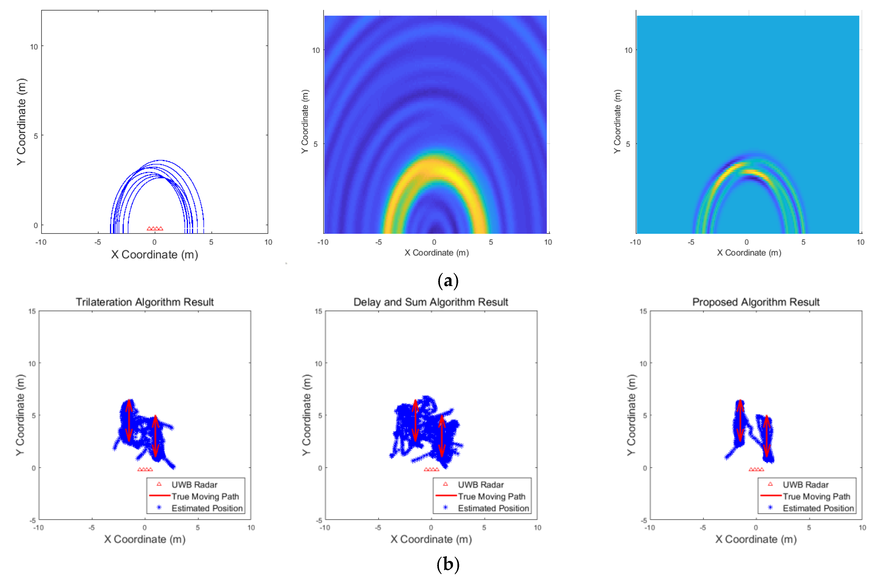
| Scenario 5 | 2 | Two targets moving cross along parallel paths |
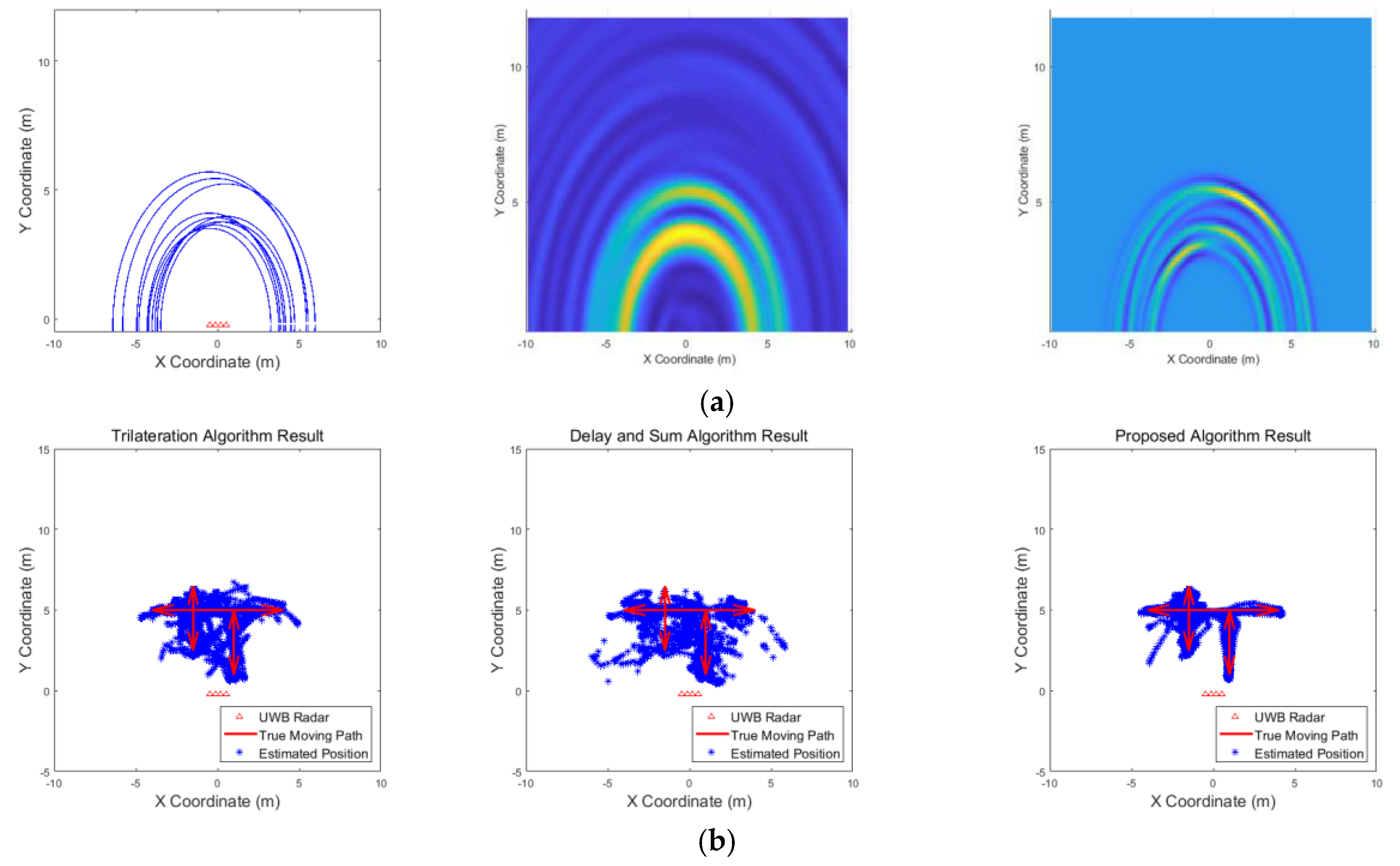
| Scenario 6 | 3 | Three targets moving along their respective paths |
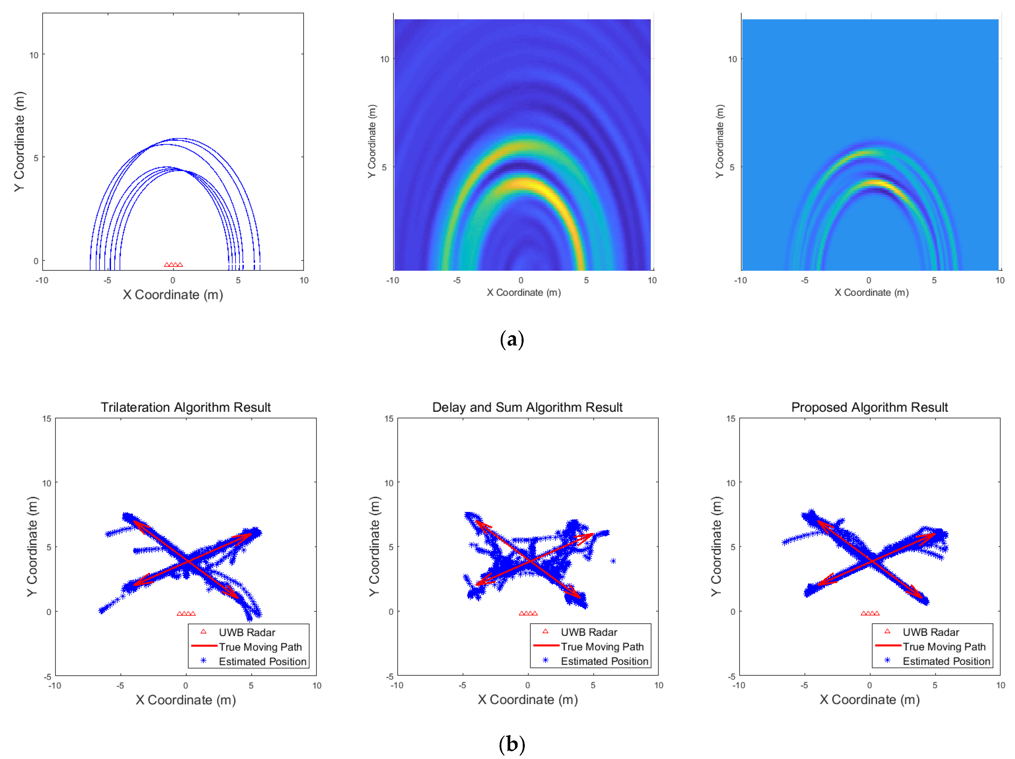
| Scenario 7 | 2 | Two targets moving cross over |
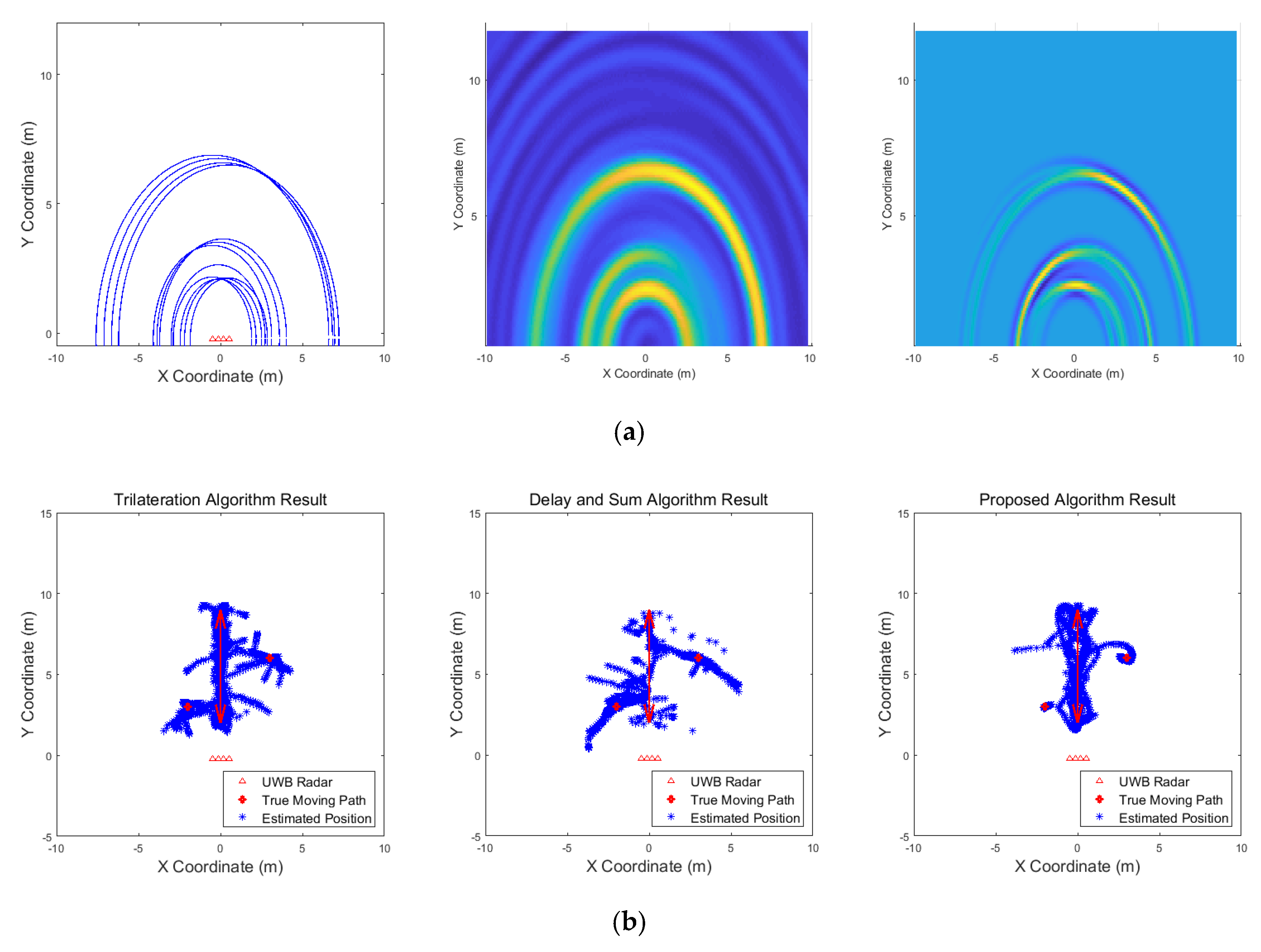
| Scenario 8 | 3 | Two targets standing and one target moving |
| Scenario 9 | 1 | One target moving in a circle |
| Scenario 10 | 2 | One target moving in a circle and one target moving horizontally |
| Scenario | Algorithm | Detection Rate (%) | False Alarm Rate (%) | |
|---|---|---|---|---|
| 1 | Trilateration | 100 | 2.43 | 0.05 |
| Delay and Sum | 99.86 | 33.95 | 1.22 | |
| Proposed Algorithm | 100 | 0.71 | 0.06 | |
| 2 | Trilateration | 99.76 | 3.99 | 0.20 |
| Delay and Sum | 98.95 | 44.37 | 2.13 | |
| Proposed Algorithm | 100 | 0 | 0.06 | |
| 3 | Trilateration | 75.29 | 0.86 | 0.93 |
| Delay and Sum | 94.41 | 57.49 | 7.02 | |
| Proposed Algorithm | 77.49 | 1.14 | 0.29 | |
| 4 | Trilateration | 98.93 | 21.26 | 0.86 |
| Delay and Sum | 54.99 | 0.57 | 6.08 | |
| Proposed Algorithm | 99.50 | 0 | 0.08 | |
| 5 | Trilateration | 98.29 | 2.14 | 0.47 |
| Delay and Sum | 93.15 | 25.11 | 1.24 | |
| Proposed Algorithm | 99.14 | 1.43 | 0.09 | |
| 6 | Trilateration | 90.35 | 7.56 | 0.59 |
| Delay and Sum | 78.22 | 8.70 | 1.00 | |
| Proposed Algorithm | 95.91 | 1.43 | 0.24 | |
| 7 | Trilateration | 92.15 | 0.71 | 0.42 |
| Delay and Sum | 80.39 | 8.27 | 1.05 | |
| Proposed Algorithm | 92.94 | 0.43 | 0.13 | |
| 8 | Trilateration | 99.52 | 12.27 | 0.68 |
| Delay and Sum | 79.89 | 8.56 | 1.22 | |
| Proposed Algorithm | 98.48 | 1.71 | 0.13 | |
| 9 | Trilateration | 99.29 | 1.14 | 0.14 |
| Delay and Sum | 98.43 | 12.13 | 0.59 | |
| Proposed Algorithm | 100 | 0.29 | 0.13 | |
| 10 | Trilateration | 96.36 | 1.43 | 0.29 |
| Delay and Sum | 93.22 | 25.82 | 1.62 | |
| Proposed Algorithm | 96.93 | 1.14 | 0.11 |
| Index | Scenario |
|---|---|
| Scenario 1 | One person standing with a natural position at the coordinates (0, 6) (m) |
| Scenario 2 | Three persons standing with a natural position at (−1, 4), (2, 6) and (0, 9) (m) |
| Scenario 3 | One person walking back and forth in the radar coverage area |
| Scenario | Algorithm | Detection Rate (%) | False Alarm Rate (%) | |
|---|---|---|---|---|
| 1 | Trilateration | 100 | 0 | 0.03 |
| Delay and Sum | 100 | 2.18 | 0.57 | |
| Proposed Algorithm | 100 | 0 | 0.09 | |
| 2 | Trilateration | 84.53 | 1.63 | 1.35 |
| Delay and Sum | 79.17 | 5.90 | 2.35 | |
| Proposed Algorithm | 86.65 | 0.64 | 0.89 | |
| 3 | Trilateration | 100 | 0 | 0.12 |
| Delay and Sum | 97.59 | 14.82 | 0.49 | |
| Proposed Algorithm | 100 | 0 | 0.19 |
© 2019 by the authors. Licensee MDPI, Basel, Switzerland. This article is an open access article distributed under the terms and conditions of the Creative Commons Attribution (CC BY) license (http://creativecommons.org/licenses/by/4.0/).
Share and Cite
Yoo, S.; Wang, D.; Seol, D.-M.; Lee, C.; Chung, S.; Cho, S.H. A Multiple Target Positioning and Tracking System Behind Brick-Concrete Walls Using Multiple Monostatic IR-UWB Radars. Sensors 2019, 19, 4033. https://0-doi-org.brum.beds.ac.uk/10.3390/s19184033
Yoo S, Wang D, Seol D-M, Lee C, Chung S, Cho SH. A Multiple Target Positioning and Tracking System Behind Brick-Concrete Walls Using Multiple Monostatic IR-UWB Radars. Sensors. 2019; 19(18):4033. https://0-doi-org.brum.beds.ac.uk/10.3390/s19184033
Chicago/Turabian StyleYoo, Sungwon, Dingyang Wang, Dong-Min Seol, Chulsoo Lee, Sungmoon Chung, and Sung Ho Cho. 2019. "A Multiple Target Positioning and Tracking System Behind Brick-Concrete Walls Using Multiple Monostatic IR-UWB Radars" Sensors 19, no. 18: 4033. https://0-doi-org.brum.beds.ac.uk/10.3390/s19184033