An Improved Imaging Algorithm for High-Resolution Spotlight SAR with Continuous PRI Variation Based on Modified Sinc Interpolation


Abstract
:1. Introduction
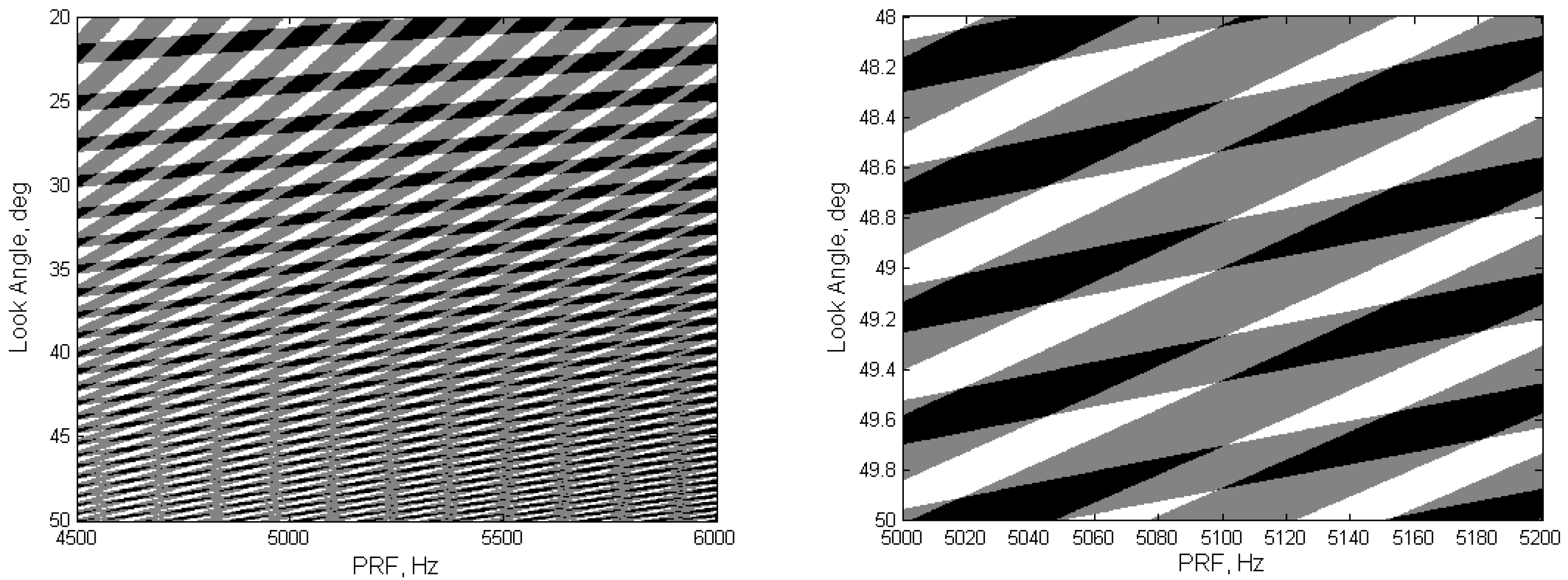
2. PRI Variation
2.1. Fixed PRI
2.2. Periodically Varied PRI
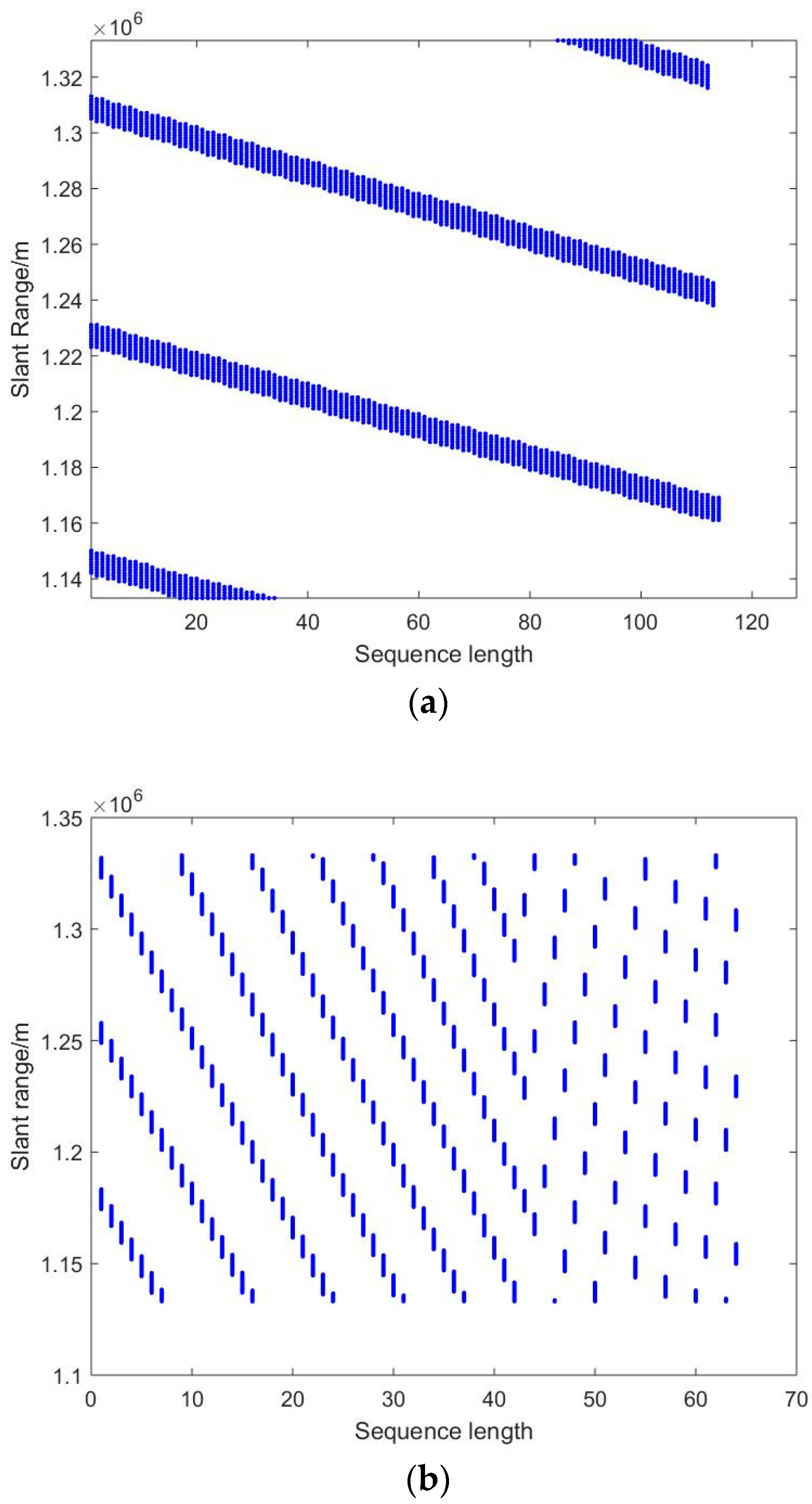
2.2.1. Slow Linear Variation
2.2.2. Fast Linear Variation
2.2.3. SAR Parameters of Two Types of PRI Variations
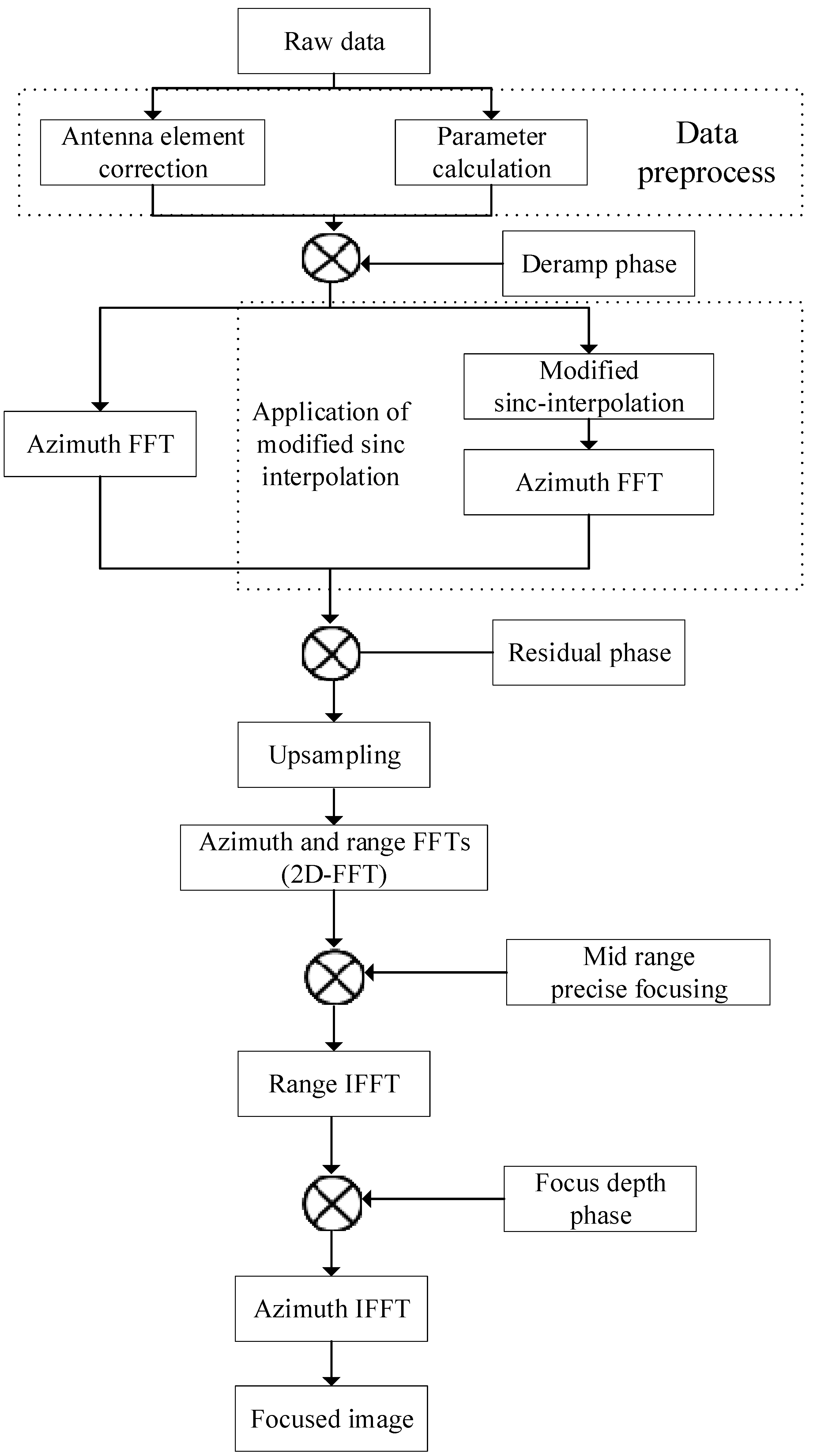
3. Imaging Algorithm for Spotlight SAR with PRI Variation
3.1. Modified Sinc Interpolation
3.2. Modified Two-Step Processing Approach Based on Modified Sinc Interpolation
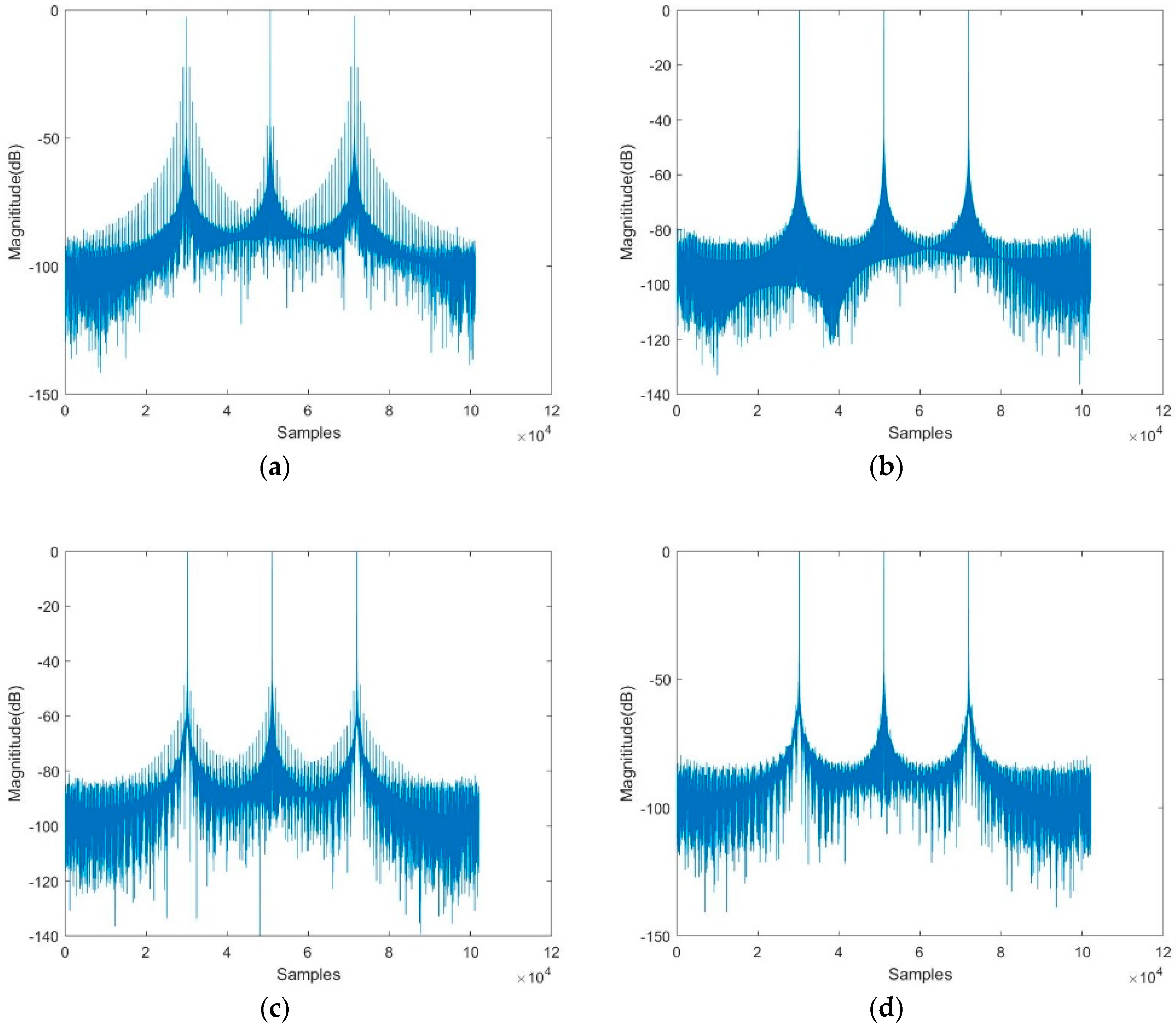
4. Simulation Results
4.1. Results of Slow PRI Variation
4.2. Results of Fast PRI Variation
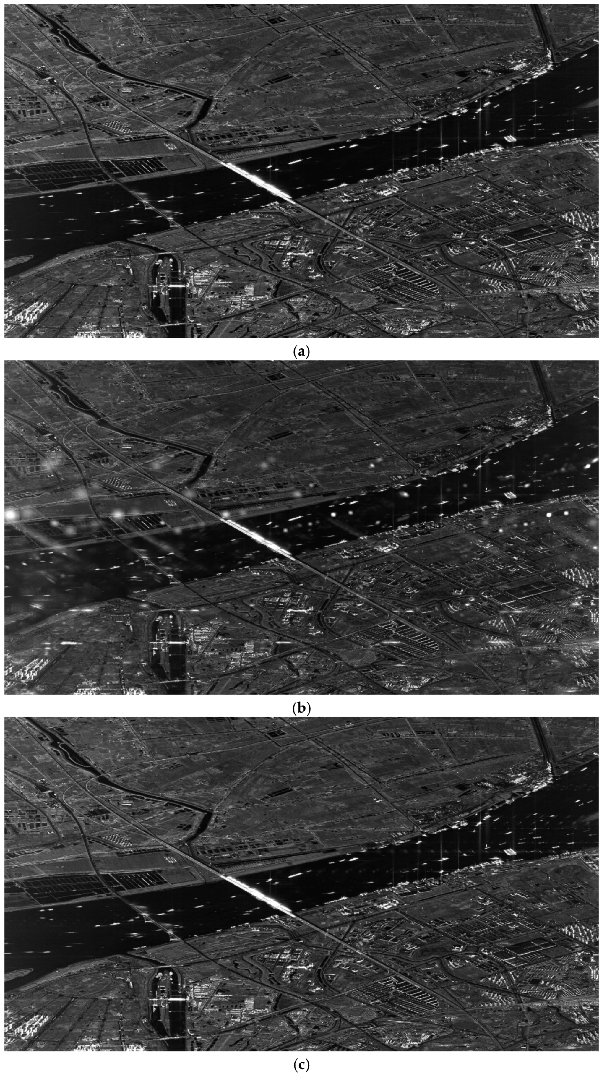
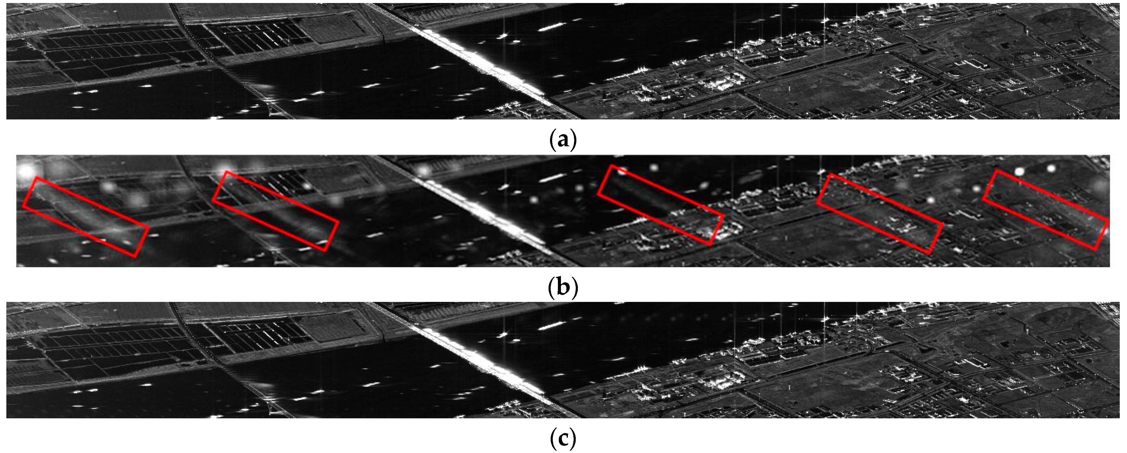
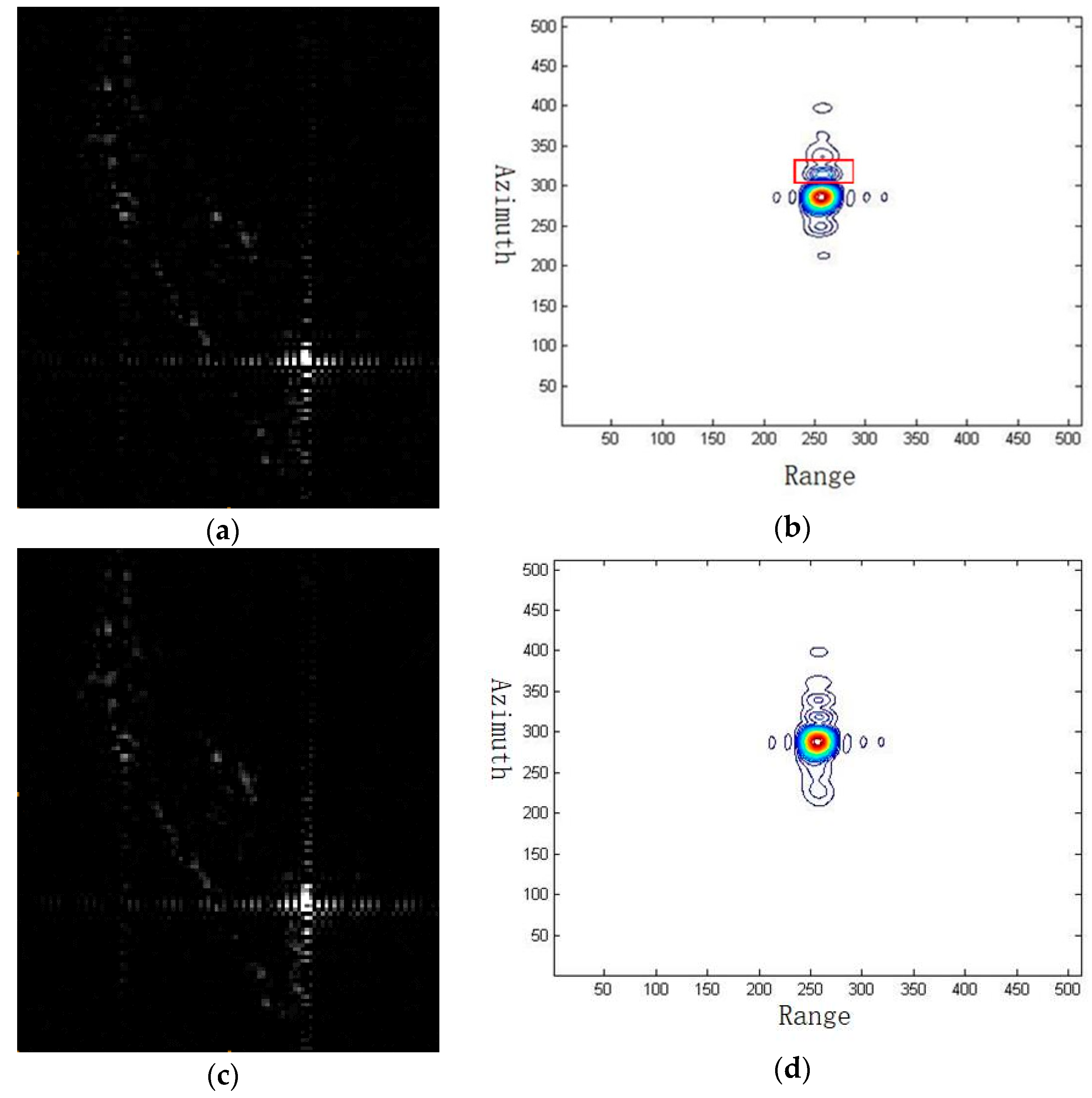
4.3. Experiments on GF-3 Data
5. Conclusions
Author Contributions
Funding
Acknowledgments
Conflicts of Interest
References
- Currie, A.; Brown, M.A. Wide-swath SAR. IEE Proc. F-Radar Signal Process 1992, 139, 122–135. [Google Scholar] [CrossRef]
- Krieger, G.; Gebert, N.; Younis, M.; Moreira, A. Advanced synthetic aperture radar based on digital beamforming and waveform diversity. In Proceedings of the 2008 IEEE Radar Conference, Rome, Italy, 26–30 May 2008. [Google Scholar]
- Imaging, H.W.; Xu, W.; Deng, Y. Multichannel SAR with Reflector Antenna. IEEE Antennas Wirel. Propag. Lett. 2010, 9, 1123–1126. [Google Scholar]
- Wang, W.A. Space—Time Coding MIMO-OFDM SAR for High-Resolution Imaging. IEEE Trans. Geosci. Remote Sens. 2011, 49, 3094–3104. [Google Scholar] [CrossRef]
- Krieger, G.; Gebert, N.; Moreira, A. SAR signal reconstruction from non-uniform displaced phase centre sampling. In Proceedings of the IEEE International Geoscience and Remote Sensing Symposium (IGARSS 2004), Anchorage, AK, USA, 20–24 September 2004; Volume 3, pp. 1763–1766. [Google Scholar]
- Zhao, S.; Wang, R.; Deng, Y.; Zhang, Z.; Li, N.; Guo, L.; Wang, W. Modifications on Multichannel Reconstruction Algorithm for SAR Processing Based on Periodic Nonuniform Sampling Theory and Nonuniform Fast Fourier Transform. IEEE J. Sel. Top. Appl. Earth Obs. Remote Sens. 2015, 8, 4998–5006. [Google Scholar] [CrossRef]
- Subiza, B.; Gimeno-Nieves, E.; Lopez-Sanchez, J.M.; Fortuny-Guasch, J. An approach to SAR imaging by means of non-uniform FFTs. In Proceedings of the IEEE International Geoscience and Remote Sensing Symposium (IGARSS 2003, IEEE Cat. No.03CH37477), Toulous, France, 21–25 July 2003; Volume 6, pp. 4089–4091. [Google Scholar]
- Villano, M.; Jäger, M.; Steinbrecher, U. Staggered SAR: Imaging a Wide Continuous Swath by Continuous PRI Variation. Kleinheubacher Tag. 2014, 52, 4462–4479. [Google Scholar]
- Ding, Y.; Munson, D.C.J. A fast back-projection algorithm for bistatic SAR imaging. In Proceedings of the International Conference on Image Processing, Rochester, NY, USA, 22–25 September 2002. [Google Scholar]
- Zhang, L.; Li, H.; Qiao, Z.; Xu, Z. A Fast BP Algorithm with Wavenumber Spectrum Fusion for High-Resolution Spotlight SAR Imaging. IEEE Geosci. Remote Sens. Lett. 2014, 11, 1460–1464. [Google Scholar] [CrossRef]
- Villano, M.; Krieger, G.; Moreira, A. Staggered-SAR for high-resolution wide-swath imaging. In Proceedings of the IET International Conference on Radar Systems (Radar 2012), Glasgow, UK, 22–25 October 2012. [Google Scholar]
- Luo, X.; Wang, R.; Xu, W.; Deng, Y.; Guo, L. Modification of multichannel reconstruction algorithm on the SAR with linear variation of PRI. IEEE J. Sel. Top. Appl. Earth Obs. Remote Sens. 2014, 7, 3050–3059. [Google Scholar] [CrossRef]
- Dutt, A.; Rokhlin, V. Fast Fourier Transforms for Nonequispaced Data. Siam J. Sci. Comput. 1993, 14, 1368–1393. [Google Scholar] [CrossRef] [Green Version]
- Maymon, S.; Oppenheim, A.V. Sinc interpolation of nonuniform samples. IEEE Trans. Signal Process. 2011, 59, 4745–4758. [Google Scholar] [CrossRef]
- Hanssen, R.; Bamler, R. Evaluation of interpolation kernels for SAR interferometry. IEEE Trans. Geosci. Remote Sens. 1999, 37, 318–321. [Google Scholar] [CrossRef]
- Li, Z.; Bethel, J. Image coregistration in SAR interferometry. Int. Arch. Photogramm. Remote Sens. Spat. Inf. Sci. 2008, 37, 433–438. [Google Scholar]
- Lanari, R.; Tesauro, M.; Sansosti, E.; Fornaro, G. Spotlight SAR data focusing based on a two-step processing approach. IEEE Trans. Geosci. Remote Sens. 2001, 39, 1993–2004. [Google Scholar] [CrossRef]
- Lanari, R.; Zoffoli, S.; Sansosti, E.; Fornaro, G.; Serafino, F. New approach for hybrid strip-map/spotlight SAR data focusing. IEE Proc. Radar Sonar Navig. 2001, 148, 363. [Google Scholar] [CrossRef]
- Mittermayer, J.; Moreira, A.; Loffeld, O. Spotlight SAR data processing using the frequency scaling algorithm. IEEE Trans. Geosci. Remote Sens. 1999, 37, 2198–2214. [Google Scholar] [CrossRef]
- Eineder, M.; Adam, N.; Bamler, R.; Yague-Martinez, N.; Breit, H. Spaceborne spotlight SAR interferometry with TerraSAR-X. IEEE Trans. Geosci. Remote Sens. 2009, 47, 1524–1535. [Google Scholar] [CrossRef]


| Parameter | Value |
|---|---|
| Wavelength (m) | 0.0312 |
| Orbit height (km) | 1100 |
| Look angle (degree) | 49 |
| PRF span (Slow change) (Hz) | 3243–3355 |
| PRF span (Fast change) (Hz) | 3243–5964 |
| Pulse duration (µs) | 30 |
| Pulse number in a sequence period (Slow change) | 110 |
| Pulse number in a sequence period (Fast change) | 64 |
| Nominal azimuth Resolution | 0.1 |
| Illuminated area (km) | 8 |
| Methods | Complex Multipication | Complex Additons | Total |
|---|---|---|---|
| NUDFT | Na2 | Na × (Na − 1) | Na × (2Na − 1) |
| Modified sinc interpolation | Na × L | Na × (L − 1) | Na × (2L − 1) |
| Variation of PRI | Algorithm | Near-Range Target | Mid-Range Target | Far-Range Target |
|---|---|---|---|---|
| Slow linear variation of PRI | FFT | −20.56 dB | −48.44 dB | −22.11 dB |
| NUDFT | −71.56 dB | −72.91 dB | −72.57 dB | |
| Traditional sinc | −49.38 dB | −50.17 dB | −49.87 dB | |
| Modified sinc | −67.22 dB | −66.89 dB | −71.61 dB | |
| Fast linear variation of PRI | FFT | −12.33 dB | −31.98 dB | −12.04 dB |
| NUDFT | −54.03 dB | −54.25 dB | −54.57 dB | |
| Traditional sinc | −26.05 dB | −26.11 dB | −26.02 dB | |
| Modified sinc | −56.48 dB | −53.36 dB | −54.95 dB |
| Method | PSLR | ISLR |
|---|---|---|
| Conventional two-step processing approach | −10.954 dB | −10.067 dB |
| Modified two-step processing approach | −13.844 dB | −12.130 dB |
© 2019 by the authors. Licensee MDPI, Basel, Switzerland. This article is an open access article distributed under the terms and conditions of the Creative Commons Attribution (CC BY) license (http://creativecommons.org/licenses/by/4.0/).
Share and Cite
Chen, S.; Huang, L.; Qiu, X.; Shang, M.; Han, B. An Improved Imaging Algorithm for High-Resolution Spotlight SAR with Continuous PRI Variation Based on Modified Sinc Interpolation. Sensors 2019, 19, 389. https://0-doi-org.brum.beds.ac.uk/10.3390/s19020389
Chen S, Huang L, Qiu X, Shang M, Han B. An Improved Imaging Algorithm for High-Resolution Spotlight SAR with Continuous PRI Variation Based on Modified Sinc Interpolation. Sensors. 2019; 19(2):389. https://0-doi-org.brum.beds.ac.uk/10.3390/s19020389
Chicago/Turabian StyleChen, Shiyang, Lijia Huang, Xiaolan Qiu, Mingyang Shang, and Bing Han. 2019. "An Improved Imaging Algorithm for High-Resolution Spotlight SAR with Continuous PRI Variation Based on Modified Sinc Interpolation" Sensors 19, no. 2: 389. https://0-doi-org.brum.beds.ac.uk/10.3390/s19020389