Automatic Change Detection System over Unmanned Aerial Vehicle Video Sequences Based on Convolutional Neural Networks

 , , , ,
Abstract
:1. Introduction
2. Related Work
2.1. Change Detection Using Traditional Image Processing
2.2. Convolutional Neural Networks
- Convolutional layers perform a dot product between each region of the input and a filter. These filters, also known as kernels, define the size of the mentioned regions. With this operation, the layer is capable of obtaining the most significant features of the input. The number of filters typically varies from each convolutional layer, in order to obtain higher or lower level features. The resultant structure depends on the padding employed on the convolution.
- Activation layers execute a predefined function to their inputs. The aim of these layers is to characterize the features obtained from the previous layers to obtain the most relevant ones. This process is performed using diverse functions, which may vary among the systems.
- Pooling layers down-sample their input, obtaining the most significant values from each region. Most CNNs employ a 2 × 2 kernel in their pooling layers. With this region size, the input is down-sampled by half in both dimensions, width and height.
2.3. CNN-Based Change Detection
2.4. Image Matching Techniques
3. Methodology
3.1. Image Alignment
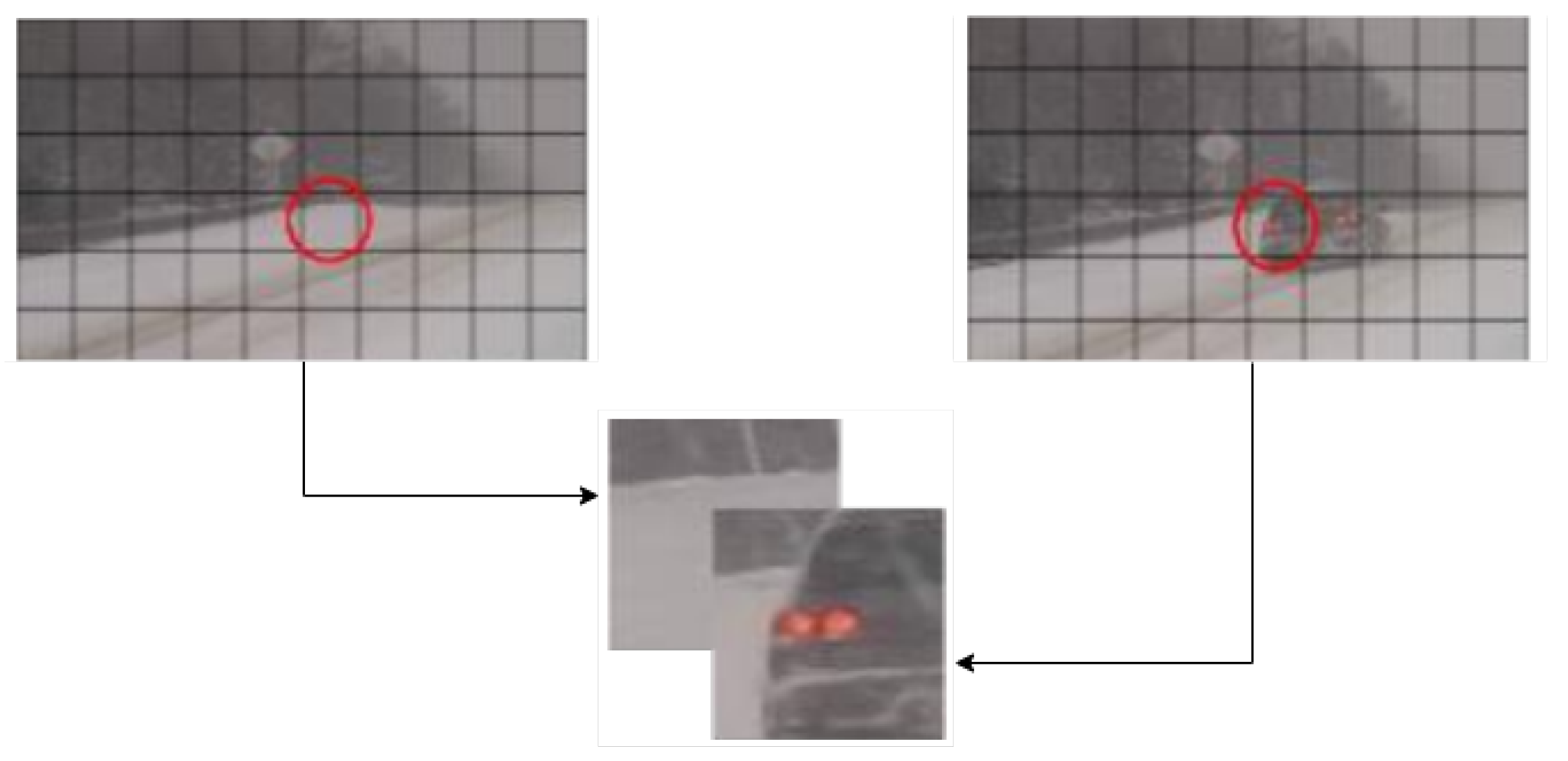
3.2. Sliding Window
3.3. Deep Neural Network Architecture
3.4. Dataset
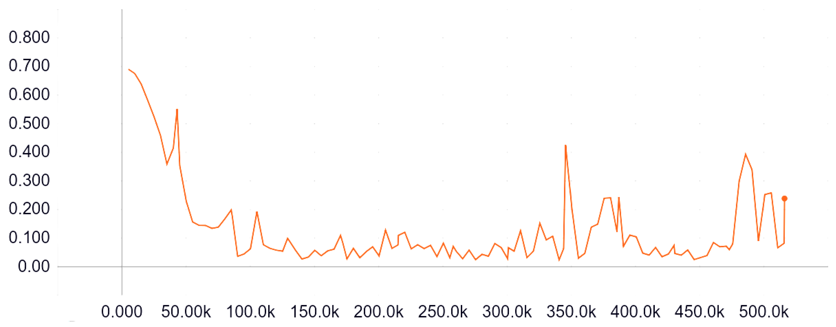
3.5. Training
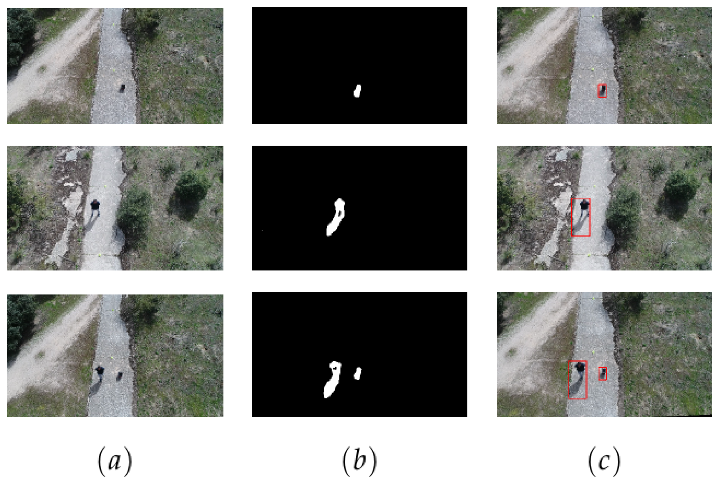
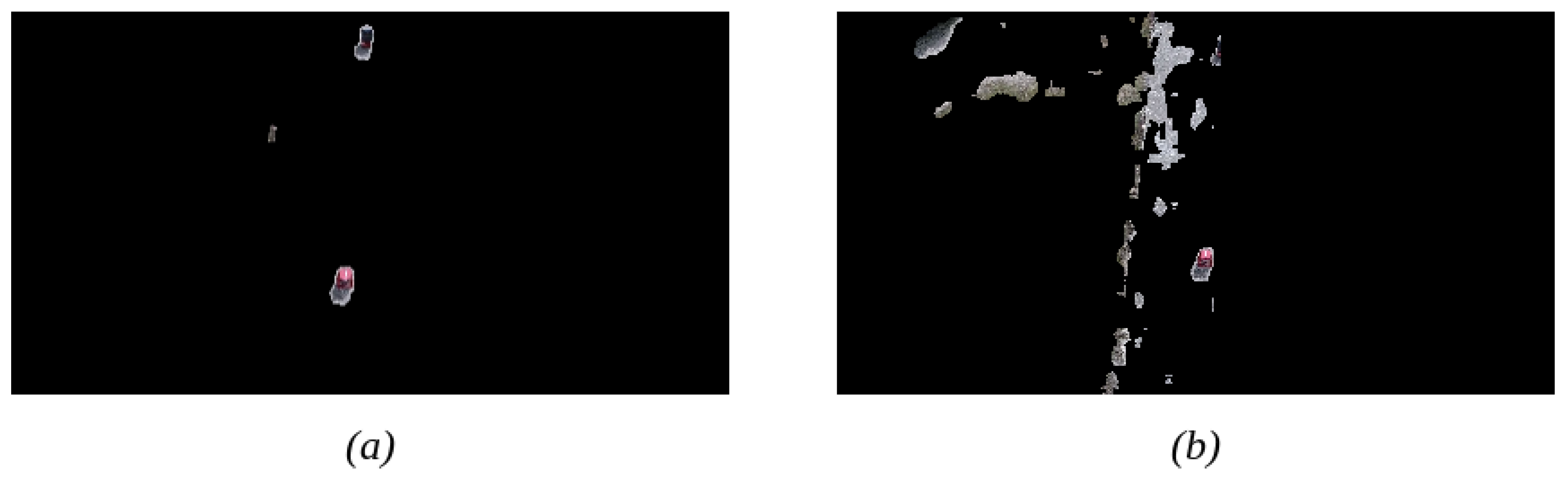
3.6. Post Processing
4. Experimental Results
4.1. Evaluation Metrics
- Recall (Re):
- Specificity (Sp):
- False Positive Rate (FPR):
- False Negative Rate (FNR):
- Percentage of Wrong Classifications (PWC):
- Precision (Pr):
- F-measure (FM):
4.2. Comparison with Other Change Detection Systems
5. Discussion
6. Conclusions
Future Work
Author Contributions
Funding
Conflicts of Interest
References
- Wang, Y.; Jodoin, P.; Porikli, F.; Konrad, J.; Benezeth, Y.; Ishwar, P. CDnet 2014: An Expanded Change Detection Benchmark Dataset. In Proceedings of the 2014 IEEE Conference on Computer Vision and Pattern Recognition Workshops, Columbus, OH, USA, 23–28 June 2014; pp. 393–400. [Google Scholar] [CrossRef]
- Minematsu, T.; Shimada, A.; Uchiyama, H.; Charvillat, V.; Taniguchi, R.I. Reconstruction-Base Change Detection with Image Completion for a Free-Moving Camera. Sensors 2018, 18, 1232. [Google Scholar] [CrossRef] [PubMed]
- Babaee, M.; Dinh, D.T.; Rigoll, G. A Deep Convolutional Neural Network for Video Sequence Background Subtraction. Pattern Recogn. 2018, 76, 635–649. [Google Scholar] [CrossRef]
- Braham, M.; Van Droogenbroeck, M. Deep background subtraction with scene-specific convolutional neural networks. In Proceedings of the 2016 International Conference on Systems, Signals and Image Processing (IWSSIP), Bratislava, Slovakia, 23–25 May 2016; pp. 1–4. [Google Scholar]
- St-Charles, P.; Bilodeau, G.; Bergevin, R. Universal Background Subtraction Using Word Consensus Models. IEEE Trans. Image Process. 2016, 25, 4768–4781. [Google Scholar] [CrossRef]
- Stauffer, C.; Grimson, W.E.L. Adaptive background mixture models for real-time tracking. In Proceedings of the 1999 IEEE Computer Society Conference on Computer Vision and Pattern Recognition (Cat. No PR00149), Fort Collins, CO, USA, 23–25 June 1999; Volume 2, pp. 246–252. [Google Scholar] [CrossRef]
- Elgammal, A.M.; Harwood, D.; Davis, L.S. Non-parametric Model for Background Subtraction. In Proceedings of the 6th European Conference on Computer Vision-Part II, Dublin, Ireland, 26 June–1 July 2000; Springer: London, UK, 2000; pp. 751–767. [Google Scholar]
- St-Charles, P.; Bilodeau, G.; Bergevin, R. SuBSENSE: A Universal Change Detection Method With Local Adaptive Sensitivity. IEEE Trans. Image Process. 2015, 24, 359–373. [Google Scholar] [CrossRef] [PubMed]
- Barnich, O.; Van Droogenbroeck, M. ViBe: A Universal Background Subtraction Algorithm for Video Sequences. IEEE Trans. Image Process. 2011, 20, 1709–1724. [Google Scholar] [CrossRef] [PubMed]
- LeCun, Y.; Haffner, P.; Bottou, L.; Bengio, Y. Object Recognition with Gradient-Based Learning. In Shape, Contour and Grouping in Computer Vision; Springer: London, UK, 1999; pp. 319–345. [Google Scholar]
- Szegedy, C.; Liu, W.; Jia, Y.; Sermanet, P.; Reed, S.E.; Anguelov, D.; Erhan, D.; Vanhoucke, V.; Rabinovich, A. Going Deeper with Convolutions. In Proceedings of the 2015 IEEE Conference on Computer Vision and Pattern Recognition (CVPR), Boston, MA, USA, 7–12 June 2014. [Google Scholar]
- Zeng, D.; Zhu, M. Background Subtraction Using Multiscale Fully Convolutional Network. IEEE Access 2018, 6, 16010–16021. [Google Scholar] [CrossRef]
- Liu, S.; Deng, W. Very deep convolutional neural network based image classification using small training sample size. In Proceedings of the 2015 3rd IAPR Asian Conference on Pattern Recognition (ACPR), Kuala Lumpur, Malaysia, 3–6 November 2015; pp. 730–734. [Google Scholar] [CrossRef]
- Coombes, M.; McAree, O.; Chen, W.; Render, P. Development of an autopilot system for rapid prototyping of high level control algorithms. In Proceedings of the 2012 UKACC International Conference on Control, Cardiff, UK, 3–5 September 2012; pp. 292–297. [Google Scholar] [CrossRef]
- Rublee, E.; Rabaud, V.; Konolige, K.; Bradski, G. ORB: An efficient alternative to SIFT or SURF. In Proceedings of the 2011 International Conference on Computer Vision, Barcelona, Spain, 6–13 November 2011; pp. 2564–2571. [Google Scholar] [CrossRef]
- Calonder, M.; Lepetit, V.; Strecha, C.; Fua, P. Brief: Binary robust independent elementary features. In Proceedings of the European Conference on Computer Vision, Crete, Greece, 5–11 September 2010; Springer: Berlin, Germany, 2010; pp. 778–792. [Google Scholar]
- Rosten, E.; Drummond, T. Machine learning for high-speed corner detection. In Proceedings of the European Conference on Computer Vision, Graz, Austria, 7–13 May 2006; Springer: Berlin, Germany; pp. 430–443. [Google Scholar]
- Harris, C.; Stephens, M. A Combined Corner and Edge Detector. In Proceedings of the 4th Alvey Vision Conference, Manchester, UK, 31 August–2 September 1988; pp. 147–151. [Google Scholar]
- Rosin, P.L. Measuring Corner Properties. Comput. Vis. Image Underst. 1999, 73, 291–307. [Google Scholar] [CrossRef] [Green Version]
- Lowe, D.G. Distinctive Image Features from Scale-Invariant Keypoints. Int. J. Comput. Vision 2004, 60, 91–110. [Google Scholar] [CrossRef]
- Bay, H.; Ess, A.; Tuytelaars, T.; Van Gool, L. Speeded-up robust features (SURF). Comput. Vis. Image Underst. 2008, 110, 346–359. [Google Scholar] [CrossRef]
- Avola, D.; Cinque, L.; Foresti, G.L.; Martinel, N.; Pannone, D.; Piciarelli, C. A UAV Video Dataset for Mosaicking and Change Detection From Low-Altitude Flights. IEEE Trans. Syst. Man, Cybern. Syst. 2018, 1–11. [Google Scholar] [CrossRef]
- Laganiere, R. OpenCV Computer Vision Application Programming Cookbook Second Edition; Packt Publishing Ltd.: Birmingham, UK, 2014. [Google Scholar]
- Hahnloser, R.; Sarpeshkar, R.; Mahowald, M.A.; Douglas, R.; Sebastian Seung, H. Digital selection and analogue amplification coexist in a cortex-inspired silicon circuit. Nature 2000, 405, 947–951. [Google Scholar] [CrossRef] [PubMed]
- Srivastava, N.; Hinton, G.; Krizhevsky, A.; Sutskever, I.; Salakhutdinov, R. Dropout: A Simple Way to Prevent Neural Networks from Overfitting. J. Mach. Learn. Res. 2014, 15, 1929–1958. [Google Scholar]
- Caruana, R.; Lawrence, S.; Giles, L. Overfitting in Neural Nets: Backpropagation, Conjugate Gradient, and Early Stopping. In Proceedings of the 13th International Conference on Neural Information Processing Systems, Hong Kong, China, 3–6 October 2000; MIT Press: Cambridge, MA, USA, 2000; pp. 381–387. [Google Scholar]
- Ioffe, S.; Szegedy, C. Batch Normalization: Accelerating Deep Network Training by Reducing Internal Covariate Shift. In Proceedings of the 32Nd International Conference on International Conference on Machine Learning, Lille, France, 6–11 July 2015; Volume 37, pp. 448–456. [Google Scholar]
- Keras: Deep Learning for Humans. Available online: https://github.com/fchollet/keras (accessed on 27 November 2018).
- Abadi, M.; Barham, P.; Chen, J.; Chen, Z.; Davis, A.; Dean, J.; Devin, M.; Ghemawat, S.; Irving, G.; Isard, M.; et al. TensorFlow: A System for Large-scale Machine Learning. In Proceedings of the 12th USENIX Conference on Operating Systems Design and Implementation, Savannah, GA, USA, 2–4 November 2016; USENIX Association: Berkeley, CA, USA, 2016; pp. 265–283. [Google Scholar]
- van der Walt, S.; Colbert, S.C.; Varoquaux, G. The NumPy Array: A Structure for Efficient Numerical Computation. Comput. Sci. Eng. 2011, 13, 22–30. [Google Scholar] [CrossRef] [Green Version]
- Prechelt, L. Early stopping-but when? In Neural Networks: Tricks of the Trade; Springer: Berlin, Germany, 1998; pp. 55–69. [Google Scholar]
- Hofmann, M.; Tiefenbacher, P.; Rigoll, G. Background segmentation with feedback: The pixel-based adaptive segmenter. In Proceedings of the 2012 IEEE Computer Society Conference on Computer Vision and Pattern Recognition Workshops, Providence, RI, USA, 16–21 June 2012; pp. 38–43. [Google Scholar]


| Name | Input Size | Kernel | Stride | Output Size |
|---|---|---|---|---|
| conv2d1 | 64 × 64 × 6 | 3 × 3 | 1 | 64 × 64 × 24 |
| pool1 | 64 × 64 × 24 | - | 2 | 32 × 32 × 24 |
| conv2d2 | 32 × 32 × 24 | 3 × 3 | 1 | 32 × 32 × 48 |
| pool2 | 32 × 32 × 48 | - | 2 | 16 × 16 × 48 |
| conv2d3 | 16 × 16 × 48 | 3 × 3 | 1 | 16 × 16 × 96 |
| pool3 | 16 × 16 × 96 | - | 2 | 8 × 8 × 96 |
| conv2d4 | 8 × 8 × 96 | 3 × 3 | 1 | 8 × 8 × 96 |
| pool4 | 8 × 8 × 96 | - | 2 | 4 × 4 × 96 |
| Name | Input Size | Function | Output Size |
|---|---|---|---|
| flatten | 4 × 4 × 96 | - | 1536 |
| bn | 1536 | Batch Normalization | 1536 |
| dp | 1536 | Dropout | 1536 |
| final | 1536 | Sigmoid | 4096 |
| Category | Images | Size | Total Patches |
|---|---|---|---|
| Blizzard (BW) | 195 | 1216 × 704 | 40,755 |
| Skating (BW) | 177 | 1216 × 704 | 36,993 |
| Snowfall (BW) | 192 | 1216 × 704 | 40,128 |
| Canoe (DBG) | 210 | 640 × 384 | 12,600 |
| Sofa (IOM) 1 | 150 | 320 × 192 | 6750 |
| Category | Sp | FPR | FNR | PWC | FM |
|---|---|---|---|---|---|
| Bad Weather (BW) | 0.999914 | 0.000086 | 0.022035 | 0.017216 | 0.977963 |
| Dynamic Background (DBG) | 0.999810 | 0.000190 | 0.048662 | 0.038013 | 0.951339 |
| Intermittent Object Motion (IOM) | 0.999790 | 0.000210 | 0.005232 | 0.004808 | 0.994768 |
| Implementation | FMoverall | FMBW | FMDBG | FMIOM |
|---|---|---|---|---|
| Proposed | 0.9747 | 0.9779 | 0.9513 | 0.9947 |
| ConvNet-GT [4] | 0.9054 | 0.9264 | 0.8845 | Unknown |
| ConvNet-IUTIS [4] | 0.8386 | 0.8849 | 0.7923 | Unknown |
| CNN [3] | 0.7718 | 0.8301 | 0.8761 | 0.6098 |
| GMM [6] | 0.6306 | 0.7380 | 0.6330 | 0.5207 |
| SuBSENSE [8] | 0,7788 | 0.8619 | 0.8177 | 0.6569 |
| PBAS [32] | 0.6749 | 0.7673 | 0.6829 | 0.5745 |
| PAWCS [5] | 0.8285 | 0.8152 | 0.8938 | 0.7764 |
© 2019 by the authors. Licensee MDPI, Basel, Switzerland. This article is an open access article distributed under the terms and conditions of the Creative Commons Attribution (CC BY) license (http://creativecommons.org/licenses/by/4.0/).
Share and Cite
García Rubio, V.; Rodrigo Ferrán, J.A.; Menéndez García, J.M.; Sánchez Almodóvar, N.; Lalueza Mayordomo, J.M.; Álvarez, F. Automatic Change Detection System over Unmanned Aerial Vehicle Video Sequences Based on Convolutional Neural Networks. Sensors 2019, 19, 4484. https://0-doi-org.brum.beds.ac.uk/10.3390/s19204484
García Rubio V, Rodrigo Ferrán JA, Menéndez García JM, Sánchez Almodóvar N, Lalueza Mayordomo JM, Álvarez F. Automatic Change Detection System over Unmanned Aerial Vehicle Video Sequences Based on Convolutional Neural Networks. Sensors. 2019; 19(20):4484. https://0-doi-org.brum.beds.ac.uk/10.3390/s19204484
Chicago/Turabian StyleGarcía Rubio, Víctor, Juan Antonio Rodrigo Ferrán, Jose Manuel Menéndez García, Nuria Sánchez Almodóvar, José María Lalueza Mayordomo, and Federico Álvarez. 2019. "Automatic Change Detection System over Unmanned Aerial Vehicle Video Sequences Based on Convolutional Neural Networks" Sensors 19, no. 20: 4484. https://0-doi-org.brum.beds.ac.uk/10.3390/s19204484