Comparison of Cooled and Uncooled IR Sensors by Means of Signal-to-Noise Ratio for NDT Diagnostics of Aerospace Grade Composites

 ,
,  , , , and
Abstract
:1. Introduction
2. Thermal Technology
2.1. Infrared Imaging Systems
2.2. Radiometry
2.3. Cooled and Uncooled Cameras
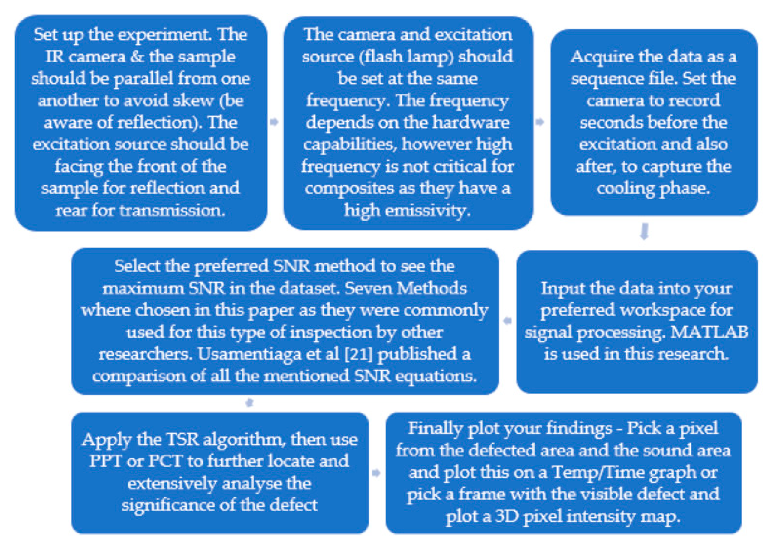
3. Experimental Procedure
3.1. Composites
3.2. Impact Testing
4. Results and Discussion
4.1. Signal Processing
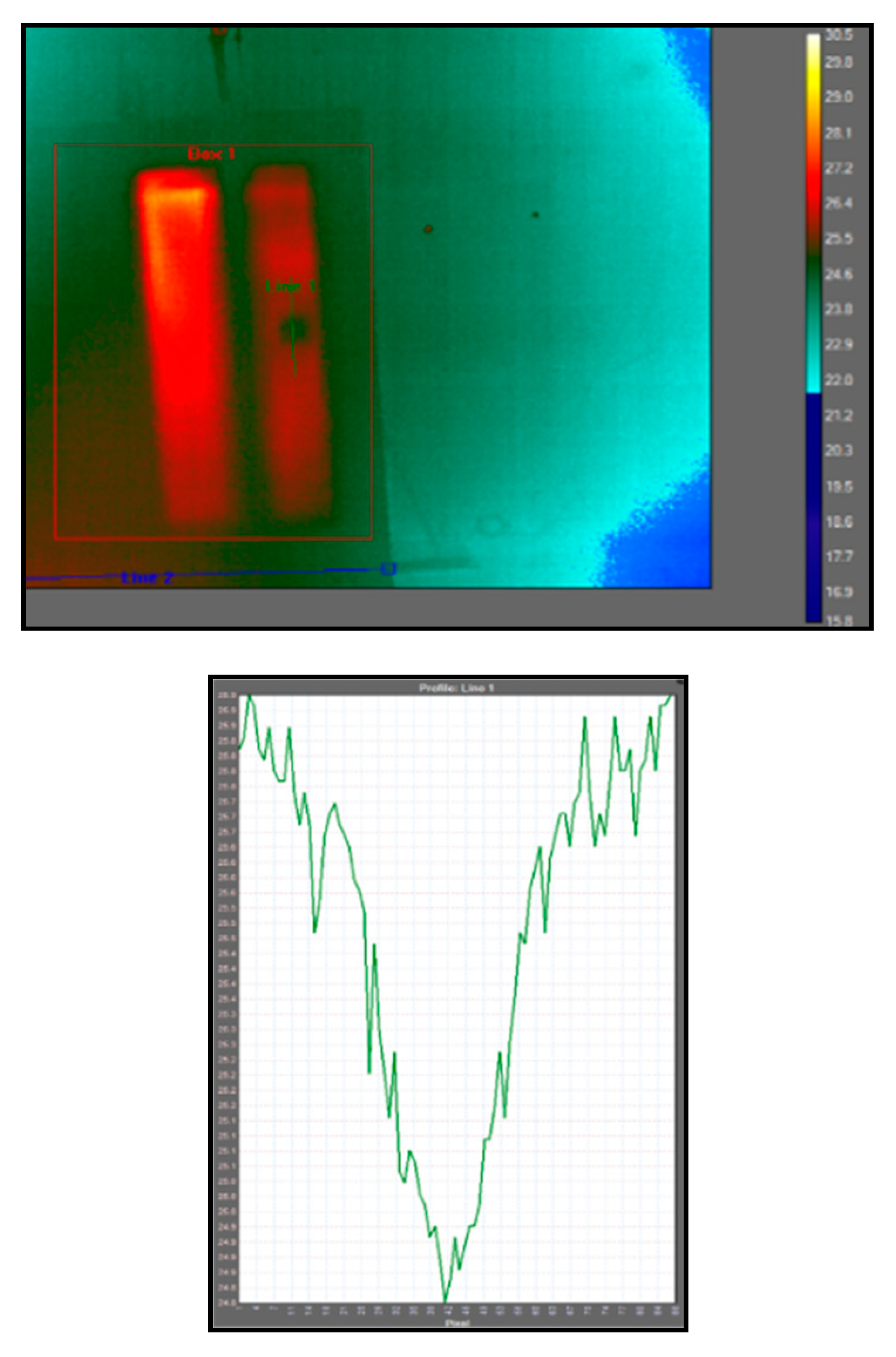
4.1.1. Defect Analysis
4.1.2. Pulsed Phase Thermography (PPT) (Fourier Transform)
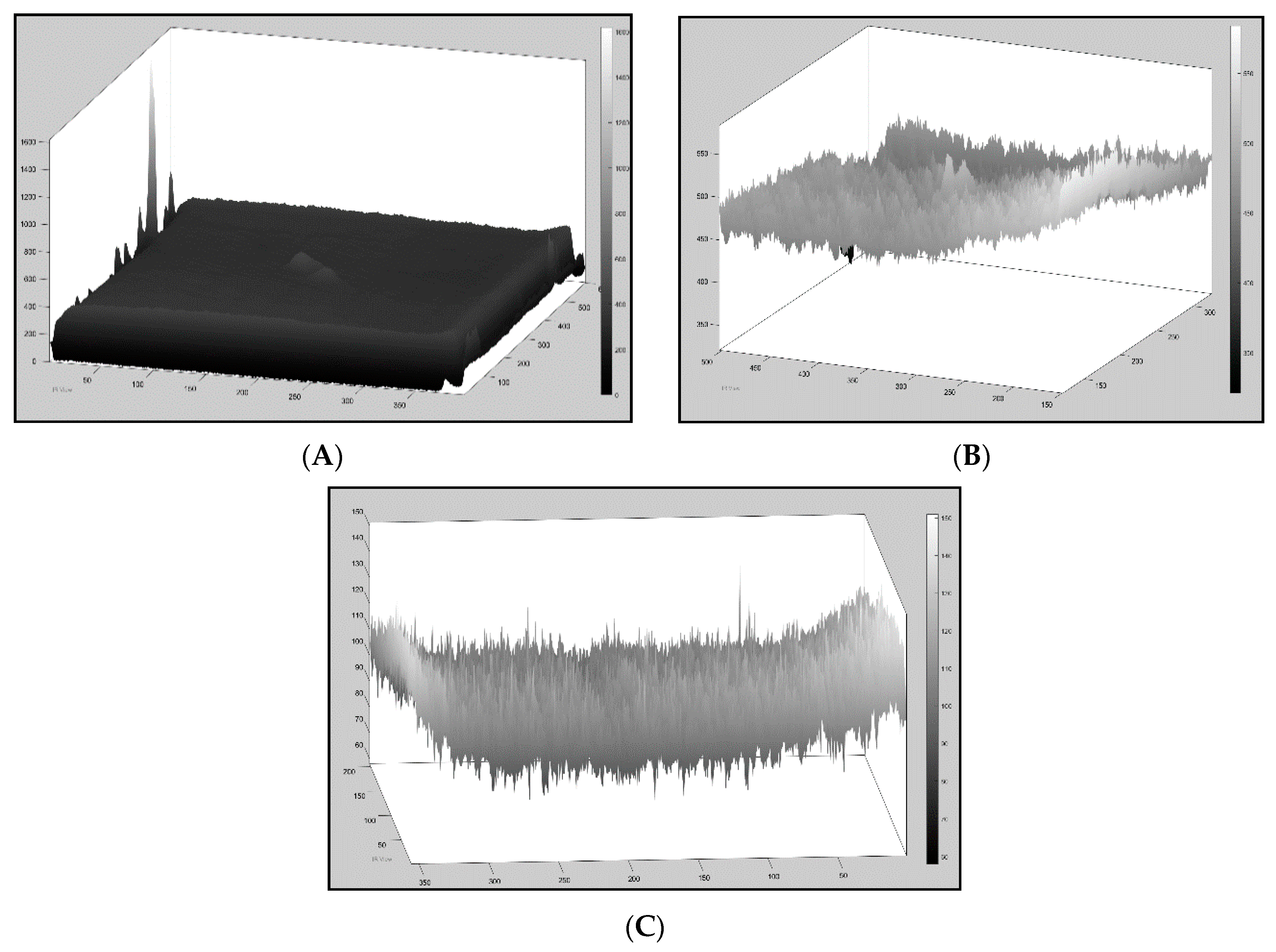
4.1.3. Principal Component Technique (PCT)
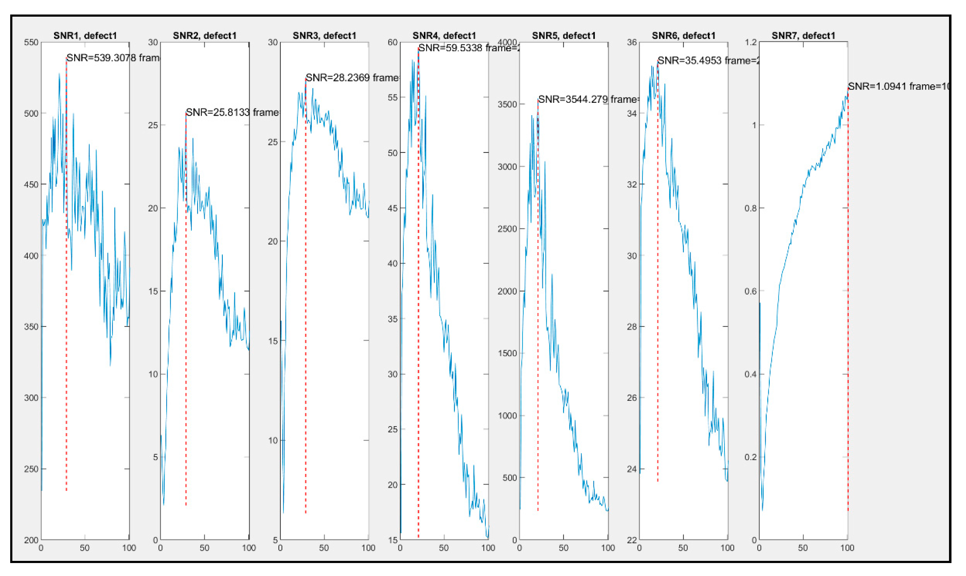
4.1.4. Signal-to-Noise Ratio (SNR)
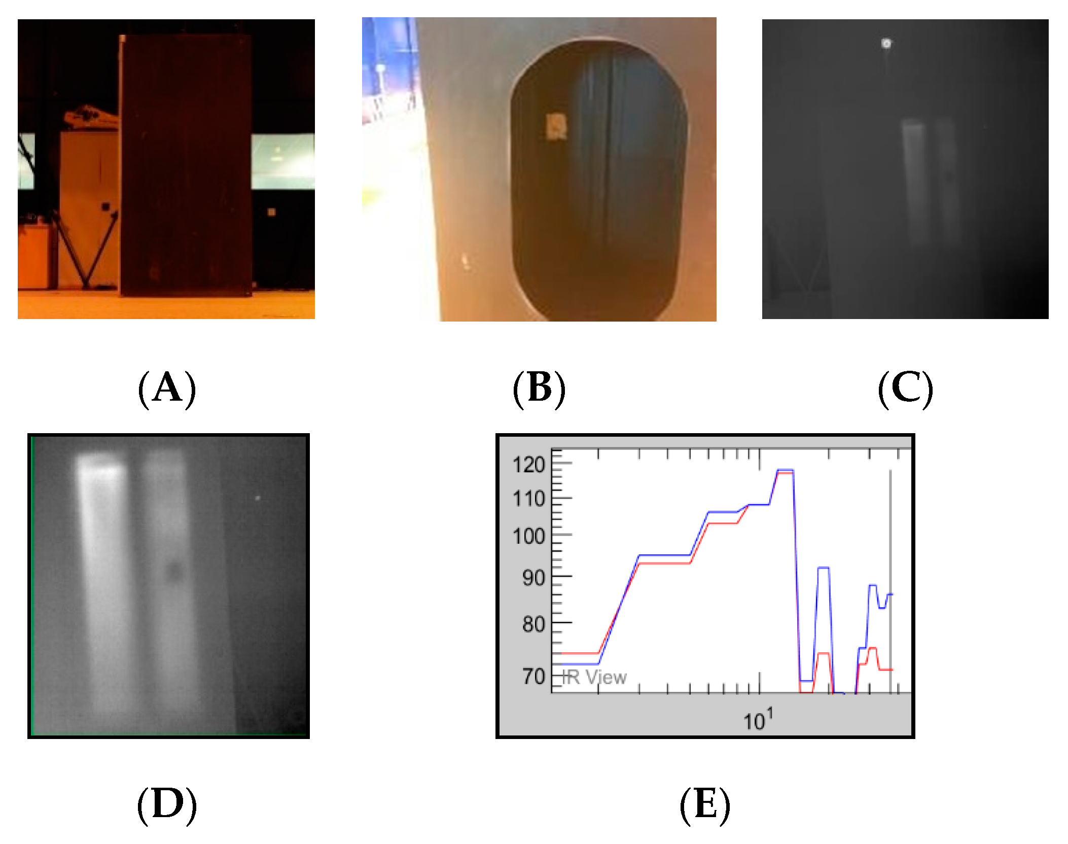
4.2. Active Infrared Thermography
4.3. Signal-to-Noise Ratio Comparison
Interpretation
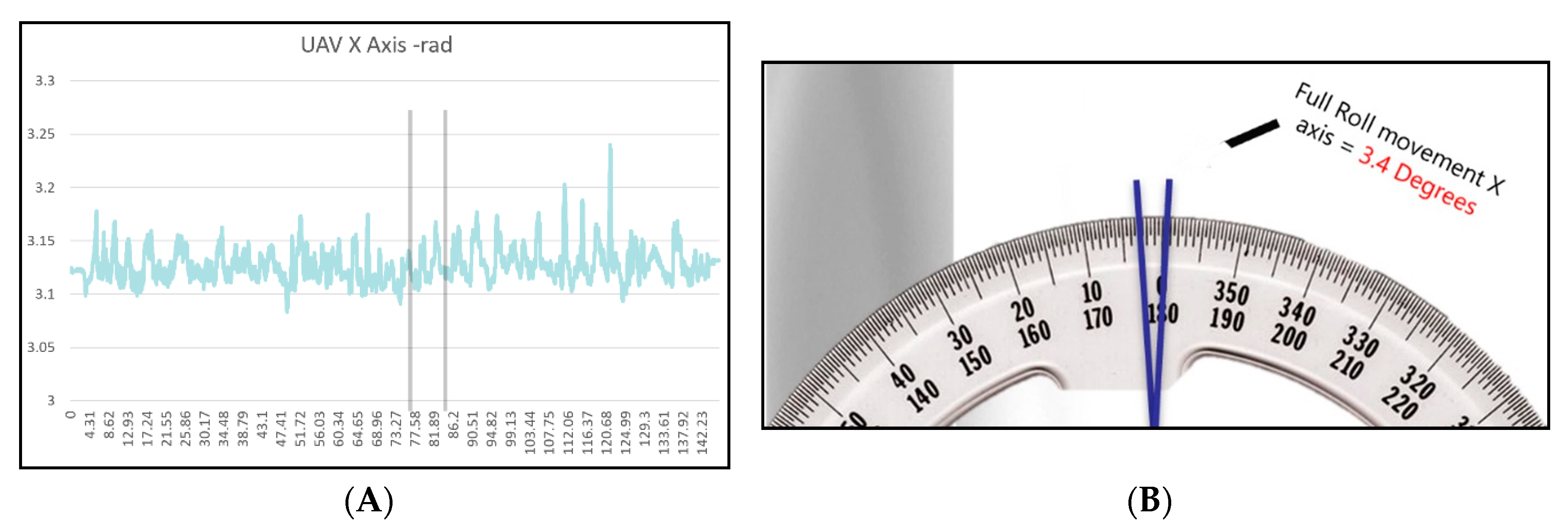
5. UAV Inspection
5.1. Experiment
5.2. Localisation
5.3. NDT Indoor Concept
5.4. NDT Outdoor Concept
6. Conclusions
Author Contributions
Acknowledgments
Conflicts of Interest
Nomenclature
| ε | Emissivity |
| τ | Atmospheric transmittance |
| 1 − ε | Reflectance of the object |
| Atmosphere emissivity | |
| Reflected ambient temperature | |
| The temperature of the atmosphere | |
| Total radiation power received by camera | |
| Wavelength ambient temperature | |
| Wavelength of the object | |
| Wavelength atmosphere | |
| Fe | Flight envelope movement during data capture |
| dE | The position the data capture finished |
| dS | The position the data capture started |
| Specimen location | |
| UAV location | |
| Distance between UAV and specimen |
References
- Hidalgo-Gato García, R.; Andrés Álvarez, J.R.; López Higuera, J.M.; Madruga Saavedra, F.J. Quantification by signal to noise ratio of active infrared thermography data processing techniques. Opt. Photonics J. 2013, 3, 20–26. [Google Scholar] [CrossRef]
- Shrestha, R.; Kim, W. Non-destructive testing and evaluation of materials using active thermography and enhancement of signal to noise ratio through data fusion. Infrared Phys. Technol. 2018, 94, 78–84. [Google Scholar] [CrossRef]
- Fisher, R.; Perkins, S.; Walker, A.; Wolfart, E. Image Transforms—Fourier Transform. 2003. Available online: https://homepages.inf.ed.ac.uk/rbf/HIPR2/fourier.htm (accessed on 12 February 2019).
- Marijke, W.; Rosseel, Y. On the definition of signal-to-noise ratio and contrast-to-noise ratio for fMRI data. PLoS ONE 2013, 8, e77089. [Google Scholar]
- Pasupuleti, D.Y.; Kamalakannan, G.; del Valle, G.G.; Reuter, L.; Dehée, L.; Mestre, L. Cranfield Aerospace Composite Repair. Available online: https://www.researchgate.net/publication/317167462_Cranfield_Aerospace_Composite_Repair_-_Group_Project_Thesis (accessed on 12 February 2019).
- Deane, S.; Avdelidis, N.P.; Ibarra-Castanedo, C.; Zhang, H.; Yazdani Nezhad, H.; Williamson, A.A.; Mackley, T.; Davis, M.J.; Maldague, X.; Tsourdos, A. Application of NDT thermographic imaging of aerospace structures. Infrared Phys. Technol. 2019, 97, 456–466. [Google Scholar] [CrossRef] [Green Version]
- InterNACHI. The History of Infrared Thermography. 2019. Available online: https://www.nachi.org/history-ir.htm (accessed on 12 February 2019).
- Flir System Inc. About Flir Systems. Product Manual, Wilsonville: Omega. 2012. Available online: https://assets.omega.com/manuals/M5230.pdf (accessed on 20 September 2019).
- Rothman, L.S.; Gordon, I.E.; Barbe, A.; Benner, D.C.; Bernath, P.F.; Birk, M.; Boudon, V.; Brown, L.R.; Campargue, A.; Champion, J.P.; et al. The HITRAN 2008 molecular spectroscopic database. J. Quant. Spectros Radiat. Transf. 2009, 110, 533–572. [Google Scholar] [CrossRef] [Green Version]
- Turgut, B.B.; Artan, G.G.; Bek, A. A comparison of MWIR and LWIR imaging systems with regard to range performance. In Infrared Imaging Systems: Design, Analysis, Modeling, and Testing XXIX; SPIE: Orlando, FL, USA, 2018. [Google Scholar]
- Maldague, X.P. Nondestructive Evaluation of Materials by Infrared Thermography; Springer London Limited: Quebec City, QC, Canada, 1992. [Google Scholar]
- FLIR Systems. IR Thermography—How It Works; Techni Tool: Worcester, PA, USA; Available online: http://www.techni-tool.com/site/ARTICLE_LIBRARY/FLIR-IR-Thermography_How-It-Works.pdf (accessed on 13 June 2020).
- Pillans, L.A. Performance Evaluation of an Uncooled Infrared Array Camera. Ph.D. Thesis, University College London, London, UK, 2013. [Google Scholar]
- InfraTec. VarioCAM High Resuolution. Dresden: InfraTec GmbH. 2015. Available online: https://www.infratec.co.uk/downloads/en/thermography/manuals/infratec-manual-variocam-hr.pdf (accessed on 28 September 2019).
- FLIR Systems. ThermaCAM™ Phoenix. Product Manual, Danderyd: FLIR Systems. 2004. Available online: http://www.hoskinscientifique.com/uploadpdf/Instrumentation/FLIR%20Systems/hoskin_phoenix_478b87021a317.pdf (accessed on 20 October 2019).
- Hexcel Corporation. “HexPly® M21.” Hexcel. Available online: https://www.hexcel.com/user_area/content_media/raw/HexPly_M21_global_DataSheet.pdf (accessed on 12 April 2019).
- Nezhad, H.Y.; Merwick, F.; Frizzell, R.M.; McCarthy, C.T. Numerical analysis of low-velocity rigid-body impact response of composite panels. Int. J. Crashworthiness 2014, 20, 27–43. [Google Scholar] [CrossRef]
- Heimbs, S.; Bergmann, T. High-velocity impact behaviour of prestressed composite plates under bird strike loading. Int. J. Aerosp. Eng. 2012, 2012, 372167. [Google Scholar] [CrossRef]
- Gao, Y.; Tian, G.Y. Emissivity correction using spectrum correlation of infrared and visible images. Sens. Actuators 2018, 270, 8–17. [Google Scholar] [CrossRef]
- Duan, Y.; Liu, S.; Hu, C.; Hu, J.; Zhang, H.; Yan, Y.; Tao, N.; Zhang, C.; Maldague, X.; Fang, Q.; et al. Automated defect classification in infrared thermography based on a neural network. NDT E Int. 2019, 107, 102147. [Google Scholar] [CrossRef]
- Shepard, S.M.; Lhota, J.R.; Rubadeux, B.A.; Ahmed, T.; Wang, D. Enhancement and reconstruction of thermographic NDT data. SPIE Int. Soc. Opt. Eng. 2002, 4710, 531–535. [Google Scholar]
- Zhang, H.; Avdelidis, N.P.; Osman, A.; Ibarra-Castanedo, C.; Sfarra, S.; Fernandes, H.; Matikas, T.E.; Maldague, X.P. Enhanced infrared image processing for impacted carbon/glass fiber-reinforced composite evaluation. Sensors 2017, 18, 45. [Google Scholar] [CrossRef] [PubMed] [Green Version]
- Smith, L.I. A tutorial on Principal Components Analysis; Department of Computer Science. Available online: http://www.cs.otago.ac.nz/cosc453/student_tutorials/principal_components.pdf (accessed on 9 December 2019).
- Usamentiaga, R.; Ibarra-Castanedo, C.; Maldague, X. More than fifty shades of grey: Quantitative characterization of defects and interpretation using SNR and CNR. J. Nondestruct. Eval. 2018, 37, 25. [Google Scholar] [CrossRef]
- Usamentiaga, R.; Venegas, P.; Guerediaga, J.; Vega, L.; Molleda, J.; Bulnes, F.G. Infrared thermography for temperature measurement and non-destructive testing. Sensors 2014, 14, 12305–12348. [Google Scholar] [CrossRef] [PubMed] [Green Version]
- Etigowni, S.; Hossain-McKenzie, S.; Kazerooni, M.; Davis, K.; Zonouz, S. Crystal (ball): I Look at Physics and Predict Control Flow! Just-Ahead-Of-Time Controller Recovery. In Proceedings of the 34th Annual Computer Security Applications Conference, San Juan, PR, USA, 3–7 December 2018. [Google Scholar]
- Ciampa, F.; Mahmoodi, P.; Pinto, F.; Meo, M. Recent advances in active infrared thermography for non-destructive testing of aerospace components. Sensors 2018, 18, 609. [Google Scholar] [CrossRef] [PubMed] [Green Version]


| Jenoptik VarioCAM High Resolution | FLIR Phoenix | |
|---|---|---|
| Spectral range | LWIR (7.5–14) μm | MWIR (3–5) μm |
| Pixels | 640 × 480 | 640 × 512 |
| Detector | Uncooled microbolometor FPA | InSb (indium antimonide) FPA |
| Start-up time | <60 s | 10–15 min |
| IR frame rate (full frame) | 50/60 Hz | Up to 90 Hz |
| A/D conversion | 16 bit | 14 bit |
| Power supply | Battery (3 h) | Cabled power supply |
| Vibration resistance in operation | 2 G, IEC 68-2-6 | 6.7 g, RMS random vibe, all 3 axis |
| Size (L × W × H) | (133 × 106 × 110) mm | (190.5 × 111.8 × 132.1) mm |
| Weight | 1.5 kg (completely equipped) | 3.2 kg (excluding lens) |
| Cooling engine | N/A | Stirling closed cycle (~77 K) |
| Noise-equivalent temperature difference (NETD) performance | 70 mK | 25 mK |
| Integration time (electronic shutter speed) | N/A | 9 µs to full frame time |
| Lens | 25-mm lens Field of view = 30° × 23° | 50-mm lens Field of view = 18° × 15° |
| Impact Damage | Energy | Mass | Velocity | Hard/Soft Body Impact |
|---|---|---|---|---|
| Hail in flight | 37 J | 0.001 kg | 37 m/s | Soft |
| Bird strike | 59 kJ | 3.63 kg | 180 m/s | Soft |
| Engine debris | 182 kJ | 2.72 kg | 366 m/s | Hard |
| Rim fragment | 8.4 kJ | 1.68 kg | 100 m/s | Hard |
| Tire fragment | 5.2 kJ | 2.45 kg | 64 m/s | Hard |
| Runway debris | >20 J | 0.01 kg | >60 m/s | Hard |
| Tool drop | 28 J | 0.56 kg | 10 m/s | Hard |
| Hail on ground | 100 J | 0.113 kg | 42 m/s | Hard |
| Ply Mass | Ply Thickness | Fibre Volume Fraction | ILSS |
|---|---|---|---|
| 305 g/m2 | 0.262 mm | 56.6% | 60 MPa |
| Tensile strength | Tensile modulus | GIc | GIIc |
| 3039 MPa | 172 GPa | 765 J/m2 | 1250 J/m2 |
© 2020 by the authors. Licensee MDPI, Basel, Switzerland. This article is an open access article distributed under the terms and conditions of the Creative Commons Attribution (CC BY) license (http://creativecommons.org/licenses/by/4.0/).
Share and Cite
Deane, S.; Avdelidis, N.P.; Ibarra-Castanedo, C.; Zhang, H.; Nezhad, H.Y.; Williamson, A.A.; Mackley, T.; Maldague, X.; Tsourdos, A.; Nooralishahi, P. Comparison of Cooled and Uncooled IR Sensors by Means of Signal-to-Noise Ratio for NDT Diagnostics of Aerospace Grade Composites. Sensors 2020, 20, 3381. https://0-doi-org.brum.beds.ac.uk/10.3390/s20123381
Deane S, Avdelidis NP, Ibarra-Castanedo C, Zhang H, Nezhad HY, Williamson AA, Mackley T, Maldague X, Tsourdos A, Nooralishahi P. Comparison of Cooled and Uncooled IR Sensors by Means of Signal-to-Noise Ratio for NDT Diagnostics of Aerospace Grade Composites. Sensors. 2020; 20(12):3381. https://0-doi-org.brum.beds.ac.uk/10.3390/s20123381
Chicago/Turabian StyleDeane, Shakeb, Nicolas P. Avdelidis, Clemente Ibarra-Castanedo, Hai Zhang, Hamed Yazdani Nezhad, Alex A. Williamson, Tim Mackley, Xavier Maldague, Antonios Tsourdos, and Parham Nooralishahi. 2020. "Comparison of Cooled and Uncooled IR Sensors by Means of Signal-to-Noise Ratio for NDT Diagnostics of Aerospace Grade Composites" Sensors 20, no. 12: 3381. https://0-doi-org.brum.beds.ac.uk/10.3390/s20123381