Comparative Analysis on Machine Learning and Deep Learning to Predict Post-Induction Hypotension

 , , ,
, , ,
Abstract
:1. Introduction
Related Work
2. Materials and Methods
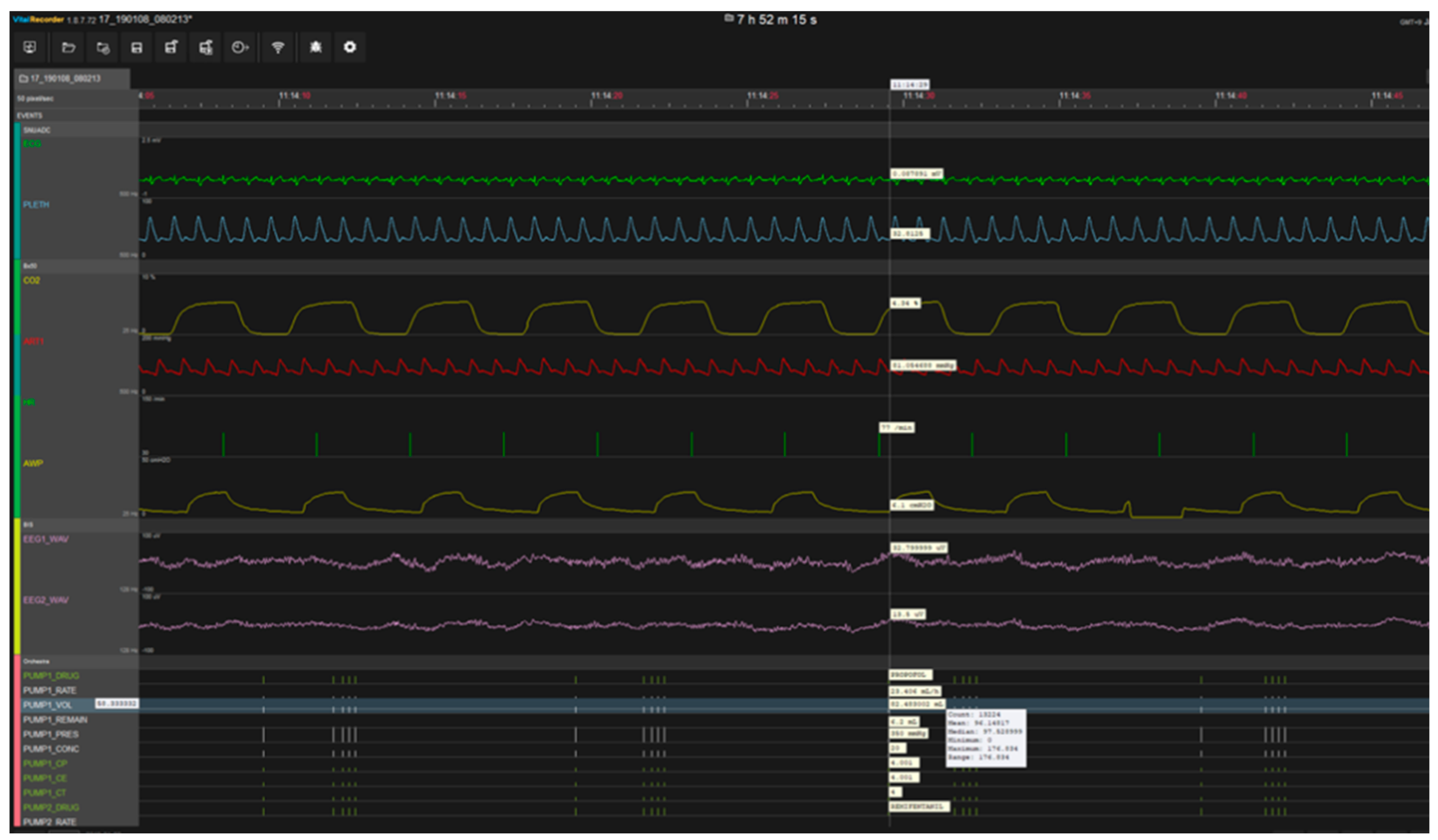
2.1. Data Collection
2.2. Features
2.3. Algorithms
2.4. Problem Definition and Labeling Approach
2.5. Model Building
2.6. Performance Evaluation
3. Results
4. Discussion
Author Contributions
Funding
Conflicts of Interest
Appendix A

| All Features (106) | Feature Set A (45) | Feature Set B (20) | Feature Set C (29) |
|---|---|---|---|
| Age | 〮 | 〮 | 〮 |
| Sex | 〮 | ||
| Height | 〮 | ||
| Weight | 〮 | ||
| Body mass index | 〮 | ||
| ASA classification | |||
| Comorbidities | |||
| Cardiovascular disease | |||
| Hypertension | 〮 | ||
| Atrial fibrillation | |||
| Coronary artery disease | 〮 | ||
| Angina pectoris | 〮 | ||
| Congestive heart failure | 〮 | ||
| Valvular heart disease | 〮 | ||
| Respiratory disease | |||
| Asthma | 〮 | ||
| Chronic obstructive pulmonary disease | 〮 | ||
| Gastrointestinal disease | |||
| Hepatitis | 〮 | ||
| Liver cirrhosis | 〮 | ||
| Viral carrier | |||
| Hepatitis B viral infection | 〮 | ||
| Hepatitis C viral infection | 〮 | ||
| Renal disease | |||
| Chronic kidney injury | 〮 | ||
| End-stage renal disease | 〮 | ||
| Endocrine disease | |||
| Diabetes mellitus | |||
| HbA1c | 〮 | ||
| Thyroid disease | 〮 | ||
| Neurologic disease | |||
| Cerebrovascular disease | 〮 | ||
| Cerebral aneurysm | 〮 | ||
| Baseline blood pressure -mmHg | |||
| Systolic | 〮 | 〮 | |
| Mean | 〮 | 〮 | 〮 |
| Diastolic | 〮 | 〮 | |
| Noninvasive blood pressure | |||
| Systolic min | 〮 | 〮 | |
| Systolic max | 〮 | ||
| Systolic mean | 〮 | 〮 | |
| Systolic sd | |||
| Mean min | 〮 | 〮 | |
| Mean max | 〮 | ||
| Mean mean | 〮 | 〮 | |
| Mean sd | 〮 | ||
| Diastolic min | 〮 | ||
| Diastolic max | 〮 | ||
| Diastolic mean | 〮 | ||
| Diastolic sd | 〮 | ||
| Heart rate | |||
| min | |||
| max | |||
| mean | 〮 | 〮 | |
| Mechanical ventilation data | |||
| Respiratory rate min | |||
| Respiratory rate max | 〮 | ||
| Respiratory rate mean | 〮 | ||
| Tidal volume min | 〮 | 〮 | 〮 |
| Tidal volume max | 〮 | 〮 | |
| Tidal volume mean | |||
| Minute ventilation min | 〮 | ||
| Minute ventilation max | |||
| Minute ventilation mean | |||
| Peak inspiratory pressure min | 〮 | ||
| Peak inspiratory pressure max | 〮 | ||
| Peak inspiratory pressure mean | 〮 | 〮 | |
| Anesthetic drug | |||
| Rate | |||
| propofol min | 〮 | 〮 | 〮 |
| propofol max | 〮 | ||
| propofol mean | 〮 | ||
| Remifentanil min | 〮 | 〮 | |
| Remifentanil max | 〮 | 〮 | |
| Remifentanil mean | 〮 | 〮 | |
| Plasma concentration | |||
| propofol min | 〮 | 〮 | |
| propofol max | 〮 | ||
| propofol mean | |||
| Remifentanil min | |||
| Remifentanil max | |||
| Remifentanil mean | |||
| Effect-site concentration | |||
| propofol min | |||
| propofol max | 〮 | 〮 | |
| propofol mean | |||
| Remifentanil min | |||
| Remifentanil max | |||
| Remifentanil mean | |||
| Target concentration | |||
| propofol min | |||
| propofol max | |||
| propofol mean | |||
| Remifentanil min | 〮 | ||
| Remifentanil max | |||
| Remifentanil mean | |||
| Volume | |||
| propofol min | 〮 | 〮 | |
| propofol max | |||
| propofol mean | 〮 | ||
| Remifentanil min | 〮 | 〮 | 〮 |
| Remifentanil max | 〮 | ||
| Remifentanil mean | 〮 | 〮 | |
| Vasoactive drug administration | |||
| Ephedrine | |||
| Ephedrine volume | 〮 | ||
| Phenylephrine | 〮 | ||
| Phenylephrine volume | |||
| Nicardipine | 〮 | ||
| Nicardipine volume | |||
| Esmolol | 〮 | ||
| Esmolol volume | |||
| Hypotension | |||
| Frequency | 〮 | ||
| Duration | 〮 | ||
| Average duration | 〮 | 〮 |
References
- Monk, T.G.; Bronsert, M.R.; Henderson, W.G.; Mangione, M.P.; Sum-Ping, S.T.J.T.; Bentt, D.R.; Nguyen, J.D.; Richman, J.S.; Meguid, R.A.; Hammermeister, K.E. Association between Intraoperative Hypotension and Hypertension and 30-day Postoperative Mortality in Noncardiac Surgery. Anesthesiology 2015, 123, 307–319. [Google Scholar] [CrossRef] [PubMed]
- Bijker, J.B.; Van Klei, W.A.; Vergouwe, Y.; Eleveld, D.J.; Van Wolfswinkel, L.; Moons, K.G.M.; Kalkman, C.J. Intraoperative Hypotension and 1-Year Mortality after Noncardiac Surgery. Anesthesiology 2009, 111, 1217–1226. [Google Scholar] [CrossRef] [PubMed] [Green Version]
- Sun, L.; Wijeysundera, D.N.; Tait, G.; Beattie, W.S. Association of Intraoperative Hypotension with Acute Kidney Injury after Elective Noncardiac Surgery. Anesthesiology 2015, 123, 515–523. [Google Scholar] [CrossRef] [PubMed]
- Walsh, M.; Devereaux, P.J.; Garg, A.X.; Kurz, A.; Turan, A.; Rodseth, R.N.; Sessler, D.I. Relationship between intraoperative mean arterial pressure and clinical outcomes after noncardiac SurgeryToward an empirical definition of hypotension. Anesthesiol. J. Am. Soc. Anesthesiol. 2013, 119, 507–515. [Google Scholar]
- Daugirdas, J.T. Dialysis hypotension: A hemodynamic analysis. Kidney Int. 1991, 39, 233–246. [Google Scholar] [CrossRef] [Green Version]
- Cavalcanti, S.; Ciandrini, A.; Severi, S.; Badiali, F.; Bini, S.; Gattiani, A.; Cagnoli, L.; Santoro, A.; Cavalcanti, A.C.S. Model-based study of the effects of the hemodialysis technique on the compensatory response to hypovolemia. Kidney Int. 2004, 65, 1499–1510. [Google Scholar] [CrossRef] [PubMed] [Green Version]
- Shoji, T.; Tsubakihara, Y.; Fujii, M.; Imai, E. Hemodialysis-associated hypotension as an independent risk factor for two-year mortality in hemodialysis patients. Kidney Int. 2004, 66, 1212–1220. [Google Scholar] [CrossRef] [Green Version]
- Kendale, S.; Kulkarni, P.; Rosenberg, A.D.; Wang, J. Supervised Machine-learning Predictive Analytics for Prediction of Postinduction Hypotension. Anesthesiology 2018, 129, 675–688. [Google Scholar] [CrossRef]
- Hatib, F.; Jian, Z.; Buddi, S.; Lee, C.; Settels, J.; Sibert, K.; Rinehart, J.; Cannesson, M. Machine-learning Algorithm to Predict Hypotension Based on High-fidelity Arterial Pressure Waveform Analysis. Anesthesiology 2018, 129, 663–674. [Google Scholar] [CrossRef]
- Kang, A.R.; Lee, J.; Jung, W.; Lee, M.; Park, S.Y.; Woo, J.; Kim, S.H. Development of a prediction model for hypotension after induction of anesthesia using machine learning. PLoS ONE 2020, 15, e0231172. [Google Scholar] [CrossRef] [Green Version]
- Lee, H.-C.; Jung, C.-W. Vital Recorder—A free research tool for automatic recording of high-resolution time-synchronised physiological data from multiple anaesthesia devices. Sci. Rep. 2018, 8, 1527. [Google Scholar] [CrossRef] [PubMed] [Green Version]
- Ko, B.S.; Kim, Y.-J.; Jung, D.H.; Sohn, C.H.; Seo, D.W.; Lee, Y.-S.; Lim, K.S.; Jung, H.-Y.; Kim, W.Y. Early Risk Score for Predicting Hypotension in Normotensive Patients with Non-Variceal Upper Gastrointestinal Bleeding. J. Clin. Med. 2019, 8, 37. [Google Scholar] [CrossRef] [PubMed] [Green Version]
- Lee, K.; Jang, J.S.; Kim, J.; Suh, Y.J. Age shock index, shock index, and modified shock index for predicting postintubation hypotension in the emergency department. Am. J. Emerg. Med. 2020, 38, 911–915. [Google Scholar] [CrossRef] [PubMed]
- Reich, D.; Hossain, S.; Krol, M.; Baez, B.; Patel, P.; Bernstein, A.; Bodian, C.A. Predictors of Hypotension After Induction of General Anesthesia. Anesthesia Analg. 2005, 101, 622–628. [Google Scholar] [CrossRef] [PubMed]
- Südfeld, S.; Brechnitz, S.; Wagner, J.Y.; Reese, P.C.; Pinnschmidt, H.O.; Reuter, D.A.; Saugel, B. Post-induction hypotension and early intraoperative hypotension associated with general anaesthesia. Br. J. Anaesth. 2017, 119, 57–64. [Google Scholar] [CrossRef] [Green Version]
- Nonaka, T.; Oka, S.; Miyata, K.; Mikami, T.; Koyanagi, I.; Houkin, K.; Yoshifuji, K.; Imaizumi, T. Prediction of Prolonged Postprocedural Hypotension after Carotid Artery Stenting. Neurosurgery 2005, 57, 472–477. [Google Scholar] [CrossRef]
- Ghosh, S.; Feng, M.; Nguyen, H.T.; Li, J. Hypotension Risk Prediction via Sequential Contrast Patterns of ICU Blood Pressure. IEEE J. Biomed. Health Inform. 2015, 20, 1416–1426. [Google Scholar] [CrossRef]
- Janghorbani, A.; Arasteh, A.; Moradi, M.H. Prediction of acute hypotension episodes using Logistic Regression model and Support Vector Machine: A comparative study. In Proceedings of the 19th Iranian Conference on Electrical Engineering, Tehran, Iran, 17–19 May 2011; pp. 1–4. [Google Scholar]
- Park, S.; Kim, W.-J.; Cho, N.-J.; Choi, C.-Y.; Heo, N.H.; Gil, H.-W.; Lee, E.Y. Predicting intradialytic hypotension using heart rate variability. Sci. Rep. 2019, 9, 2574. [Google Scholar] [CrossRef] [Green Version]
- Moghadam, M.C.; Abad, E.M.K.; Bagherzadeh, N.; Ramsingh, D.; Li, G.-P.; Kain, Z.N.; Masoumi, E. A machine-learning approach to predicting hypotensive events in ICU settings. Comput. Boil. Med. 2020, 118, 103626. [Google Scholar] [CrossRef]
- Lin, C.-S.; Chiu, J.-S.; Hsieh, M.-H.; Mok, M.S.; Li, Y.-C. (Jack); Chiu, H.W. Predicting hypotensive episodes during spinal anesthesia with the application of artificial neural networks. Comput. Methods Programs Biomed. 2008, 92, 193–197. [Google Scholar] [CrossRef]
- Lee, H.C.; Ryu, H.G.; Chung, E.J.; Jung, C.W. Prediction of Bispectral Index during Target-controlled Infusion of Propofol and RemifentanilA Deep Learning Approach. Anesthesiol. J. Am. Soc. Anesthesiol. 2018, 128, 492–501. [Google Scholar]
- Breiman, L.; Last, M.; Rice, J. Random Forests: Finding Quasars. Stat. Chall. Astron. 2006, 45, 243–254. [Google Scholar] [CrossRef]
- Chen, T.; Guestrin, C. Xgboost: A scalable tree boosting system. In Proceedings of the 22nd ACM Sigkdd International Conference on Knowledge Discovery and Data Mining, San Francisco, CA, USA, 13–17 August 2016; pp. 785–794. [Google Scholar]
- Chen, J.-B.; Wu, K.-C.; Moi, S.-H.; Chuang, L.-Y.; Yang, C.-H. Deep Learning for Intradialytic Hypotension Prediction in Hemodialysis Patients. IEEE Access 2020, 8, 82382–82390. [Google Scholar] [CrossRef]
- LeCun, Y.; Bottou, L.; Bengio, Y.; Haffner, P. Gradient-based learning applied to document recognition. Proc. IEEE 1998, 86, 2278–2324. [Google Scholar] [CrossRef] [Green Version]
- Hannun, A.; Rajpurkar, P.; Haghpanahi, M.; Tison, G.H.; Bourn, C.; Turakhia, M.P.; Ng, A.Y. Cardiologist-level arrhythmia detection and classification in ambulatory electrocardiograms using a deep neural network. Nat. Med. 2019, 25, 65–69. [Google Scholar] [CrossRef] [PubMed]
- Jain, A.; Zongker, D. Feature selection: Evaluation, application, and small sample performance. IEEE Trans. Pattern Anal. Mach. Intell. 1997, 19, 153–158. [Google Scholar] [CrossRef] [Green Version]
- Powers, D.M. Evaluation: From precision, recall and F-measure to ROC, informedness, markedness and correlation. J. Mach. Learn. Technol. 2011, 2, 37–63. [Google Scholar]
- Archer, K.J.; Kimes, R.V. Empirical characterization of random forest variable importance measures. Comput. Stat. Data Anal. 2008, 52, 2249–2260. [Google Scholar] [CrossRef]
- Convertino, V.A.; Moulton, S.L.; Grudic, G.Z.; Rickards, C.A.; Hinojosa-Laborde, C.; Gerhardt, R.T.; Blackbourne, L.H.; Ryan, K.L. Use of Advanced Machine-Learning Techniques for Noninvasive Monitoring of Hemorrhage. J. Trauma Inj. Infect. Crit. Care 2011, 71, S25–S32. [Google Scholar] [CrossRef]
- Volak, J.; Bajzik, J.; Janisova, S.; Koniar, D.; Hargas, L. Real-Time Interference Artifacts Suppression in Array of ToF Sensors. Sensors 2020, 20, 3701. [Google Scholar] [CrossRef]
- Matsuo, K.; Aihara, H.; Nakai, T.; Morishita, A.; Tohma, Y.; Kohmura, E. Machine Learning to Predict In-Hospital Morbidity and Mortality after Traumatic Brain Injury. J. Neurotrauma 2020, 37, 202–210. [Google Scholar] [CrossRef] [PubMed]
- Lee, C.K.; Hofer, I.; Gabel, E.; Baldi, P.; Cannesson, M. Development and validation of a deep neural network model for prediction of postoperative in-hospital mortality. Anesthesiology 2018, 129, 649–662. [Google Scholar] [CrossRef] [PubMed]
- Lee, H.; Shin, S.-Y.; Seo, M.; Nam, G.-B.; Joo, S. Prediction of Ventricular Tachycardia One Hour before Occurrence Using Artificial Neural Networks. Sci. Rep. 2016, 6, 32390. [Google Scholar] [CrossRef]
- Jeong, Y.-S.; Kang, A.R.; Jung, W.; Lee, S.J.; Lee, S.; Lee, M.; Chung, Y.H.; Koo, B.S.; Kim, S.H. Prediction of Blood Pressure after Induction of Anesthesia Using Deep Learning: A Feasibility Study. Appl. Sci. 2019, 9, 5135. [Google Scholar] [CrossRef] [Green Version]


| Study | Outcome | Outcome Type | Feature | Algorithm | Performance |
|---|---|---|---|---|---|
| Park et al. [19] | Hypotension before 1 month after surgery for hemodialysis patients | Static, after surgery | Heart rate variability (DM, CAD, CHF, Age, UFR, iPTH, ARB or ACEI, CCB, b-blocker, Mean HR, RRI, SDNN, RMSSD, VLF, LF, HF, TP, LF/HF ratio) | Multivariate negative binomial model | AUC: 0.804 |
| Moghadam et al. [20] | At least 5 min before hypotension | Dynamic | ABP (arterial blood pressure), HR, Sys, Dia, Resp, SpO2, PP, MAP, CO, MAP to HR ratio (MAP2HR), average of RR intervals on ECG time series (RR) | Logistic Regression (LR) | Accuracy: 95% Sensitivity: 85% Specificity: 96% |
| Kendale et al. [8] | Hypotension within 10 min after induction | Static, at induction | Age, Sex, BMI, ASA Score, Medical comorbidities, Preoperative medication, Intraoperative medications, Mean peak inspiratory pressure, First mean arterial pressure, Time of day, non-invasive and invasive blood pressure | LR, Support Vector Machine, Naïve Bayes, K-Nearest Neighbor, Linear Discriminant Analysis, Random Forest, Neural Network, Gradient Boosting Algorithm | Sensitivity: 64% Specificity: 75% AUC: 0.76 |
| Lin et al. [21] | Hypotension within 15 min after induction for spinal anesthesia | Static, at induction | Age, Gender, Weight, Height, Hematocrit, ASA score, Basal SBP, Basal DBP, Basal HR, History of hypertension, History of diabetes, Surgical category, Emergency, Dose of local anesthetics | LR, ANN, Simplified ANN | Accuracy: 77.6% Sensitivity: 75.9% Specificity: 76% |
| Hatib et al. [9] | Hypotension at least within 5 min | Dynamic | 3022 features from arterial pressure waveform: Signal features, floTrac features, COTrek features, complexity features, Baroeflex features, variability features, spectral features, Delta change features | LR | Sensitivity: 86.8% Specificity: 88.5% AUC: 0.95 |
| Data Source | Categories | Features |
|---|---|---|
| Electronic Health Record | Demographic data | Age Sex Height Weight Body mass index ASA classification Base Systolic Blood Pressure Base Diastolic Blood Pressure Base Mean Blood Pressure |
| Comorbidities | Cardiovascular disease | |
| Respiratory disease | ||
| Gastrointestinal disease | ||
| Renal disease | ||
| Endocrine disease | ||
| Neurologic disease | ||
| Baseline | Systolic | |
| Mean | ||
| Diastolic | ||
| Vital Recorder | Noninvasive blood pressure | Systolic |
| Mean | ||
| Diastolic | ||
| Heart rate | Heart rate | |
| Mechanical ventilation data | Plethysmogram oxygen saturation | |
| End-tidal CO2 partial pressure | ||
| NMT_TOF_CNT | ||
| Respiratory rate | ||
| Tidal volume | ||
| Minute ventilation | ||
| Peak inspiratory pressure | ||
| Positive end expiratory pressure | ||
| Bispectral index | Spectral edge frequency | |
| Signal quality index | ||
| Electromyogram power | ||
| Total power | ||
| Bispectral index value | ||
| Anesthetic drug | Rate | |
| Plasma concentration | ||
| Effect-site concentration | ||
| Target concentration | ||
| Volume | ||
| Vasoactive drug administration | Vasopressor | |
| Vasodilator | ||
| Hypotension | Frequency | |
| Duration | ||
| Average duration |
| Characteristic | All Patients (n = 82) | Hypotension (n = 151) | Non Hypotension (n = 131) | p-Value |
|---|---|---|---|---|
| Age | 54.7 (14.1) | 56.5 (14.5) | 52.6 (13.4) | 0.023 * |
| Sex (male) | 134 (47.5%) | 66 (43.7%) | 68 (51.9%) | 0.209 |
| Height | 162.1 (9) | 161.2 (8.7) | 163.2 (9.2) | 0.067 |
| Weight | 66.6 (12.4) | 64.5 (12) | 69.2 (12.5) | 0.002 ** |
| BMI | 25.2 (3.6) | 24.7 (3.6) | 25.8 (3.5) | 0.019 * |
| ASA classification -no | 0.426 | |||
| 1 | 95 (33.7%) | 48 (31.8%) | 47 (35.9%) | |
| 2 | 151 (54.6%) | 82 (54.3%) | 72 (55%) | |
| 3 | 33 (11.7%) | 21 (13.9%) | 12 (9.1%) | |
| Comorbidities | ||||
| Cardiovascular disease | ||||
| Hypertension | 97 (34.4%) | 55 (36.4%) | 42 (32.1%) | 0.520 |
| Atrial fibrillation | 2 (0.7%) | 2 (1.3%) | 0 | 0.500 |
| Coronary artery disease | 5 (1.8%) | 4 (2.6%) | 1 (0.8%) | 0.377 |
| Angina pectoris | 5 (1.8%) | 2 (1.3%) | 3 (2.3%) | 0.666 |
| Congestive heart failure | 1 (0.4%) | 1 (0.7%) | 1 (0.8%) | 1.000 |
| Valvular heart disease | 1 (0.4%) | 1 (0.7%) | 0 | 1.000 |
| Respiratory disease | ||||
| Asthma | 17 (6%) | 14 (9.3%) | 3 (2.3%) | 0.027* |
| Chronic obstructive pulmonary disease | 6 (2.1%) | 3 (2%) | 3 (2.3%) | 1.000 |
| Gastrointestinal disease | ||||
| Hepatitis | 3 (1.1%) | 2 (1.3%) | 1 (0.8%) | 1.000 |
| Liver cirrhosis | 6 (2.1%) | 3 (2%) | 3 (2.3%) | 1.000 |
| Viral carrier | 6 (2.1%) | 3 (2%) | 3 (2.3%) | 1.000 |
| Hepatitis B viral infection | 12 (4.3%) | 5 (3.3%) | 7 (5.3%) | 0.584 |
| Hepatitis C viral infection | 2 (0.7%) | 1 (0.7%) | 1 (0.8%) | 1.000 |
| Renal disease | ||||
| Chronic kidney injury | 0.209 | |||
| 2 | 1 (0.4%) | 0 | 1 (0.8%) | |
| 3 | 3 (1.1%) | 3 (2%) | 0 | |
| 4 | 1 (0.4%) | 1 (0.7%) | 0 | |
| End-stage renal disease | 1 (0.4%) | 1 (0.7%) | 0 | 1.000 |
| Endocrine disease | ||||
| Diabetes mellitus | 62 (22%) | 37 (24.5%) | 25 (19.1%) | 0.341 |
| Thyroid disease | 0.667 | |||
| 1 | 3 (1.1%) | 2 (1.3%) | 1 (0.8%) | |
| 2 | 4 (1.4%) | 1 (0.7%) | 3 (2.3%) | |
| 3 | 8 (2.8%) | 5 (3.3%) | 3 (2.3%) | |
| Neurologic disease | ||||
| Cerebrovascular disease | 12 (4.3%) | 8 (5.350 | 4 (3.1%) | 0.525 |
| Cerebral aneurysm | 1 (0.4%) | 0 | 1 (0.8%) | 0.465 |
| Baseline blood pressure -mmHg | ||||
| Systolic | 146.2 (23.8) | 140.8 (23.1) | 152.3 (23.1) | 0.001 *** |
| Mean | 105.9 (16) | 102.4 (16.2) | 109.9 (15) | 0.001 *** |
| Diastolic | 80.9 (10.5) | 78.3 (10.5) | 83.9 (9.8) | 0.001 *** |
| Noninvasive blood pressure -mmHg | ||||
| Systolic | 113.3 (22.7) | 105.4 (18.1) | 122.3 (24) | <0.001 *** |
| Mean | 84.3 (15.5) | 78.9 (12.5) | 90.4 (16.2) | <0.001 *** |
| Diastolic | 66.6 (12.5) | 62.7 (10.8) | 71.2 (12.8) | <0.001 *** |
| Heart rate -/min | 70.6 (13.1) | 70.8 (12.9) | 70.3 (13.3) | <0.001 |
| Mechanical ventilation data | ||||
| Plethysmogram oxygen saturation | 99.4 (1.5) | 99.4 (1.7) | 99.4 (1.5) | <0.001 *** |
| End-tidal CO2 partial pressure -% | 2.5 (1.5) | 2.5 (1.5) | 2.4 (1.5) | 0.001 *** |
| NMT_TOF_CNT | 2 (1.9) | 2.1 (1.9) | 1.9 (1.9) | 0.001 *** |
| Respiratory rate -/min | 15.7 (8.5) | 15.8 (8.6) | 15.5 (8.4) | 0.210 |
| Tidal volume -mL | 242.4 (172.3) | 242.3 (168.8) | 242.5 (176.2) | 0.318 |
| Minute ventilation -L/min | 4.2 (2.7) | 4.2 (2.7) | 4.2 (2.8) | 0.169 |
| Peak inspiratory pressure -cmH2O | 16.5 (7.4) | 16.1 (7) | 16.9 (7.7) | <0.001 *** |
| Positive end expiratory pressure -cmH2O | 3.1 (2.3) | 3.1 (2.2) | 3.1 (2.3) | 0.480 |
| Bispectral index | ||||
| Spectral edge frequency -Hz | 17.1 (3.7) | 17.1 (3.7) | 17 (3.7) | 0.001 *** |
| Signal quality index -Hz | 87.4 (16.2) | 88.6 (15.3) | 86.1 (17.2) | <0.001 *** |
| Electromyogram power -Hz | 30.5 (6.8) | 30.1 (6.4) | 30.9 (7.3) | 0.001 *** |
| Total power | 63 (7.5) | 63 (7.5) | 63.1 (7.4) | 0.007** |
| Bispectral index value | 51.8 (16.6) | 52.2 (16) | 51.5 (17.3) | 0.001 *** |
| Anesthetic drug | ||||
| Rate | ||||
| propofol -mg | 52.6 (91.4) | 47.6 (60.2) | 58.4 (117.2) | <0.001 *** |
| remifentanil -mg | 8.3 (33.6) | 7.2 (30.2) | 9.5 (37.2) | 0.001 *** |
| Plasma concentration | ||||
| propofol -mg | 5.3 (2.2) | 5.2 (2) | 5.4 (2.4) | <0.001 *** |
| remifentanil -mg | 2.1 (1.7) | 2.1 (1.6) | 2.2 (1.8) | 0.001 *** |
| Effect-site concentration | ||||
| propofol -mg | 4.9 (1.1) | 4.9 (0.9) | 4.9 (1.2) | <0.001 *** |
| remifentanil -mg | 1.7 (0.9) | 1.6 (0.9) | 1.7 (0.9) | <0.001 *** |
| Target concentration | ||||
| propofol -mg | 4.9 (1) | 4.9 (0.9) | 4.9 (1.1) | <0.001 *** |
| remifentanil -mg | 1.6 (1) | 1.5 (1) | 1.6 (1.1) | 0.001 *** |
| Volume | ||||
| propofol -mg | 6.7 (2.5) | 6.4 (4.9) | 7 (3) | <0.001 *** |
| remifentanil -mg | 0.8 (0.7) | 0.7 (0.4) | 0.9 (1) | <0.001 *** |
| Vasoactive drug administration -no | ||||
| Ephedrine | 4 (1.4%) | 4 (2.6%) | 0 | 0.126 |
| Phenylephrine | 1 (0.4%) | 1 (0.7%) | 0 | 1.000 |
| Nicardipine | 1 (0.4%) | 0 | 1 (0.8%) | 0.465 |
| Esmolol | 1 (0.4%) | 0 | 1 (0.8%) | 0.465 |
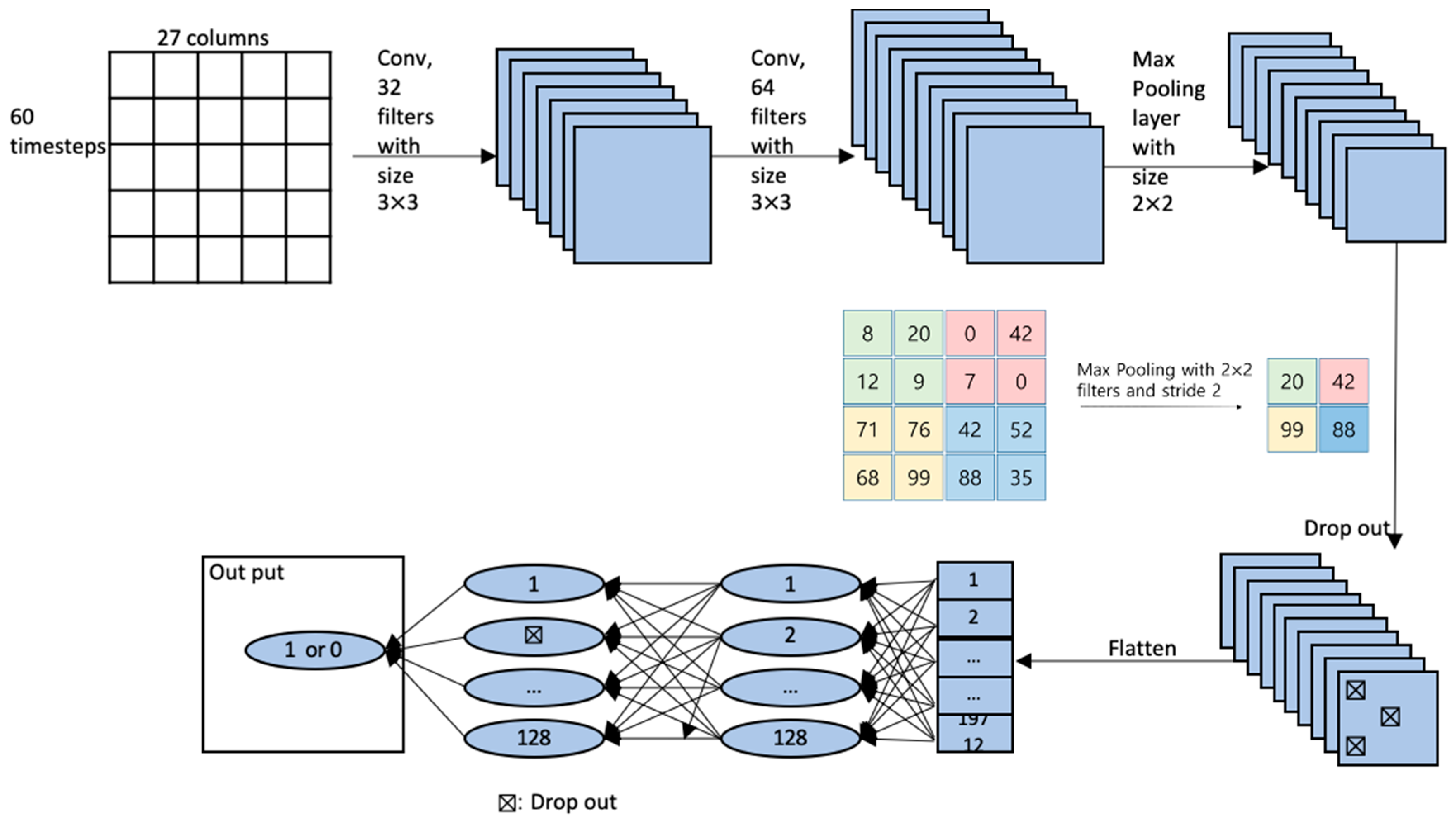
| Layer Type | Input Shape | Filter Shape | Activation | Parameters, # |
|---|---|---|---|---|
| Input | (60, 27, 1) | 0 | ||
| Conv2D | (58, 25, 32) | (3, 3) | Relu | 320 |
| Conv2D | (56, 23, 64) | (3, 3) | Relu | 18,496 |
| MaxPooling2D | (28, 11, 64) | (2, 2) | 0 | |
| Dropout | (28, 11, 64) | 0 | ||
| Flatten | (19712) | 0 | ||
| dense | (128) | Relu | 2,523,264 | |
| Dropout | (128) | 0 | ||
| dense | (1) | sigmoid | 129 |
| Feature Set | Performance Metrics | Random Forest | Xgboost | CNN | DNN | |
|---|---|---|---|---|---|---|
| Vital records | Accuracy | 70.32 | 64.15 | 72.24 | 63.25 | |
| Hypotension | Precision | 69.97 | 65.92 | 72.1 | 64.2 | |
| Recall | 78.28 | 69.15 | 79.04 | 72.12 | ||
| Vital records + EHR | Accuracy | 70.26 | 64.32 | 72.63 | 63.4 | |
| Hypotension | Precision | 69.84 | 66.14 | 72.69 | 64.38 | |
| Recall | 78.37 | 68.99 | 79.33 | 71.99 | ||
| Vital records + EHR + Vasoactive drug | Accuracy | 70.28 | 64.6 | 71.87 | 63.22 | |
| Hypotension | Precision | 69.82 | 66.5 | 72.92 | 64.32 | |
| Recall | 78.35 | 69.05 | 76.37 | 71.95 | ||
| Random Forest | Xgboost | CNN | DNN | ||
|---|---|---|---|---|---|
| All features (97) | Accuracy | 70.76 | 65.15 | 65.33 | 69.03 |
| Precision | 72.16 | 67.37 | 68.29 | 70.78 | |
| Recall | 74.72 | 68.61 | 68.54 | 72.79 | |
| Feature set 1 | Accuracy | 65.26 | 61.75 | 60.34 | 63.03 |
| Precision | 67.02 | 64.81 | 63.79 | 65.57 | |
| Recall | 70.88 | 63.93 | 66.76 | 67.22 | |
| Feature set 2 | Accuracy | 74.89 | 69.84 | 67.95 | 73.85 |
| Precision | 75.8 | 71.5 | 70.69 | 73.72 | |
| Recall | 78.43 | 73.17 | 71.78 | 79.93 | |
| Feature set 3 | Accuracy | 73.06 | 68.28 | 68.95 | 73.84 |
| Precision | 74.59 | 70.19 | 74.11 | 75.73 | |
| Recall | 75.97 | 71.35 | 66.97 | 75.88 | |
| 3 Min | 2 Min | 1 Min | ||
|---|---|---|---|---|
| Vital records + HER with CNN | Accuracy | 72.63 | 70.37 | 70.39 |
| Precision | 72.69 | 71.06 | 71.53 | |
| Recall | 79.33 | 75.64 | 74.64 | |
| Feature set 2 with RF | Accuracy | 74.89 | 71.45 | 74.42 |
| Precision | 75.8 | 72.16 | 72.66 | |
| Recall | 78.43 | 76.26 | 75.17 | |
© 2020 by the authors. Licensee MDPI, Basel, Switzerland. This article is an open access article distributed under the terms and conditions of the Creative Commons Attribution (CC BY) license (http://creativecommons.org/licenses/by/4.0/).
Share and Cite
Lee, J.; Woo, J.; Kang, A.R.; Jeong, Y.-S.; Jung, W.; Lee, M.; Kim, S.H. Comparative Analysis on Machine Learning and Deep Learning to Predict Post-Induction Hypotension. Sensors 2020, 20, 4575. https://0-doi-org.brum.beds.ac.uk/10.3390/s20164575
Lee J, Woo J, Kang AR, Jeong Y-S, Jung W, Lee M, Kim SH. Comparative Analysis on Machine Learning and Deep Learning to Predict Post-Induction Hypotension. Sensors. 2020; 20(16):4575. https://0-doi-org.brum.beds.ac.uk/10.3390/s20164575
Chicago/Turabian StyleLee, Jihyun, Jiyoung Woo, Ah Reum Kang, Young-Seob Jeong, Woohyun Jung, Misoon Lee, and Sang Hyun Kim. 2020. "Comparative Analysis on Machine Learning and Deep Learning to Predict Post-Induction Hypotension" Sensors 20, no. 16: 4575. https://0-doi-org.brum.beds.ac.uk/10.3390/s20164575