An Energy-Efficient Unselfish Spectrum Leasing Scheme for Cognitive Radio Networks


Department of Electrical, Electronic, and Information Engineering “Guglielmo Marconi” (DEI), CNIT, University of Bologna, 40126 Bologna, Italy
*
Author to whom correspondence should be addressed.
Sensors 2020, 20(21), 6161; https://0-doi-org.brum.beds.ac.uk/10.3390/s20216161
Submission received: 1 October 2020
/
Revised: 23 October 2020
/
Accepted: 26 October 2020
/
Published: 29 October 2020
(This article belongs to the Special Issue Advances in Cognitive Radio Networks)
Abstract
:Cooperative Communications in Cognitive Radio (CR) have been introduced as an essential and efficient technique to improve the transmission performance of primary users and offer transmission opportunities for secondary users. In a typical multiuser Cooperative Communication in CR, each primary user can choose one secondary user as a relay node. To encourage the cooperative behavior of the secondary users, primary users lease a fraction of their allocated spectrum to the relay secondary users to transmit their data packets. In this work, a novel unselfish spectrum leasing scheme in CR networks is proposed that offers an energy-efficient solution minimizing the environmental impact of our network. A network management architecture is introduced, and resource allocation is proposed as a constrained sum energy efficiency maximization problem. The optimization problem is formulated and solved using non-linear programming methods and based on a modified Kuhn-Munkres bipartite matching algorithm. System simulations demonstrate an increment in the energy efficiency of the primary users’ network compared with previously proposed algorithms.
1. Introduction
The exponential growth of wireless services in the last decades has called for additional spectrum to accommodate the ever-increasing traffic flow [1]. Besides, the current static spectrum policy, used by most countries in the world, has almost resulted in licensed spectrum exhaustion of some frequency bands [2]. On the contrary, recent spectrum utilization measurements have shown that the available spectrum opportunities are severely underutilized [3]. Cognitive radio (CR), with its ability to sense available frequency bands and adaptively adjust transmission frequency, has attracted considerable attention as one of the most promising solutions to spectrum underutilization [4,5,6,7]. Traditionally in CR networks (CRNs), there two categories of users, namely, primary users (PUs) and secondary users (SUs). PUs are licensed users, and they have the exclusive right to use their respective channels, while SUs are unlicensed, and they wish to use the underutilized channels [8]. To pay off the use of a licensed band, cooperative CRNs (CCRNs) have been proposed in which SUs act as relays to provide a better transmission performance to the PUs [9,10,11].
Extensive research has been conducted regarding spectrum leasing in CCRN. To address the challenges several approaches have been adopted. The game-theoretical approaches, such as Stackelberg game [12], are used to achieve the equilibrium state (e.g., Nash Equilibrium [13,14]) and involves PUs and SUs as players of the game. In Reference [15], a scenario, in which PUs compete for cooperation with available SUs under shared constraint set by SU’s requirements, is modeled as a generalized Nash Equilibrium. The authors of Reference [16], propose a noncooperative game to find the optimal power of SUs consumed in a scenario where SUs are used as relays in cooperation to aid PUs’ transmission. In Reference [17], a spectrum leasing technique to improve the spectral utility of the PUs has been proposed. Nash bargaining is used to determine the optimal division of temporal resources between relaying and reimbursement. In Reference [18], a novel approach is presented in which the spectrum leasing problem is formulated as a Stackelberg game, while the relay selection is solved by the Hungarian method. The authors of Reference [19], derive a cooperative game to find the optimal spectrum leasing time and allocated power of SUs.
Another popular approach is convex optimization. An adaptive spectrum leasing scheme is proposed in Reference [20] to improve the overall network throughput. The authors of Reference [21], present a spectrum leasing scheme for an overlay CRN in which PUs’ transmission is assisted by a cognitive multi-hop multi-branch network. The branch selection and spectrum allocation are jointly optimized such that the sum-rate of the SUs is maximized. A multi-objective optimization framework to incorporate average sum power minimization and the leased time minimization is proposed in Reference [22]. In Reference [23], a cooperative sharing model for cognitive wireless powered networks is proposed, to accomplish PU’s transmission early and vacate opportunity for SU’s transmission. An energy efficiency and spectral efficiency trade-off in an energy harvesting cooperative CRN is addressed in Reference [24]. The objective is to maximize energy and spectral efficiency via joint optimization of spectrum sensing time and self as well as cooperative transmission gains.
Different other approaches have been chosen to address the challenges of spectrum leasing in CCRN. In Reference [25], an opportunistic relaying based spectrum leasing is presented in which PUs lease their frequency band to the SUs and, at the same time, the primary network benefits in terms of outage probability. A cooperative relaying scheme is investigated in Reference [26], where one of the inactive SUs is used as a relay for the PUs. By adopting an aspiration level to model SUs behavior, the SUs’ strategy dynamics is formulated as a discrete-time Markov chain [27].
However, the majority of the research works regarding CRNs, are considered mostly PU-centered, with PUs that decide if and when to exploit SUs as relays based on certain conditions that can improve PUs’ transmission. This approach cannot guarantee full cooperation between PUs and SUs because will be dominated by the selfish behavior of PUs. In addition, networks are required nowadays to be more efficient not only in terms of spectrum use but also in terms of optimal power while guaranteeing a satisfying level of quality of service (QoS). In References [15,25,26], a scenario where a single pair of PUs or SUs is considered. Single user transmissions in CCRN compared to multiuser ones, can result incomplete because a full description of the efficiency of a cell cannot be given. It is proven that the rising number of users in a CCRN can significantly affect the overall performance of the network. Furthermore, spectrum leasing schemes in which PUs or SUs are assumed to have fixed transmission power like in Reference [18], cannot fully exploit the possibility of a more energy efficient network. Besides, energy-efficient systems are required not only from an engineering point of view but also to decrease the environmental impact through networks with a low carbon footprint [28].
Motivated by the aforementioned observations, we aim at jointly minimize the overall power consumption for energy-efficient communication in multiuser CRN. In addition, to provide improved cooperation between PUs and SUs and to secure an unselfish behavior of each user, we propose a resource management network architecture for a considered cell. This architecture, composed of various entities, will be responsible for making decisions regarding the usage of relay and for applying the optimal strategy to achieve the maximum energy efficiency of the cell. Our proposed CRN consists of multiple PUs and multiple SUs in which SUs are used as relays to enhance the PUs’ transmission performance and, in return, PUs lease a fraction of their bandwidth to the corresponding SUs. We formulate an energy efficiency based resource allocation, power allocation, and relay selection as an optimization problem. Our analysis shows that this problem can be divided into two subproblems: (1) power allocation, (2) transmission mode and relay selection. To solve the power allocation subproblem, we choose the maximization of the sum of energy efficiencies as the optimization target. This method was initially introduced in Reference [29] but due to its sum-of-ratio form can become difficult to solve. The method is further developed in our work by transforming power allocation into a subtractive form optimization problem with methods similar to those used to solve classical fractional programming problems [30,31,32]. Therefore, the optimal powers closed-form expressions can be derived through a two-layer optimization. Furthermore, the transmission mode and relay selection subproblem is solved based on a modified Kuhn-Munkres bipartite matching algorithm. System simulations performed in a referenced multiuser case validate the effectiveness of our approach proven by the proposed algorithm’s convergence and the increment in the efficiency of the PUs’ network performance when channel conditions get worse.
To summarize, the main contributions of the paper are:
- A novel unselfish resource allocation scheme for CRNs. Unlike most of works where PUs decide whether or not to cooperate with SUs, the decisions are made by a centralized approach with the goal of improving the overall energy efficiency of the cell.
- A resource management network architecture responsible for maximizing the energy efficiency of the cell.
- We propose a two-stage three-dimensional matching algorithm to maximize the energy efficiency of the cell, in which the joint optimization problem is decoupled into two subproblems and solved separately in two stages.
The rest of this paper is organized as follows. In Section 2, the architecture and the system model for CCRN are introduced. In Section 3, we formulate the energy efficiency based resource allocation, power allocation, and relay selection as an optimization problem. The non-convex energy efficiency for CCRN optimization problem is formulated and solved via an iterative algorithm in Section 4. Section 5 presents numerical performance results, and finally, conclusions are provided in Section 5.
2. Proposed Architecture and System Model for CCRN
In CCRN, one of the goals is to use the available spectrum resources in an efficient and coordinated way to guarantee a satisfying level of QoS for all users and achieve performance enhancement of the whole network. To this end, in this section, we propose a resource management network architecture consisting of a number of user resource management entities (URMEs), local resource management entities (LRMEs), and one cell resource management entity (CRME), as shown in Figure 1. The main functions of UMREs, LRMEs, and CRME are described as follows.
URME: It is a functional module embedded in each PU and SU, used to store channel state information, device characteristics and service requirements, and so forth. Through contacting associated LRMEs, URMEs send the collected information to the LRMEs and receive the resource allocation strategy accordingly also from CRMEs through LRMEs.
LRME: It is deployed in each primary base station (PBS) or secondary base station (SBS), being responsible for managing local resource status through interacting with the associated URMEs and the CRME. More specifically, receiving the network and service information from URMEs and then forwarding to the CRME, and receiving the resource management strategy from the CRME and forwarding to the URMEs.
CRME: By interacting with the LRME, the CMRE receives the network status, channel state information, and user service requirement information of all the users within the cell; then performs the proposed resource allocation and relay selection algorithm to obtain the optimal strategy for the cell and communicated to the associated LRMEs.
System Model
In this paper, we consider a CCRN consisting of multiple PUs, multiple SUs, one PBS, and one SBS. Assume PUs are allowed to transmit to the PBS simultaneously, by orthogonal frequency division multiple access (OFDMA). Further, assume that PUs may transmit to the PBS in direct transmission mode or one-hop relay transmission mode, while the relay SUs may also transmit their own data packets to the SBS. Figure 1 illustrates the scenario considered in this paper.
To encourage SUs to relay data packets for the PUs, we propose a spectrum leasing scheme where the PUs lease part of their allocated spectrum to relay SUs so that they can transmit their own data to the SBS exploiting the licensed spectrum [33,34,35]. In this paper, we assume that the decode-and-forward (DF) scheme is applied at each relay node [36].
Let M and K denote the number of PUs and the number of SUs, respectively, denote the allocated bandwidth of the mth PU, , where denotes the spectrum fraction of the mth PU for transmitting the data packets of the PU in the relay transmission mode, and as a consequence , , is the remaining spectrum available for the relay SU to transmit its own data to the SBS. To support relay communication, the transmission time slot T is divided into two periods. For the first part, the PUs transmit their data packets to the corresponding relay SUs, then the SUs forward the received data packets to the PBS during the remaining time. Meanwhile, the SUs transmit their own data packets to the SBS for the whole time period. Figure 2 shows the time and spectrum division mode for relay transmission of the mth PU.
We assume, all channels undergo flat Rayleigh fading and log-normal shadowing and we consider that LRMEs know all channel state information. The distance between mth PU and kth SU relay is denoted as . Then the channel power gain is represented as = , where denotes the average channel gain at a reference distance m and this gain depends on carrier frequency, transmitter and receiver antenna gains and propagation characteristics, is the path-loss exponent, is a Rayleigh distributed r.v., and is a log-normal r.v. with shadowing parameter . The same channel model is considered for the other links , representing respectively the channel gains of the links between the mth PU and PBS in direct transmission mode, the kth SU and PBS in relay mode, and the kth SU when transmitting its own data to the SBS on the fraction of bandwidth leased by the mth PU.
In the case of multiple relay SUs being available, the optimal relay selection scheme should be designed. For each PU-SU pair, the transmit power of the PU, and the transmit power of the relay SU, consumed during relay and during its own data transmission , should be designed for performance optimization of the network.
3. Proposed Joint Resource Allocation and Relay Selection Scheme
In the following subsections, we formulate an optimization problem, and we present a new solution to the energy efficiency based resource allocation, power allocation, and relay selection.
3.1. Energy Efficiency of PUs
The energy efficiency of all the PUs can be expressed as
where denotes the energy efficiency of the mth PU. As PUs may choose direct transmission or cooperative transmission through a relay SU for information transmission to the PBS, the energy efficiency of the mth PU can be calculated as
where is the energy efficiency of the mth PU when using direct mode, while denotes the transmission indicator of the mth PU for the direct mode. More specifically, if , the mth PU uses direct transmission mode, while for , the PU exploits SU relay assisted transmission. The term denotes the energy efficiency of the mth PU when using the kth SU as relay node for cooperative transmission mode, while is the corresponding transmission and relay selection variable, that is, indicates that the mth PU uses the kth SU as relay node for cooperative transmission, and , otherwise. Note that and are mutually exclusive. In the following subsections, we derive the expression of and , respectively.
3.1.1. Direct Mode
The energy efficiency of the mth PU in direct mode, that is, can be calculated as
where is the power consumed by the mth PU when transmitting in direct mode, denotes the circuit power consumption of the mth PU, which is assumed to be a constant for all the PUs in this paper, and denotes the data rate achieved by the mth PU in direct mode, which can be expressed as
where is the noise power of the link between the mth PU and the PBS. Without loss of generality, the noise power of all the transmission links are assumed to be the same in this paper.
3.1.2. Relay Mode
The energy efficiency of the mth PU when using the kth SU as relay node for cooperative transmission, denoted by , can be expressed as
The denominator is the power consumption of the mth PU when using the kth SU as a relay node and can be calculated as
where denotes the circuit power consumption of the SU which is assumed to be a constant for all the SUs. The numerator represents the data rate of the mth PU when using the kth SU as relay node for cooperative transmission. can be expressed as
where and are, respectively, the data rate of the link from the mth PU to the kth SU
and that from the kth SU to the PBS when the kth SU is chosen as the relay node of the mth PU
3.2. Energy Efficiency of SUs
The energy efficiency of all the SUs in the CCRN, denoted by , can be calculated as
where is the energy efficiency of the kth SU when transmitting its own data on the subchannel leased by the mth PU, which can be calculated as
where denote the data rate of the kth SU when transmitting its own data on the subchannel leased by the mth PU
4. Energy Efficiency for CCRN Problem Formulation and Solution
The total energy efficiency of the PUs and the SUs can be formulated as:
In the following, we propose a joint resource allocation, power allocation, and relay selection strategy to maximize the total energy efficiency (13).
4.1. Optimization Problem Formulation
The energy efficiency based power allocation, transmission mode and relay selection scheme can be obtained by solving the following optimization problem:
C1 represents the transmission mode indicator constraint since it is assumed that every PU can only choose direct transmission mode or relay transmission mode. Similarly, C2 specifies the relay mode indicator constraint as it is assumed that every PU can choose only one SU as its relay node and each SU can only forward packets for one PU. C3, C4 and C5 denote the maximum power constraint where and denote respectively the maximum transmit power of the mth PU and the kth SU. C6-C9 represent the minimum data rate constraints where and denote respectively the minimum required data rate of the mth PU and the kth SU.
The optimization problem in (14) can be classified as a nonlinear binary fractional program and therefore difficult to solve using traditional optimization methods [31]. From the optimization constraints C3–C9 given in (14), it can be shown that such an optimization problem can be transformed equivalently into two subproblems: (1) power allocation, (2) transmission mode and relay selection. The solution for each subproblem is presented in the following subsections.
4.2. Power Allocation Subproblem
Assuming that the mth PU selects direct transmission mode, that is, , the energy efficient optimal power allocation problem can be formulated as:
For the relay transmission mode, when the mth PU selects the kth SU as its relay node, that is, , the energy efficiency of the PU-SU pair can be expressed as
Therefore, the optimal power allocation problem for the mth PU and the kth SU can be formulated as:
4.2.1. Equivalent Problem Transformation
In order to solve the optimization problem in (17), we exploit the fractional programming approach [37]. As we mentioned earlier, we are considering DF at the relay node. In case , our optimization problem becomes:
To proceed, we rewrite the problem in (18) into an equivalent form [38]:
where C7 and C8 denote the energy efficiency constraints.
Theorem 1.
If the set () is the solution for (19), then there exist ν and κ such that () satisfies that Karush-Kuhn-Tucker (KKT) conditions for , , , of the following problem [39]
where . Also the set of solutions satisfies a system of equations for , , , and , with
Proof for Theorem 1 is provided in Appendix A.
In Theorem 1 we proved that by satisfying the system of equations in (21) among the solutions of (20), the optimization problem in (18) can be solved. It shows as well that for an optimization problem with an objective function in fractional form, there exists an equivalent in subtractive form, that is, in our case. As a result, we use the equivalent objective function for the rest of the paper.
4.2.2. Energy Efficiency Maximization
In this section we present an iterative algorithm in order to find solutions for the problem in (20). After transforming our problem (18) into (20), it can be easily proven that the tranformed problem is convex and can be solved using the Lagrange dual method [40,41]. Thus, by relaxing the constraints the Lagrange function can be represented as
where and represent the Lagrange multipliers associated with power constraints and minimum data rate requirements, respectively. The corresponding Lagrange dual method can be expressed as follows:
The above dual problem can be solved by optimizing the transmit power for a fixed set of Lagrange multipliers, and updating the Lagrange multipliers iteratively as well as our parameters . For a given set of Lagrange multipliers , the locally optimal transmit powers can be obtained through calculating the derivative of over the transmit powers and setting it to zero thus obtaining
where .
In case , a similar approach can be followed, leading to the optimization problem:
By applying to (28) the same transformation explained in Theorem 1 and applying Lagrange dual method to the transformed problem, we are able to calculate the transmit powers:
Based on these solutions, we propose a two-layer optimization algorithm. In the inner layer the Lagrange multipliers in (24)–(26) and (28)–(30) can be updated through using the subgradient method [42], that is,
where denotes the learning rate.
In the outer layer the parameters can be updated using Newton-Raphson method [43], that is,
where denotes the learning rate and . Detailed steps of our algorithm are shown in Algorithm 1.
| Algorithm 1. Power Allocation Optimization | |||||||||
| 1: | Set tollerance and maximum number of iterations | ||||||||
| Let , choose , | |||||||||
| Choose arbitrarily , , such that satisfies | |||||||||
| power constraints | |||||||||
| Calculate , and | |||||||||
| if | |||||||||
| then | |||||||||
| else | |||||||||
| end | |||||||||
| Let | |||||||||
| Initialize the Lagrange multipliers | |||||||||
| 2: | if | ||||||||
| update and with (24) and (25) and | |||||||||
| obtain and | |||||||||
| else | |||||||||
| update and with (28) and (29) and | |||||||||
| obtain and | |||||||||
| end | |||||||||
| Update with (26) and obtain | |||||||||
| 3: | Update the Lagrange multipliers using (31)–(36) | ||||||||
| 4: | Compute with , and | ||||||||
| if | |||||||||
| , , | |||||||||
| exit program (convergence reached) | |||||||||
| else | |||||||||
| , , | |||||||||
| = | |||||||||
| update using (37)–(40) | |||||||||
| Update | |||||||||
| end | |||||||||
| go to step 2 unless n reached | |||||||||
For the problem in (15), a similar approach can be followed. By transforming it using Theorem 1 and applying the Lagrange dual method, the optimal transmit power for the direct mode can be obtained.
4.3. Transmission Mode and Relay Selection Subproblem
Given the optimal transmit power of the PUs and the SUs, the total energy efficiency of the network can be calculated as:
The transmission mode and relay selection subproblem can be formulated as:
which is a linear binary optimization problem, that can be solved using graph-based optimization method [44]. To implement such optimization problem, we construct two tables: Table 1a, whose columns contain the maximum energy efficiency when the mth PU chooses direct transmission mode; Table 1b, which contain the optimal energy efficiency when the mth PU chooses the kth SU as a relay node for cooperation mode.
It can be seen that the optimal transmission mode and relay selection solution of (42) is equivalent to finding the maximum sum of the energy efficiency elements which are chosen from various rows and columns, except for the direct mode. From (42), we can see that when the energy efficiency of the cell where only direct transmission is available is larger than all the energy efficiency of a cell where relay transmission is adopted, the PU should choose the direct mode. Hence, to solve the optimization problem formulated in (42), for the mth row, , we first compare the element in direct mode with the other elements in the same row number in Table 1b; if the energy efficiency of the PU obtained in direct mode is the largest, then we set , and delete the corresponding row in Table 1b. For the remaining, we can solve the optimal relay selection subproblem for cooperation transmission mode.
Given the constraints on both PUs and SUs, the optimal relay selection subproblem can be described as a bipartite graph, and the problem of finding the optimal relay can be regarded as an optimal matching algorithm in the bipartite graph that can be solved by a modified Kuhn-Munkres (K-M) algorithm [45,46]. A brief description of this algorithm and of its complexity is presented in Appendix B.
Based on the optimal relay selection results, we obtain the corresponding energy efficiency for cooperative mode, which is compared with that obtained from the direct mode for each PU. If the latter is larger, we set in direct mode the corresponding PU and rerun the K-M algorithm until the optimal energy efficiency obtained for cooperative mode is larger than that from the direct mode for all the PUs. In Algorithm 2, we present a brief description of the algorithm.
| Algorithm 2. Transmission Mode and Relay Selection Optimization | |||||||||
| 1: | Solving optimal power allocation subproblem | ||||||||
| to obtain and , construct Table 1 | |||||||||
| 2: | for the mth PU | ||||||||
| if , | |||||||||
| then | |||||||||
| set | |||||||||
| delete the mth row in Table 1b | |||||||||
| end | |||||||||
| end | |||||||||
| Table 1b is updated | |||||||||
| 3: | repeat | ||||||||
| 4: | Apply K-M algorithm on Table 1b to find | ||||||||
| optimal relay node obtaining | |||||||||
| 5: | if | ||||||||
| set | |||||||||
| set | |||||||||
| Update Table 1b removing the mth row | |||||||||
| end | |||||||||
| 6: | until,∀ PU in Table 1b. | ||||||||
5. Results
In this section, we evaluate the system performance and effectiveness of the proposed solution throughout Monte Carlo simulations. A single PUs’ cell of m radius is considered (see Figure 1), and a summary of the scenario parameters are shown in Table 2. Results are obtained averaging over 5000 independent configuration snapshots, each one with different PUs’ and SUs’ positions within the cell (PUs and SUs are uniformly distributed within the area), and independent realizations of shadowing and fading. Regarding the time slot subdivision between PU and SU, we initially assume , which is the choice maximizing energy efficiency, as shown in Section 5.6.
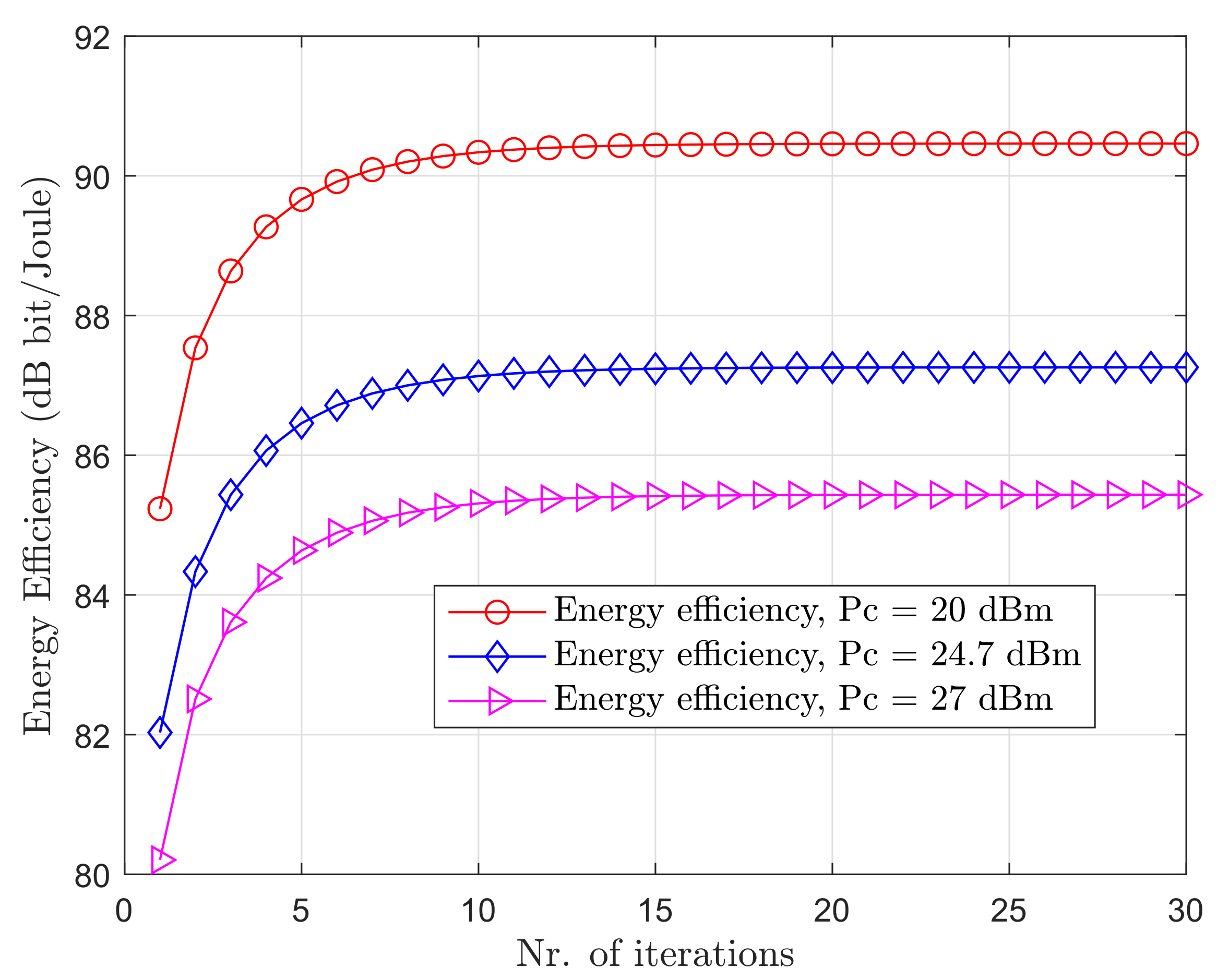
5.1. Convergence of the Iterative Algorithm
In Figure 3, we show the energy efficiency in deciBel, that is, , for different values of PUs’ and SUs’ circuit power, , as a function of the number of iterations, to illustrate the convergence of the proposed algorithm. It can be seen that the iterative algorithm generates a nondecreasing sequence and converges to a stable point within 15 iterations. In addition, we can observe the effect of to energy efficiency. As expected, the energy efficiency decreases with the increase of .
5.2. Energy Efficiency Versus Maximum Transmit Power
In Figure 4, the average energy efficiency varying the maximum transmit power, , is presented. The number of PUs and SUs is chosen randomly at every adaptation with a maximum number of 10 PUs and 10 SUs. From the figure, it can be observed that the energy efficiency increases with an increase of up to approximately W, beyond which the energy efficiency saturates. Besides, we compare the performance of our solution with three different algorithms:
- A random choice algorithm in which PUs choose cooperative relays randomly.
- A non-cooperative approach in which a similar system model is considered but PUs choose relays to increase their own energy efficiency, instead of maximizing the total energy efficiency of the system.
- A system in which there are only PUs, and therefore only direct transmission is possible.
As can be observed, the proposed algorithm outperforms the other three solutions. In addition, compared to a system where only PUs are present, we can show that with our approach having the same available spectrum, higher energy efficiency can be achieved, and also more users are able to use the resources available.
5.3. Energy Efficiency Versus Number of Pus
Figure 5 illustrates the effect that an increasing number of PUs have on energy efficiency when the number of SUs is set to 10. When the number of PUs is smaller than the number of SUs, we can observe a higher energy efficiency achieved. However, increasing the number of PUs, the energy efficiency decreases because of the increased contention of PUs to choose the most convenient cooperative relay. When the number of PUs becomes larger than the number of SUs, the decline of the curve becomes sharper. This comes from the fact that not every PU can choose a cooperative relay and is bounded to perform a direct transmission. As we have shown before, the energy efficiency based only on direct transmission is lower than the one based on the cooperative relay.
5.4. Energy Efficiency Versus Path Loss Exponent
In Figure 6, the average energy efficiency varying the path-loss exponent, , is presented. With the increase of , the energy efficiency decreases; this is due to the increased attenuation, which reflects in a lower data rate. Also, it can be seen that our algorithm outperforms the energy efficiency obtained from the scheme proposed in Reference [18], in which only PUs’ power is optimized, the non-cooperative approach, as well as a system where only PUs are present. In harsh propagation environments with , the energy efficiency of the proposed algorithm outperforms the direct transmission scenario by approximately 110% and the proposed scheme in Reference [18] by 10%.
5.5. Energy Efficiency Versus Shadowing Standard Deviation
In Figure 7, we illustrate the average energy efficiency varying the shadowing standard deviation. As can be seen, also considering the previous figure, the proposed algorithm is more robust to shadowing and attenuation hence offers better performance in harsh propagation environments. The proposed scheme outperforms the direct transmission scenario by 72% and the proposed scheme in Reference [18] by nearly 20%.
5.6. Energy Efficiency Versus Time Slot Division
In Figure 8, the average energy efficiency varying the time slot division chosen in the two relay transmission links is illustrated. As we notice in the figure, when both links have the same duration, we can achieve the highest value of energy efficiency. In addition, it can be observed that the variation between the maximum, for , and minimum value, for , of energy efficiency is not very high. This fact confirms the robustness of the proposed algorithm to the choice of the time slot division in the relay transmission.
6. Conclusions
In this paper, a novel energy-efficient architecture for CRN is proposed where each PU can choose one SU as a relay node. To encourage the cooperative behavior of the SUs, PUs lease a fraction of their allocated spectrum to the relay SUs to transmit their data. We proposed a centralized resource management network architecture to achieve a performance enhancement of the network. The resource allocation problem is formulated as a constrained sum energy efficiency maximization problem. Our analysis shows that this problem can be divided into two subproblems: (1) power allocation, (2) transmission mode and relay selection. To tackle the sum-of-ratio form of the power allocation subproblem, we transform it into a subtractive form optimization problem, and then closed-form optimal powers are calculated through a two-layer optimization. A modified K-M algorithm bipartite matching algorithm is used to solve the transmission mode and relay selection subproblem. System simulations performed in a typical multiuser case show that the proposed algorithm converges to the solution within a small number of iterations. In addition, simulations show an increment in the energy efficiency of the PUs network performance compared to previously proposed algorithms when channel conditions get worse. In addition our proposed algorithm shows a robustness to the choice of the time division in the relay transmission. Furthermore, in the system simulations we illustrated the effect that an increasing number of PUs have on the energy efficiency of the cell. Future work will deal with the use of 3D image-based algorithms to acquire more realistic channel characteristics in more realistic scenarios. In addition, we will consider comparing our algorithm with some existing non-CCRNs-based schemes.
Author Contributions
Conceptualization, D.B.; Investigation, D.B.; Software, D.B.; Supervision, A.G., E.M.V. and V.D.-E.; Validation, D.B., A.G., E.M.V. and V.D.-E.; Visualization, A.G., E.M.V., V.D.-E.; Writing—original draft, D.B.; Writing—review and editing, A.G., E.M.V. and V.D.-E. All authors have read and agreed to the published version of the manuscript.
Funding
This work was supported in part by the Italian Ministry of Education, University and Research (MIUR) under the program “Dipartimenti di Eccellenza (2018–2022)—Precise CPS”, and by the EU COST action CA15104 “Inclusive Radio Communications (IRACON)”.
Conflicts of Interest
The authors declare no conflict of interest.
Appendix A. Proof of Theorem 1
To solve the problem in (19), Lagrange dual method is used [41]. For this purpose, we first need the Lagrange function of this problem. The Lagrangian can be written as:
If the set of solutions () is the solution of the problem in (19), then exist the Lagrange multipliers in order to satisfy the KKT conditions [39] for the problem (19). The conditions are as follows:
Considering that and then from (A3) and (A4) we have
and (A11) and (A12) are equivalent to
The system Equations (A2), (A5)–(A10) are the KKT conditions of the optimization problem in (20) for , , , .
Appendix B. Summary of the Kuhn-Munkres Algorithm
For the sake of completeness, we briefly introduce some definitions and a theorem regarding the K-M algorithm.
Bipartite: A bipartite graph is a graph whose vertices can be divided into two disjoint sets U and V, such that every edge connects a vertex in U to one in V. It can be represented as with E denoting the edges of the graph.
Weighted bipartite: A weighted bipartite is a bipartite in which each edge has a weight factor .
Matching: A matching in a graph is a subset . If H and G share the same vertex set, then H is called a complete matching. The size of a matching is denoted as which equals to the number of edges in H.
Feasible vertex labeling: A feasible vertex labeling in G is a real-valued function l on such that for and ,
Equality subgraph: If l is a feasible labeling, we denote a subgraph of G as which contains a number of edges and the endpoints of these edges. If the edges of meet the condition , then is called the equality subgraph for l.
Theorem A1.
If l is a feasible vertex labeling for G, and H is a complete matching of U to V with , then H is an optimal assignment of U to V.
Appendix B.1. Solving Optimal Relay Selection Problem Based on K-M Algorithm
Applying K-M algorithm to solve the optimal relay selection problem of the PUs, a weighted bipartite graph G with a bipartite division is constructed, where the set of vertices U represents the set of PUs, that is, and the set of vertices V represents the set of SUs, . The weight of the edge in the weighted bipartite graph can be defined as the joint energy efficiency of the mth PU and the kth SU, that is, , and .
The steps of solving the optimal relay selection problem based on K-M algorithm can be described as follows:
- Find initial feasible vertex labeling and determine and choose an arbitrary matching H in .
- If H is a maximum matching for G, then the optimization problem is solved. Otherwise, the label having not being allotted by the distribution H is selected in . Set , and , which denotes the empty set.
- denotes the collection of points which connect with S in . If , go to step (2). Otherwise, . Findand replace existing labeling l with by
The process continues until an equal subgraph consisting a complete match is obtained.
Appendix B.2. Complexity of the K-M Algorithm
Theoretically, the K-M algorithm is guaranteed to reach the global optimal solution [47]. It is the first proved polynomial algorithm and it was observed to be a strongly polynomial by Munkres in Reference [48]. Further, Edmonds and Karp in Reference [49] noticed that it can be modified to running time.
In our case in each of the steps (1) or (2) the algorithm adds one edge to the matching and this happens . In addition, it needs to find the right vertex (if there is one) and improving the labelling takes time to find delta and to update the labelling accordingly. We might have to improve the labelling times until we matching occurs. This makes for a total of . In all, there are iterations each taking work, leading to a total running time of .
References
- Bartoli, G.; Marabissi, D.; Pucci, R.; Ronga, L.S. AI Based Network and Radio Resource Management in 5G HetNets. J. Signal Process. Syst. 2017, 89, 133–143. [Google Scholar] [CrossRef]
- Federal Communications Commission. ET Docket No. 03–322. Notice of Proposed Rule Making and Order. Available online: https://docs.fcc.gov/public/attachments/FCC-03-322A1.pdf (accessed on 28 October 2020).
- Bartoli, G.; Fantacci, R.; Gei, F.; Marabissi, D.; Micciullo, L. Dynamic PSS and commercial networks spectrum sharing in the time domain. Trans. Emerg. Telecommun. Technol. 2016, 28, e3083. [Google Scholar] [CrossRef]
- Mitola, J.; Maguire, G.Q. Cognitive radio: Making software radios more personal. IEEE Pers. Commun. 1999, 6, 13–18. [Google Scholar] [CrossRef] [Green Version]
- Sithamparanathan, K.; Giorgetti, A. Cognitive Radio Techniques: Spectrum Sensing, Interference Mitigation, and Localization; Artech House: Boston, MA, USA, 2012. [Google Scholar]
- Giorgetti, A.; Varrella, M.; Chiani, M. Analysis and performance comparison of different cognitive radio algorithms. In Proceedings of the 2009 Second International Workshop on Cognitive Radio and Advanced Spectrum Management, Aalborg, Denmark, 18–20 May 2009; pp. 127–131, Invited Paper. [Google Scholar]
- Fantacci, R.; Marabissi, D. Cognitive Spectrum Sharing: An Enabling Wireless Communication Technology for a Wide Use of Smart Systems. Future Internet 2016, 8, 23. [Google Scholar] [CrossRef] [Green Version]
- Aqeel, S.; Kok-Lim, Y. Spectrum Leasing in Cognitive Radio Networks: A Survey. Int. J. Distrib. Sens. Netw. 2014, 10, 329235. [Google Scholar]
- Amin, O.; Ikki, S.S.; Uysal, M. On the performance analysis of multi-relay cooperative diversity systems with channel estimation errors. IEEE Trans. Veh. Technol. 2011, 60, 2050–2059. [Google Scholar] [CrossRef]
- Amin, O.; Lampe, L. Opportunistic Energy Efficient Cooperative Communication. IEEE Wirel. Commun. Lett. 2012, 1, 412–415. [Google Scholar] [CrossRef]
- Amin, O.; Ikki, S.S.; Uysal, M. Adaptive bit loading for multi-relay cooperative orthogonal frequency division multiple with imperfect channel estimation. IET Commun. 2012, 6, 1821–1828. [Google Scholar] [CrossRef]
- Nie, P.Y.; Zhang, P. A note on Stackelberg games. In Proceedings of the Chinese Control and Decision Conference, Yantai, China, 2–4 July 2008; pp. 1201–1203. [Google Scholar]
- Scutari, G.; Pang, J. Joint Sensing and Power Allocation in Nonconvex Cognitive Radio Games: Nash Equilibria and Distributed Algorithms. IEEE Trans. Inf. Theory 2013, 59, 4626–4661. [Google Scholar] [CrossRef]
- Xu, H.; Gao, H.; Zhou, C.; Duan, R.; Zhou, X. Resource Allocation in Cognitive Radio Wireless Sensor Networks with Energy Harvesting. Sensors 2019, 19, 5115. [Google Scholar] [CrossRef] [Green Version]
- Elkourdi, T.; Simeone, O. Spectrum Leasing via Cooperation With Multiple Primary Users. IEEE Trans. Veh. Technol. 2012, 61, 820–825. [Google Scholar] [CrossRef]
- Toroujeni, S.M.M.; Sadough, S.M.; Ghorashi, S.A. Spectrum Leasing for OFDM-Based Cognitive Radio Networks. IEEE Trans. Veh. Technol. 2013, 62, 2131–2139. [Google Scholar] [CrossRef]
- Hafeez, M.; Elmirghani, J.M.H. Dynamic Spectrum Leasing for Bi-Directional Communication: Impact of Selfishness. IEEE Trans. Commun. 2016, 64, 2427–2437. [Google Scholar] [CrossRef] [Green Version]
- Tang, Y.; Grace, D.; Wang, L. Spectrum Leasing and Relay Selection in Multiuser Cooperative Cognitive Radio Networks. J. Commun. 2014, 9, 198–207. [Google Scholar] [CrossRef]
- Liu, Z.; Zhao, M.; Xie, Y.; Li, X.; Ma, K. Relay selection and power allocation for spectrum leasing in cooperative cognitive radio networks. In Proceedings of the Chinese Control Conference (CCC), Dalian, China, 26–28 July 2017; pp. 8958–8963. [Google Scholar]
- Zhai, C.; Zhang, W. Adaptive Spectrum Leasing with Secondary User Scheduling in Cognitive Radio Networks. IEEE Trans. Wirel. Commun. 2013, 12, 3388–3398. [Google Scholar] [CrossRef]
- Bastami, A.H.; Kazemi, P. Cognitive Multi-Hop Multi-Branch Relaying: Spectrum Leasing and Optimal Power Allocation. IEEE Trans. Wirel. Commun. 2019, 18, 4075–4088. [Google Scholar] [CrossRef]
- Ma, Y.; Yin, X.; Yang, X.; Liu, Q. Resource allocation for spectrum-leasing based CRN with delay-sensitive traffic. EURASIP J. Wirel. Commun. Netw. 2017, 108. [Google Scholar] [CrossRef] [Green Version]
- Yin, S.; Qu, Z.; Wang, Z.; Li, L. Energy-Efficient Cooperation in Cognitive Wireless Powered Networks. IEEE Commun. Lett. 2017, 21, 128–131. [Google Scholar] [CrossRef]
- Chatterjee, S.; Maity, S.P.; Acharya, T. Energy-Spectrum Efficiency Trade-Off in Energy Harvesting Cooperative Cognitive Radio Networks. IEEE Trans. Cogn. Commun. Netw. 2019, 5, 295–303. [Google Scholar] [CrossRef]
- Kong, H.Y.; Koo, I. Opportunistic relaying based spectrum leasing for cognitive radio networks. J. Commun. Netw. 2011, 13, 50–55. [Google Scholar] [CrossRef]
- Kader, M.F.; Chowdhury, M. Cooperative secondary user selection as a relay for the primary system in underlay cognitive radio networks. In Proceedings of the 15th International Conference on Computer and Information Technology (ICCIT), Chittagong, Bangladesh, 22–24 December 2012; pp. 275–278. [Google Scholar]
- Shao, C.; Roh, H.; Lee, W. Aspiration Level-Based Strategy Dynamics on the Coexistence of Spectrum Cooperation and Leasing. IEEE Commun. Lett. 2014, 18, 70–73. [Google Scholar] [CrossRef]
- Marabissi, D.; Bartoli, G.; Fantacci, R.; Micciullo, L. Energy efficient cooperative multicast beamforming in ultra dense networks. IET Commun. 2017, 12, 573–578. [Google Scholar] [CrossRef]
- Bilibashi, D.; Chai, R. Energy Efficiency Based Resource Allocation Scheme for Cooperative Cognitive Radio Networks. Int. J. Electron. Electr. Eng. 2017, 5, 7–14. [Google Scholar] [CrossRef]
- Jagannathan, R. On some properties of programming problems in parametric form pertaining to fractional programming. Manag. Sci. 1966, 12, 609–615. [Google Scholar] [CrossRef]
- Dinkelbach, W. On nonlinear fractional programming. Manag. Sci. 1967, 13, 492–498. [Google Scholar] [CrossRef]
- Dür, M.; Horst, R.; Thoai, N. Solving sum-of-ratios fractional programs using efficient points. Optimization 2001, 49, 447–466. [Google Scholar] [CrossRef]
- Darsena, D.; Gelli, G.; Melito, F.; Verde, F. Performance Analysis of Amplify-and-Forward Multiple-Relay MIMO Systems with ZF Reception. IEEE Trans. Veh. Technol. 2015, 64, 3274–3280. [Google Scholar] [CrossRef]
- Verde, F.; Scaglione, A.; Darsena, D.; Gelli, G. An Amplify-and-Forward Scheme for Spectrum Sharing in Cognitive Radio Channels. IEEE Trans. Wirel. Commun. 2015, 14, 5629–5642. [Google Scholar] [CrossRef]
- Amin, O.; Uysal, M. Adaptive power loading for multi-relay OFDM Regenerative networks with relay selection. IEEE Trans. Commun. 2012, 60, 614–619. [Google Scholar] [CrossRef]
- Bagheri, S.; Verde, F.; Darsena, D.; Scaglione, A. Randomized Decode-and-Forward Strategies for Two-Way Relay Networks. IEEE Trans. Wirel. Commun. 2011, 12, 4214–4225. [Google Scholar] [CrossRef]
- Bertsekas, D.P. Nonlinear Programming, 2nd ed.; Athena Scientific: Belmont, MA, USA, 1999. [Google Scholar]
- He, S.; Huang, Y.; Yang, L.; Ottersten, B. Coordinated Multicell Multiuser Precoding for Maximizing Weighted Sum Energy Efficiency. IEEE Trans. Signal Process. 2014, 62, 741–751. [Google Scholar] [CrossRef]
- Borwein, J.; Lewis, A. Convex Analysis and Nonlinear Optimization: Theory and Examples; Springer: New York, NY, USA, 2006. [Google Scholar]
- Ng, D.W.K.; Lo, E.S.; Schober, R. Energy-Efficient Resource Allocation in OFDMA Systems with Large Numbers of Base Station Antennas. IEEE Trans. Wirel. Commun. 2012, 11, 3292–3304. [Google Scholar] [CrossRef]
- Boyd, S.; Vandenberghe, L. Convex Optimization; Cambridge University Press: Cambridge, UK, 2004. [Google Scholar]
- Boyd, S.; Mutapcic, A. Subgradient Methods, Notes for EE364; Standford University: Stanford, CA, USA, 2006. [Google Scholar]
- Lee, E.T.; Wang, J.W. Statistical Methods for Survival Data Analyses, 3rd ed.; John Wiley and Sons, Inc.: Hoboken, NJ, USA, 2003; pp. 428–432. [Google Scholar]
- Samanta, S.; Sarkar, B. Isomorphism on generalized fuzzy graphs and image visualizations. Soft Comput. 2020, 24, 14401–14409. [Google Scholar] [CrossRef]
- Kuhn, H. The hungarian method for the assignment problem. Naval Res. Logist. Q. 1955, 2, 83–97. [Google Scholar] [CrossRef] [Green Version]
- Mensah, K.K.; Chai, R.; Bilibashi, D.; Gao, F. Energy efficiency based joint cell selection and power allocation scheme for HetNets. Digit. Commun. Netw. 2016, 2, 184–190. [Google Scholar] [CrossRef]
- Hong, C.; Jingjing, Z.; Chunfeng, C.; Qinyu, C. Solving large-scale assignment problems by Kuhn-Munkres algorithm. In Proceedings of the International Conference on Advances in Mechanical Engineering and Industrial Informatics, Hangzhou, China, 9–10 April 2016. [Google Scholar]
- Bourgeois, F.; Lassalle, J.C. An extension of the munkres algorithm for the assignment problem to rectangular matrices. Commun. ACM 1971, 14, 802–804. [Google Scholar] [CrossRef]
- Edmonds, J.; Karp, R.M. Theoretical improvements in algorithmic efficiency for network flow problems. Commun. ACM 1972, 19, 248–264. [Google Scholar] [CrossRef]
Figure 1.
Proposed architecture and scenario for the cell.

Figure 2.
Bandwidth allocation and time slot division for primary user (PU) and secondary user (SU).
Figure 2.
Bandwidth allocation and time slot division for primary user (PU) and secondary user (SU).

Figure 3.
Energy efficiency versus number of iterations with and , for different circuit power consumption .
Figure 3.
Energy efficiency versus number of iterations with and , for different circuit power consumption .

Figure 4.
Energy efficiency varying the maximum transmit power. Three different algorithms are compared. M and K in this case change randomly from 1 to 10.
Figure 4.
Energy efficiency varying the maximum transmit power. Three different algorithms are compared. M and K in this case change randomly from 1 to 10.

Figure 5.
Energy efficiency varying number of PUs. M varies from 2 to 18 and .

Figure 6.
Energy efficiency increment with respect to direct mode varying the path loss exponent. M and K change randomly from 1 to 15 while = 8dB.
Figure 6.
Energy efficiency increment with respect to direct mode varying the path loss exponent. M and K change randomly from 1 to 15 while = 8dB.

Figure 7.
Energy efficiency increment with respect to direct mode versus shadowing standard deviation. M and K in this case change randomly within 1 and 15 while = 3.
Figure 7.
Energy efficiency increment with respect to direct mode versus shadowing standard deviation. M and K in this case change randomly within 1 and 15 while = 3.

Figure 8.
Energy efficiency versus time slot division in the relay transmission link. The parameters M and K are random variables uniformly distributed from 1 to 10.
Figure 8.
Energy efficiency versus time slot division in the relay transmission link. The parameters M and K are random variables uniformly distributed from 1 to 10.


Table 1.
Tables of direct mode and cooperative mode.
| (a) Direct Mode | (b) Cooperative Mode | ||||
|---|---|---|---|---|---|
| Direct Mode | Coop. with SU | Coop. with SU | ⋯ | Coop. with SU | |
| PU | ⋯ | ||||
| PU | ⋯ | ||||
| ⋯ | ⋯ | ⋯ | |||
| PU | ⋯ | ||||
Table 2.
System parameters.
| Cell radius | m |
| Small scale fading distribution | Rayleigh fading |
| Carrier frequency | GHz |
| Bandwidth | MHz |
| Noise power per link, | dBm |
| Shadowing, | Log-normal with standard deviation of dB |
| Average channel gain at 1 m, | dB |
| Path-loss exponent, | 3 |
| Circuit power per UE (PU or SU), | dBm |
| Maximum transmit power per UE, | dBm |
| Minimum data rate constraint, | Mbit/s |
| Fraction of bandwidth, |
Publisher’s Note: MDPI stays neutral with regard to jurisdictional claims in published maps and institutional affiliations. |
© 2020 by the authors. Licensee MDPI, Basel, Switzerland. This article is an open access article distributed under the terms and conditions of the Creative Commons Attribution (CC BY) license (http://creativecommons.org/licenses/by/4.0/).
Share and Cite
MDPI and ACS Style
Bilibashi, D.; Vitucci, E.M.; Degli-Esposti, V.; Giorgetti, A. An Energy-Efficient Unselfish Spectrum Leasing Scheme for Cognitive Radio Networks. Sensors 2020, 20, 6161. https://0-doi-org.brum.beds.ac.uk/10.3390/s20216161
AMA Style
Bilibashi D, Vitucci EM, Degli-Esposti V, Giorgetti A. An Energy-Efficient Unselfish Spectrum Leasing Scheme for Cognitive Radio Networks. Sensors. 2020; 20(21):6161. https://0-doi-org.brum.beds.ac.uk/10.3390/s20216161
Chicago/Turabian StyleBilibashi, Denis, Enrico M. Vitucci, Vittorio Degli-Esposti, and Andrea Giorgetti. 2020. "An Energy-Efficient Unselfish Spectrum Leasing Scheme for Cognitive Radio Networks" Sensors 20, no. 21: 6161. https://0-doi-org.brum.beds.ac.uk/10.3390/s20216161
Note that from the first issue of 2016, this journal uses article numbers instead of page numbers. See further details here.