SodSAR: A Tower-Based 1–10 GHz SAR System for Snow, Soil and Vegetation Studies

 , , and
Abstract
:1. Introduction
2. SodSAR Description
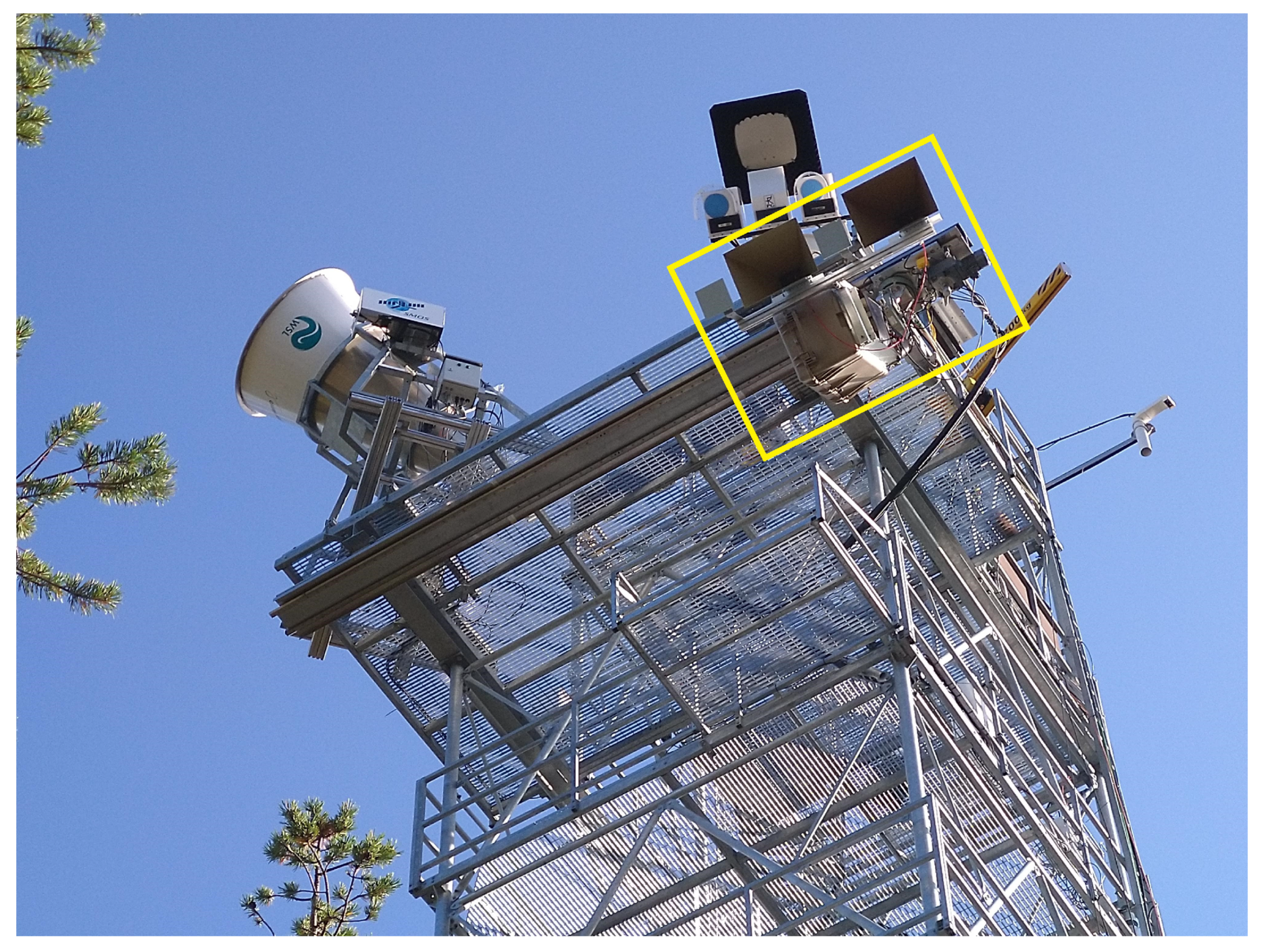
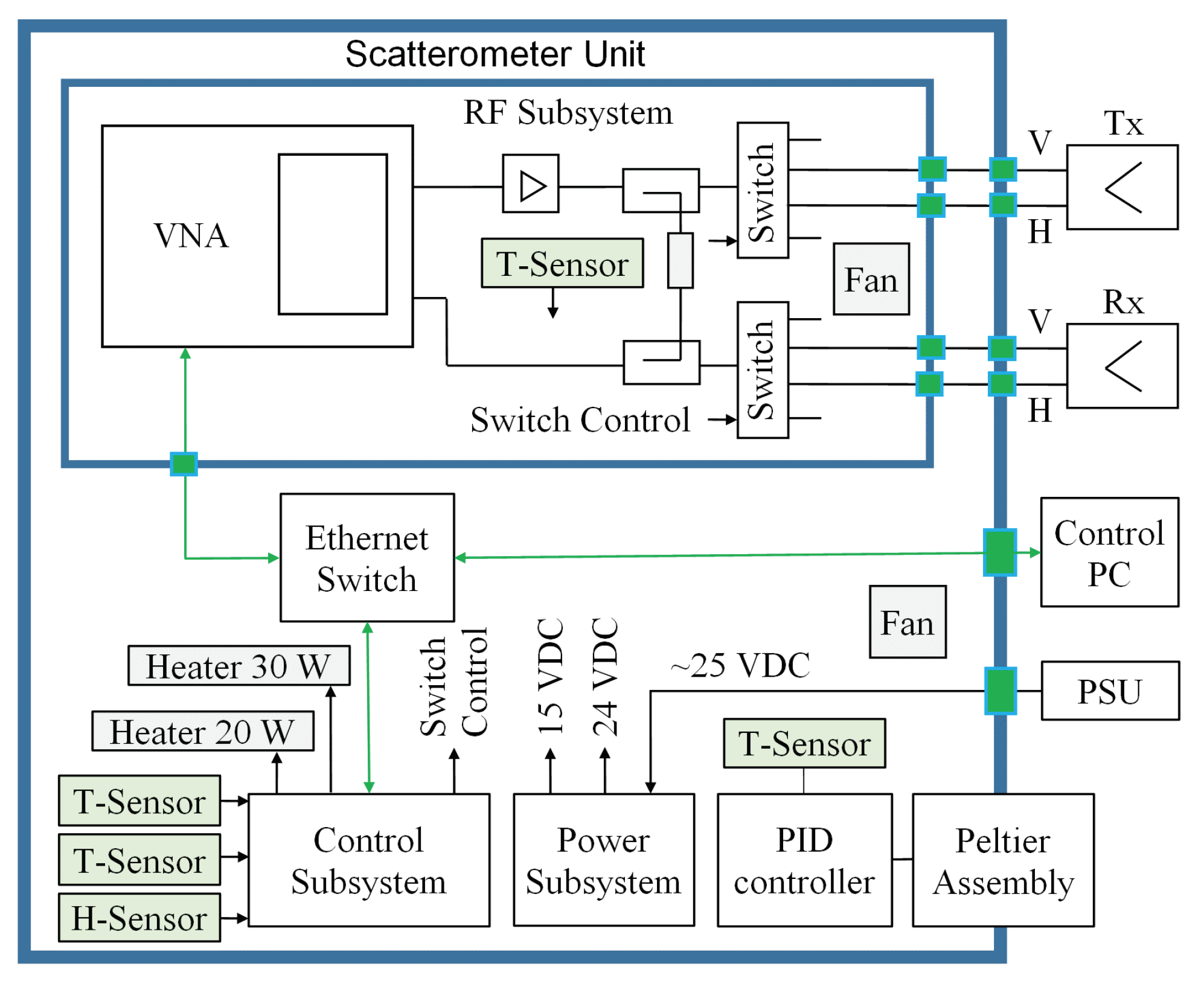
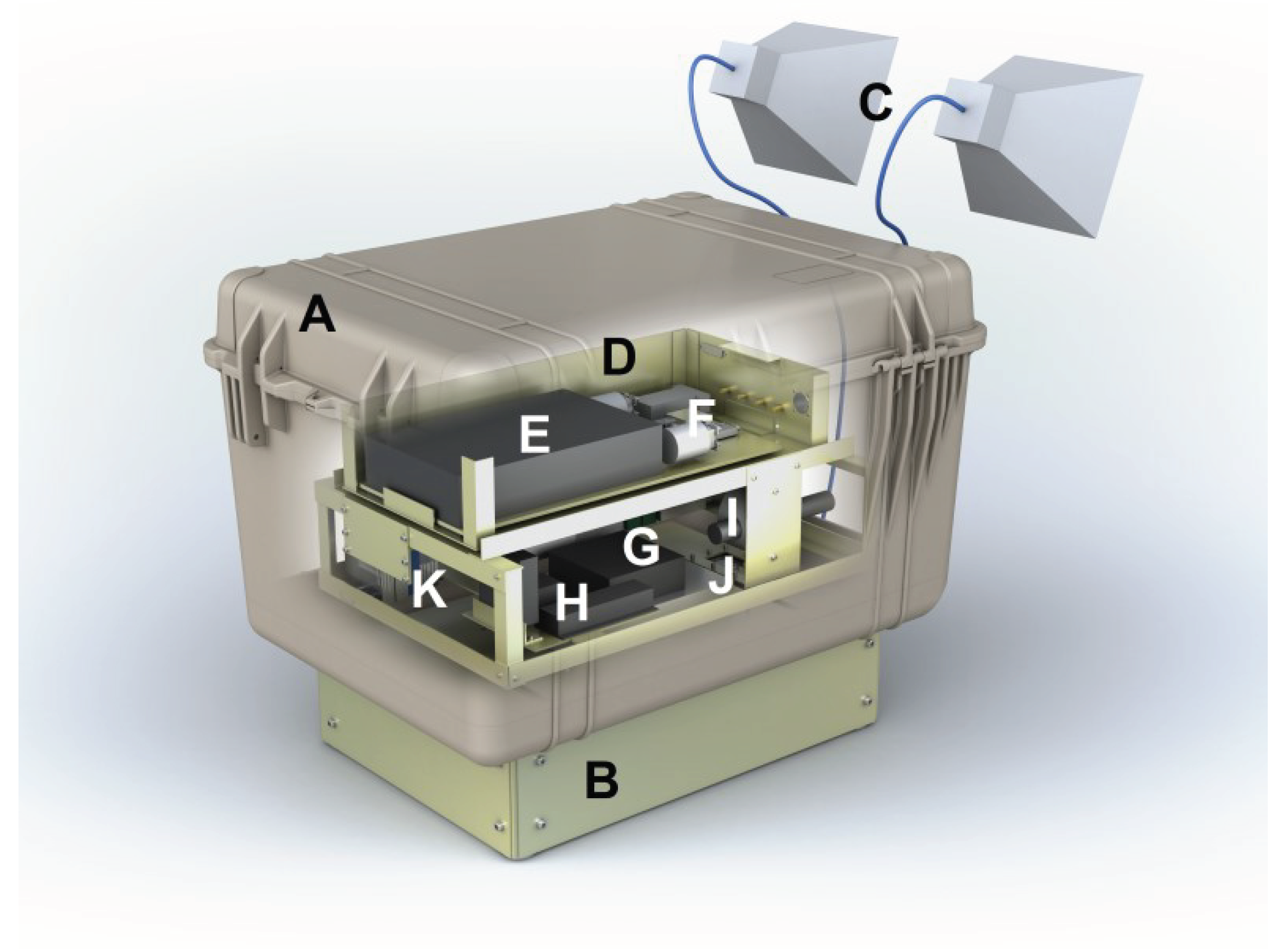
2.1. Description of Scatterometer Unit
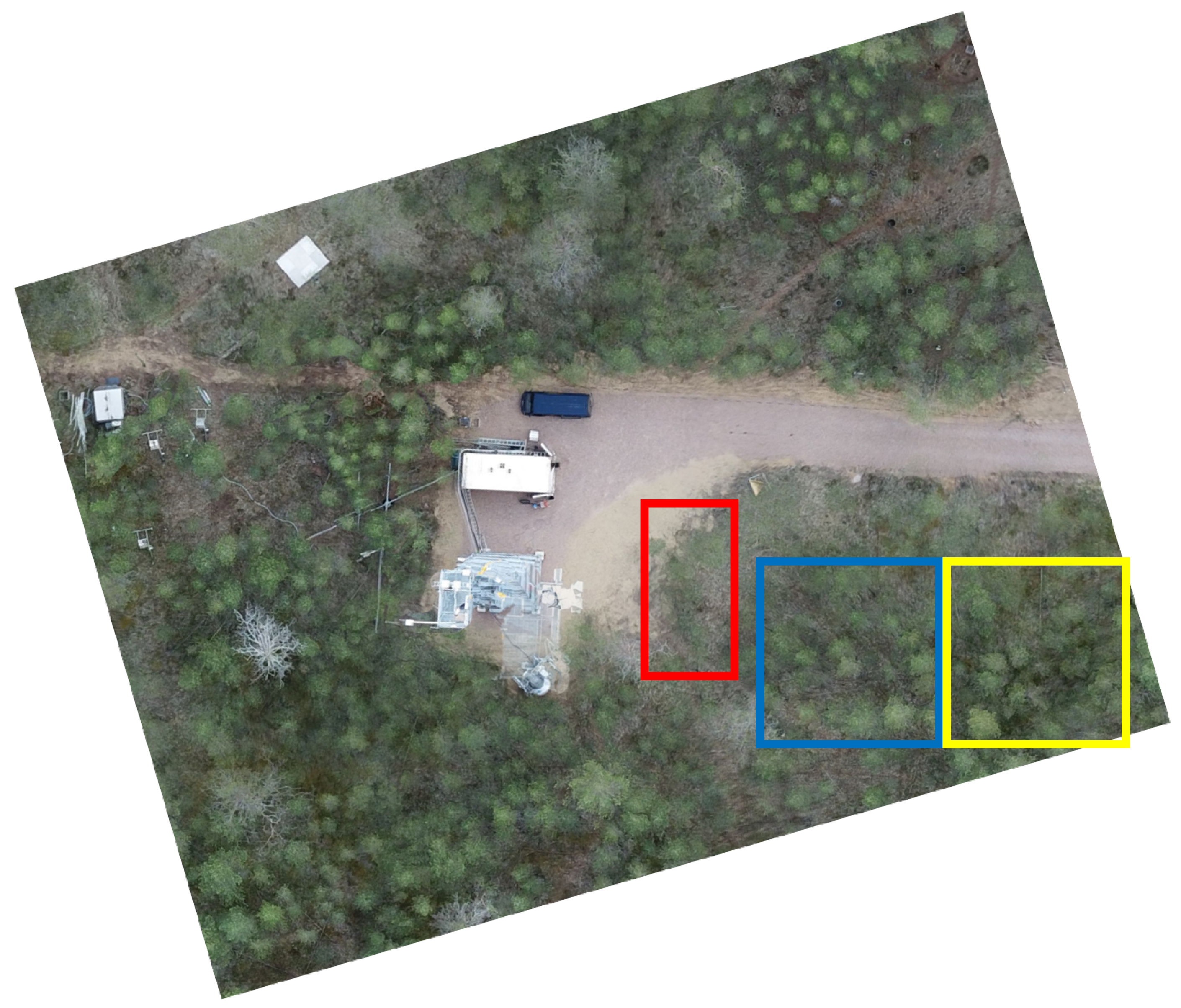
2.2. Installation and Operation
3. SAR Signal Processing
3.1. Sampling Requirements for SAR Operation
3.2. Image Resolution
3.3. SAR Image Reconstruction
4. Radar Calibration and Measurement Stability
4.1. Calibration
4.2. Measurement Stability
5. SodSAR as an InSAR
5.1. Processing
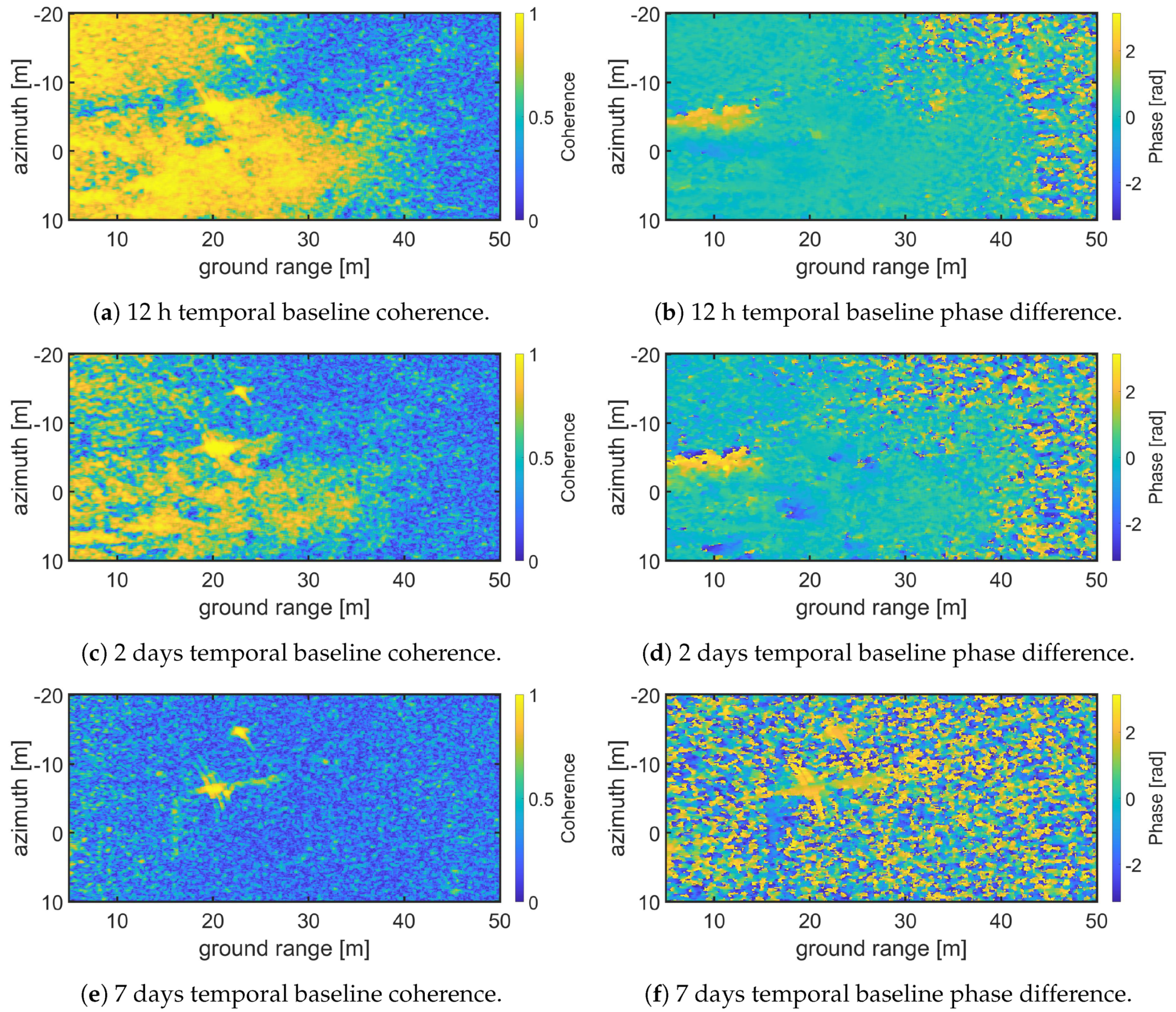
5.2. InSAR Examples
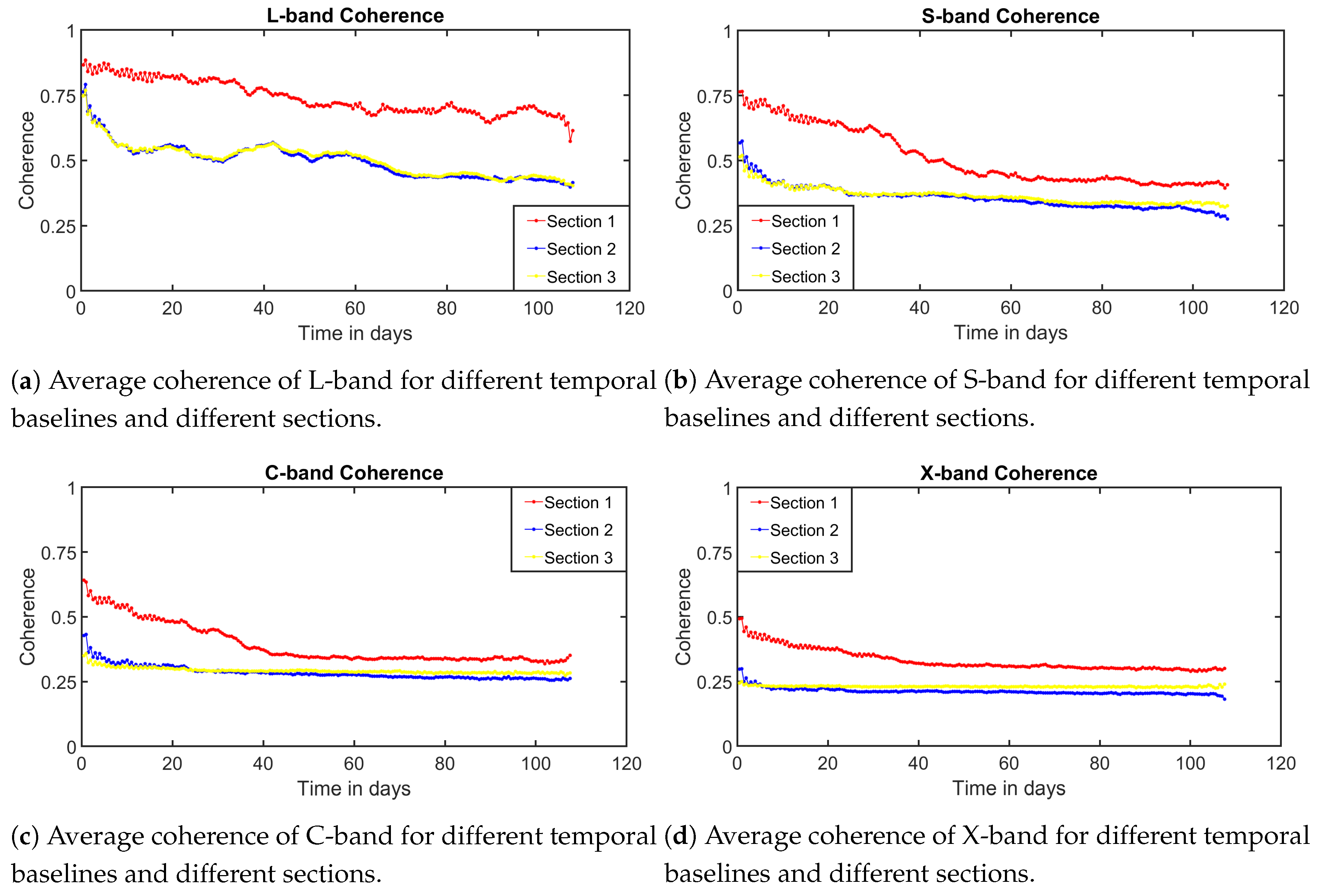
5.3. Temporal Coherence Analysis
6. Potential Applications of SodSAR
7. Conclusions
Author Contributions
Funding
Conflicts of Interest
References
- Evans, D.L.; Alpers, W.; Cazenave, A.; Elachi, C.; Farr, T.; Glackin, D.; Holt, B.; Jones, L.; Liu, W.T.; McCandless, W.; et al. Seasat—A 25-year legacy of success. Remote Sens. Environ. 2005, 94, 384–404. [Google Scholar] [CrossRef]
- Davidson, M.; Snoeij, P.; Attema, E.; Rommen, B.; Floury, N.; Levrini, G.; Duesmann, B. Sentinel-1 Mission Overview. In Proceedings of the 2009 IEEE International Geoscience and Remote Sensing Symposium, Cape Town, South Africa, 12–17 July 2009; Volume 1, pp. 1–4. [Google Scholar] [CrossRef]
- Thompson, A.; Kelly, R.; King, J. Sensitivity of Ku- and X-Band Radar Observations to Seasonal Snow in Ontario, Canada. Can. J. Remote Sens. 2019, 45, 829–846. [Google Scholar] [CrossRef]
- Tan, S.; Chang, W.; Tsang, L.; Lemmetyinen, J.; Proksch, M. Modeling Both Active and Passive Microwave Remote Sensing of Snow Using Dense Media Radiative Transfer (DMRT) Theory With Multiple Scattering and Backscattering Enhancement. IEEE J. Sel. Top. Appl. Earth Obs. Remote Sens. 2015, 8, 4418–4430. [Google Scholar] [CrossRef]
- King, J.; Derksen, C.; Toose, P. Exploring the influence of snow microstructure on dual-frequency radar measurements. In Proceedings of the 2017 IEEE International Geoscience and Remote Sensing Symposium (IGARSS), Fort Worth, TX, USA, 23–28 July 2017; pp. 1355–1358. [Google Scholar] [CrossRef]
- Lemmetyinen, J.; Derksen, C.; Rott, H.; Macelloni, G.; King, J.; Schneebeli, M.; Wiesmann, A.; Leppänen, L.; Kontu, A.; Pulliainen, J. Retrieval of Effective Correlation Length and Snow Water Equivalent from Radar and Passive Microwave Measurements. Remote Sens. 2018, 10, 170. [Google Scholar] [CrossRef] [Green Version]
- Monteith, A.R.; Ulander, L.M.H. Temporal Survey of P- and L-Band Polarimetric Backscatter in Boreal Forests. IEEE J. Sel. Top. Appl. Earth Obs. Remote. Sens. 2018, 11, 3564–3577. [Google Scholar] [CrossRef]
- Zhou, Z.-S.; Boerner, W.; Sato, M. Development of a ground-based polarimetric broadband SAR system for noninvasive ground-truth validation in vegetation monitoring. IEEE Trans. Geosci. Remote Sens. 2004, 42, 1803–1810. [Google Scholar] [CrossRef] [Green Version]
- Gromek, A. High resolution SAR imaging trials using a handheld vector network analyzer. In Proceedings of the 2014 15th International Radar Symposium (IRS), Gdansk, Poland, 16–18 June 2014; pp. 1–4. [Google Scholar]
- Werner, C.; Wiesmann, A.; Strozzi, T.; Schneebeli, M.; Mätzler, C. The SnowScat ground-based polarimetric scatterometer: Calibration and initial measurements from Davos Switzerland. In Proceedings of the 2010 IEEE International Geoscience and Remote Sensing Symposium, Honolulu, HI, USA, 25–30 July 2010; pp. 2363–2366. [Google Scholar]
- Lemmetyinen, J.; Kontu, A.; Leppänen, L.; Vehviläinen, J.; Vehmas, R.; Li, Q.; Rautiainen, K.; Pulliainen, J. Season-Length Observations of Active and Passive Microwave Signatures of Snow Cover in a Boreal Forest Environment. In Proceedings of the IGARSS 2018—2018 IEEE International Geoscience and Remote Sensing Symposium, Valencia, Spain, 22–27 July 2018; pp. 6262–6265. [Google Scholar] [CrossRef]
- Frey, O.; Werner, C.L.; Wiesmann, A. Tomographic profiling of the structure of a snow pack at X-/Ku-Band using SnowScat in SAR mode. In Proceedings of the 2015 European Radar Conference (EuRAD), Paris, France, 9–11 September 2015; pp. 21–24. [Google Scholar] [CrossRef]
- Leinss, S.; Wiesmann, A.; Lemmetyinen, J.; Hajnsek, I. Snow Water Equivalent of Dry Snow Measured by Differential Interferometry. IEEE J. Sel. Top. Appl. Earth Obs. Remote Sens. 2015, 8, 3773–3790. [Google Scholar] [CrossRef] [Green Version]
- Ulander, L.M.H.; Monteith, A.R.; Soja, M.J.; Eriksson, L.E.B. Multiport Vector Network Analyzer Radar for Tomographic Forest Scattering Measurements. IEEE Geosci. Remote Sens. Lett. 2018, 15, 1897–1901. [Google Scholar] [CrossRef]
- Albinet, C.; Borderies, P.; Koleck, T.; Rocca, F.; Tebaldini, S.; Villard, L.; Le Toan, T.; Hamadi, A.; Ho Tong Minh, D. TropiSCAT: A Ground Based Polarimetric Scatterometer Experiment in Tropical Forests. IEEE J. Sel. Top. Appl. Earth Obs. Remote Sens. 2012, 5, 1060–1066. [Google Scholar] [CrossRef]
- El Idrissi Essebtey, S.; Villard, L.; Borderies, P.; Koleck, T.; Monvoisin, J.P.; Burban, B.; Le Toan, T. Temporal Decorrelation of Tropical Dense Forest at C-Band: First Insights From the TropiScat-2 Experiment. IEEE Geosci. Remote Sens. Lett. 2020, 17, 928–932. [Google Scholar] [CrossRef]
- Albinet, C.; Koleck, T.; Le Toan, T.; Borderies, P.; Villard, L.; Hamadi, A.; Laurin, G.V.; Nicolini, G.; Valentini, R. First results of AfriScat, a tower-based radar experiment in African forest. In Proceedings of the 2015 IEEE International Geoscience and Remote Sensing Symposium (IGARSS), Milan, Italy, 26–31 July 2015; pp. 5356–5358. [Google Scholar]
- Repola, J. Biomass Equations for Scots Pine and Norway Spruce in Finland. Silva Fenn. 2009, 43. [Google Scholar] [CrossRef] [Green Version]
- Jylhä, J.; Väilä, M.; Perälä, H.; Väisänen, V.; Visa, A.; Vehmas, R.; Kylmälä, J.; Salminen, V. On SAR processing using pixel-wise matched kernels. In Proceedings of the 2014 11th European Radar Conference, Rome, Italy, 8–10 October 2014; pp. 97–100. [Google Scholar] [CrossRef]
- Freeman, A. SAR calibration: An overview. IEEE Trans. Geosci. Remote Sens. 1992, 30, 1107–1121. [Google Scholar] [CrossRef]
- Hirosawa, H.; Matsuzaka, Y. Calibration of a cross-polarized SAR image using dihedral corner reflectors. IEEE Trans. Geosci. Remote Sens. 1988, 26, 697–700. [Google Scholar] [CrossRef]
- Tebaldini, S.; Monti Guarnieri, A. On the Role of Phase Stability in SAR Multibaseline Applications. IEEE Trans. Geosci. Remote Sens. 2010, 48, 2953–2966. [Google Scholar] [CrossRef]
- Koskinen, J.T.; Pulliainen, J.T.; Hallikainen, M.T. The use of ERS-1 SAR data in snow melt monitoring. IEEE Trans. Geosci. Remote Sens. 1997, 35, 601–610. [Google Scholar] [CrossRef]
- Wang, T.; Liao, M.; Perissin, D. InSAR Coherence-Decomposition Analysis. IEEE Geosci. Remote Sens. Lett. 2010, 7, 156–160. [Google Scholar] [CrossRef]
- Guneriussen, T.; Hogda, K.A.; Johnsen, H.; Lauknes, I. InSAR for estimation of changes in snow water equivalent of dry snow. IEEE Trans. Geosci. Remote Sens. 2001, 39, 2101–2108. [Google Scholar] [CrossRef]
- Olesk, A.; Praks, J.; Antropov, O.; Zalite, K.; Arumae, T.; Voormansik, K. Interferometric SAR Coherence Models for Characterization of Hemiboreal Forests Using TanDEM-X Data. Remote Sens. 2016, 8, 700. [Google Scholar] [CrossRef] [Green Version]


| Parameter | Value | Comments |
|---|---|---|
| Frequency Range | 1–10 GHz | |
| Transmit Power Range | From −18 dB to +25 dB | At antenna input |
| Number of Frequency Measurement Points | From 3 to 10,001 | |
| Polarizations | Linear VV, HH, VH and HV | |
| Measurement | Amplitude and phase of the parameter | |
| Internal Calibration | Included | |
| Remote Control | Included | Via control computer |
| Nominal Power Consumption | 270 W | |
| Worst Case Power Consumption | 520 W | |
| PSU Input Voltage | 230 V AC | |
| Scatterometer Unit Voltage | 25 V DC | |
| Outer Dimensions | 82 × 60 × 61 cm | L × W × H, including feet |
| Weight | Approximately 20 kg | |
| Antennas | External | Enabling adjustable incidence angle |
| Antenna Pair 1 Beam Width | 61–66 at 1 GHz; 24–25 at 10 GHz | Taking into account both orthogonal beam cuts and both polarizations (V and H) |
| Antenna Pair 2 Beam Width | 36–33 at 1 GHz; 21–19 at 2 GHz | Taking into account both orthogonal beam cuts and both polarizations (V and H) |
| Positioning Along the Rail | From 10 to 4990 mm | Margins added for safety |
| Precision Along the Rail | Millimeter Precision | |
| Rail Displacement Device | Rack Driven Carriage | |
| Incidence Angle | 0–90 | |
| Azimuth Angle | −60–60 | With respect to the perpendicular to the rail |
| Pointing Precision | 0.1 | For both Incidence and Azimuth Angles |
| Range Resolution | 0.16–1.62 m | |
| Azimuth Resolution | 0.11–0.07 m |
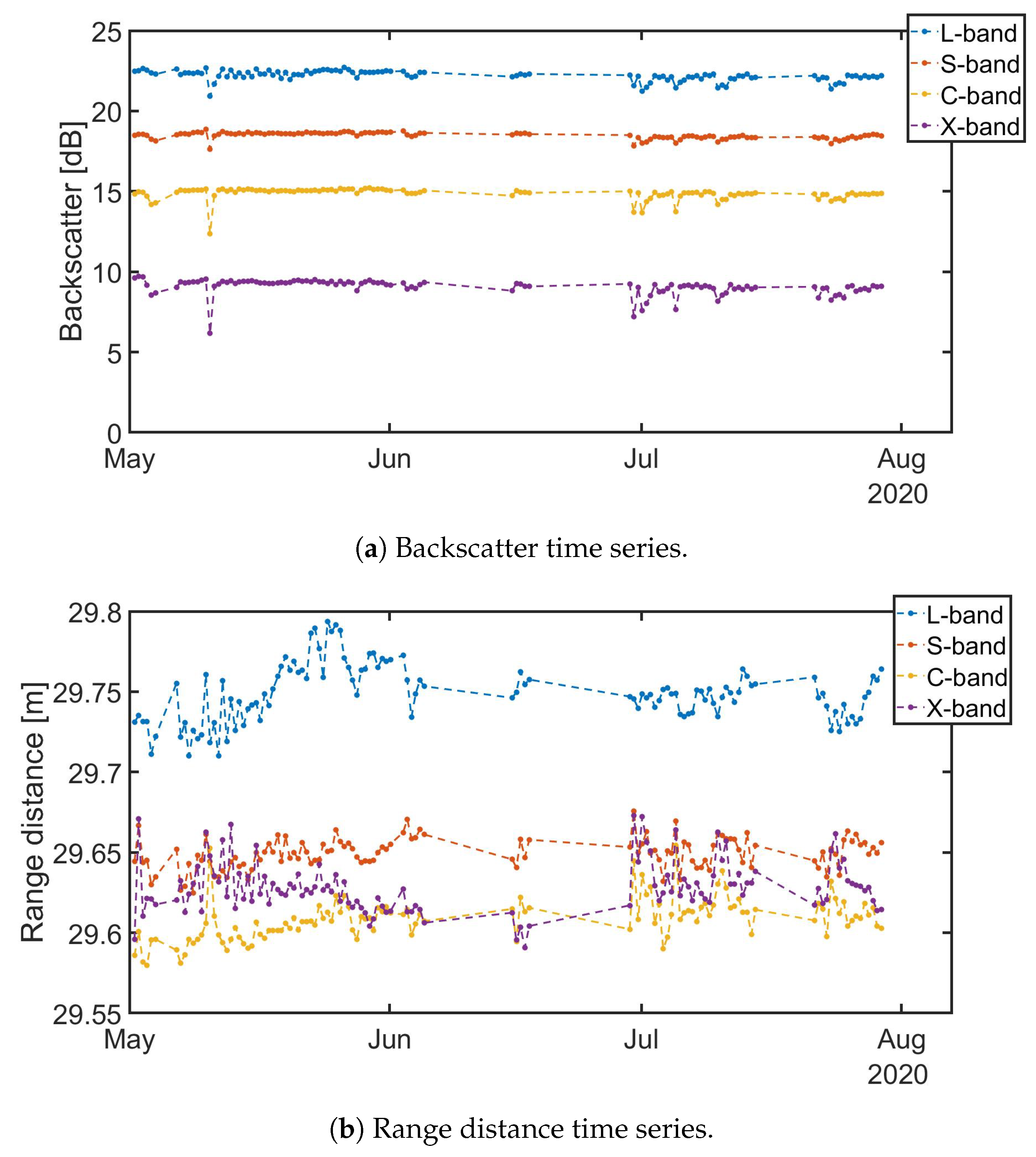
| Band | Average Backscatter (dB) | Standard Deviation (dB) |
|---|---|---|
| L | 22.208 | 0.280 |
| S | 18.497 | 0.161 |
| C | 14.902 | 0.249 |
| X | 9.123 | 0.351 |
| Band | Average Range Distance (m) | Standard Deviation (m) |
|---|---|---|
| L | 29.750 | 0.018 |
| S | 29.649 | 0.009 |
| C | 29.609 | 0.013 |
| X | 29.628 | 0.016 |
Publisher’s Note: MDPI stays neutral with regard to jurisdictional claims in published maps and institutional affiliations. |
© 2020 by the authors. Licensee MDPI, Basel, Switzerland. This article is an open access article distributed under the terms and conditions of the Creative Commons Attribution (CC BY) license (http://creativecommons.org/licenses/by/4.0/).
Share and Cite
Jorge Ruiz, J.; Vehmas, R.; Lemmetyinen, J.; Uusitalo, J.; Lahtinen, J.; Lehtinen, K.; Kontu, A.; Rautiainen, K.; Tarvainen, R.; Pulliainen, J.; et al. SodSAR: A Tower-Based 1–10 GHz SAR System for Snow, Soil and Vegetation Studies. Sensors 2020, 20, 6702. https://0-doi-org.brum.beds.ac.uk/10.3390/s20226702
Jorge Ruiz J, Vehmas R, Lemmetyinen J, Uusitalo J, Lahtinen J, Lehtinen K, Kontu A, Rautiainen K, Tarvainen R, Pulliainen J, et al. SodSAR: A Tower-Based 1–10 GHz SAR System for Snow, Soil and Vegetation Studies. Sensors. 2020; 20(22):6702. https://0-doi-org.brum.beds.ac.uk/10.3390/s20226702
Chicago/Turabian StyleJorge Ruiz, Jorge, Risto Vehmas, Juha Lemmetyinen, Josu Uusitalo, Janne Lahtinen, Kari Lehtinen, Anna Kontu, Kimmo Rautiainen, Riku Tarvainen, Jouni Pulliainen, and et al. 2020. "SodSAR: A Tower-Based 1–10 GHz SAR System for Snow, Soil and Vegetation Studies" Sensors 20, no. 22: 6702. https://0-doi-org.brum.beds.ac.uk/10.3390/s20226702