Absolute Positioning and Orientation of MLSS in a Subway Tunnel Based on Sparse Point-Assisted DR

 , ,
, ,
Abstract
:1. Introduction
2. The Principles of the Method
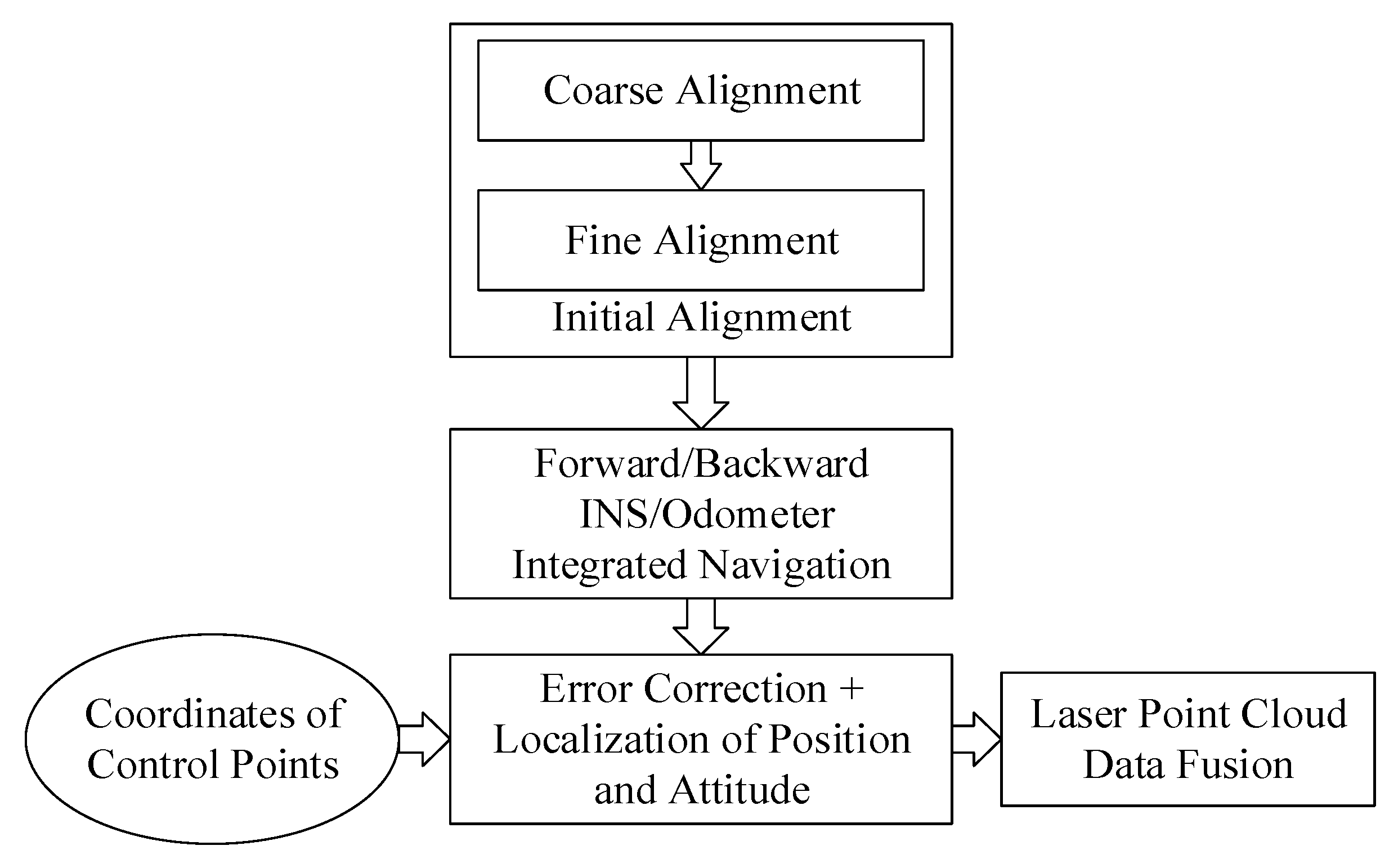
2.1. The Whole Procedure of the Method
2.2. The Initial Alignment Method
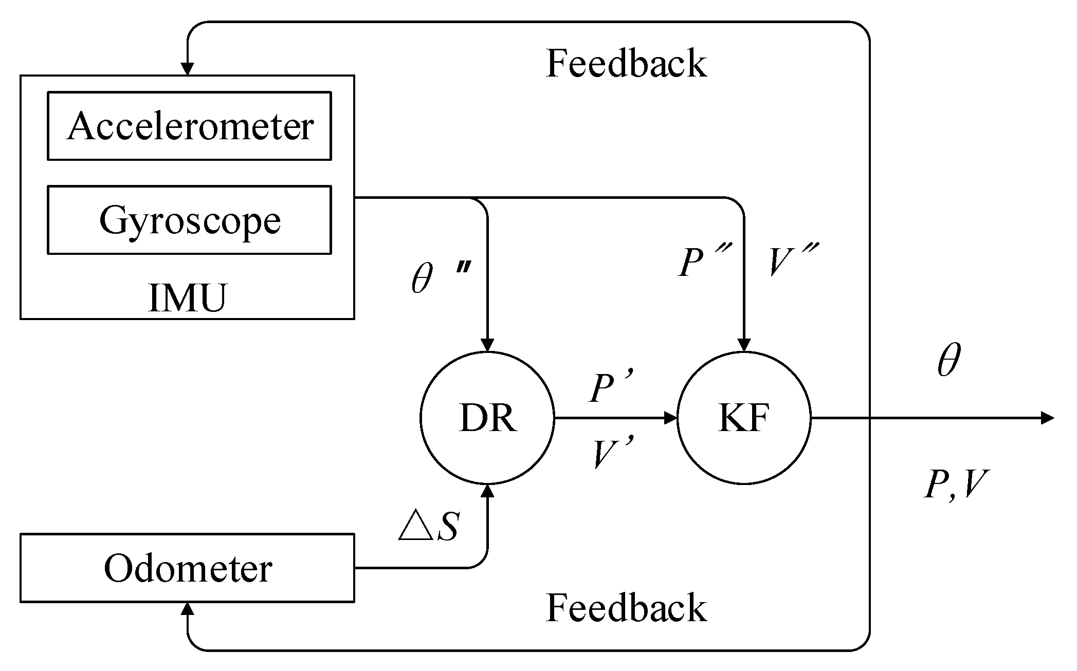
2.3. The INS/Odometer Integrated Navigation Algorithm
2.4. Forward and Backward Dead Reckoning
2.4.1. Unification of the Odometer’s Outputs
2.4.2. Forward DR
2.4.3. Backward DR
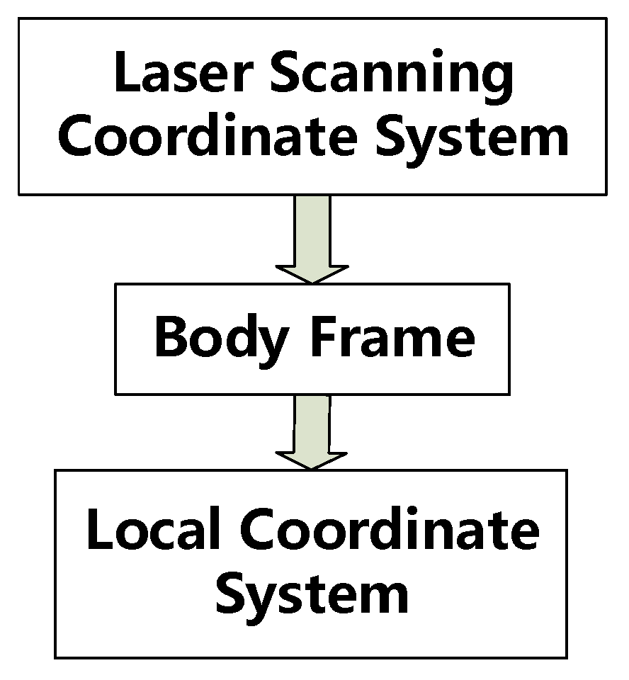
2.5. Conversion Method for Obtaining Absolute Coordinates
2.5.1. Traditional Coordinate Transformation Method
2.5.2. Improved Coordinate Transformation Method
2.5.3. Transformation from NCS to LCS
3. Experiments and Discussions
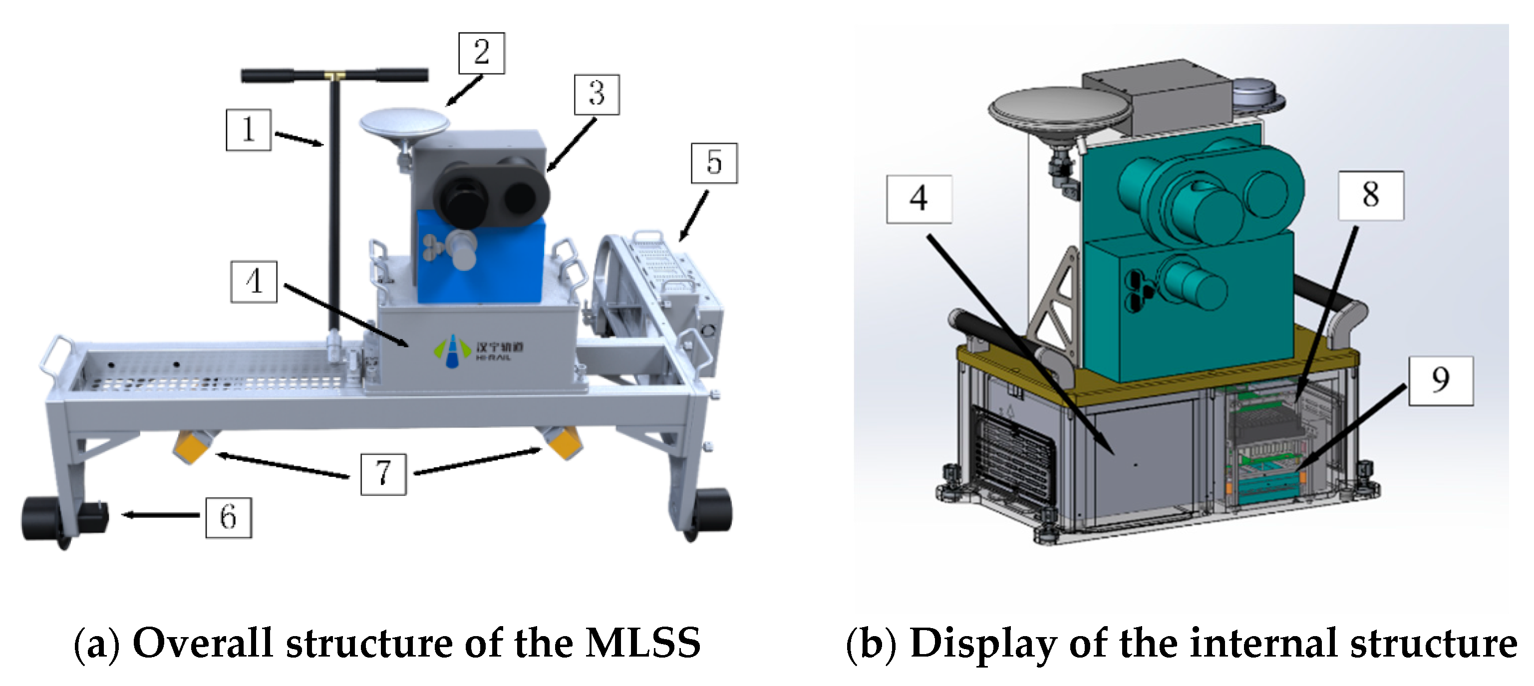
3.1. Information about MLSS
3.2. Experiment in a Tunnel of the Beijing–Zhangjiakou High-Speed Railway
3.2.1. Experimental Conditions
3.2.2. Experimental Results
3.3. Experiments in the Inspection of Subway Tunnels
3.3.1. Experimental Conditions
3.3.2. Experimental Results and Discussions
- (1)
- The data for a 5–6 km long tunnel can be collected in 1 h.
- (2)
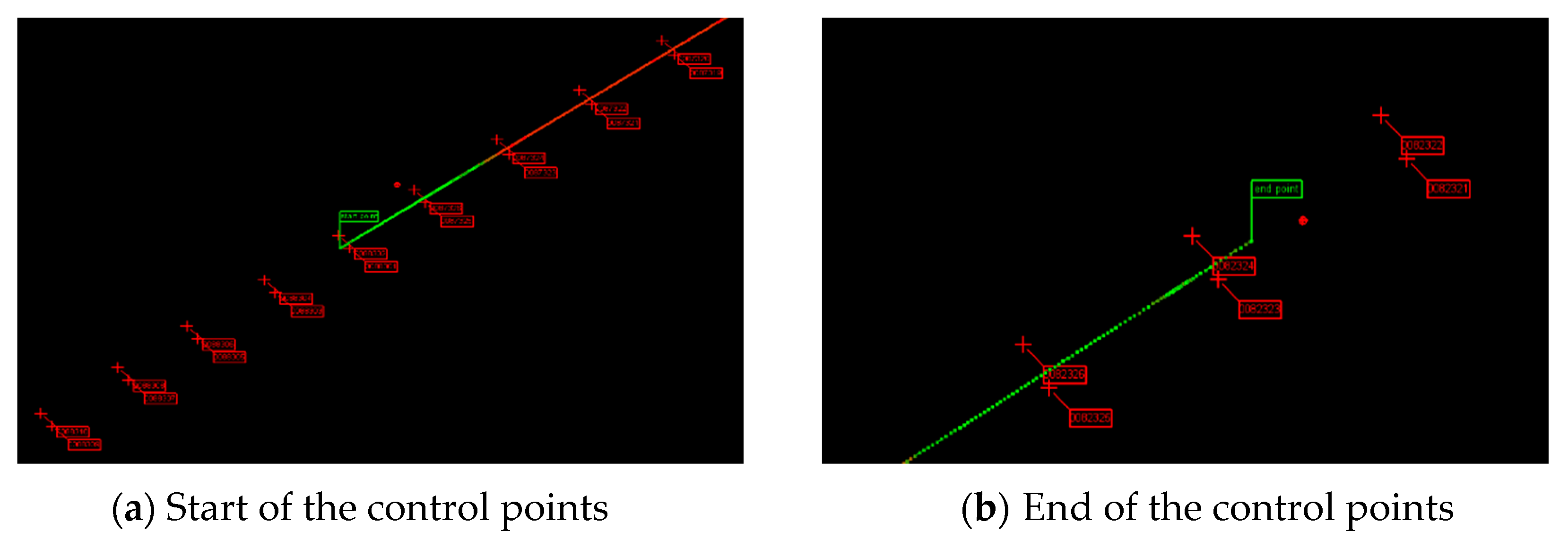
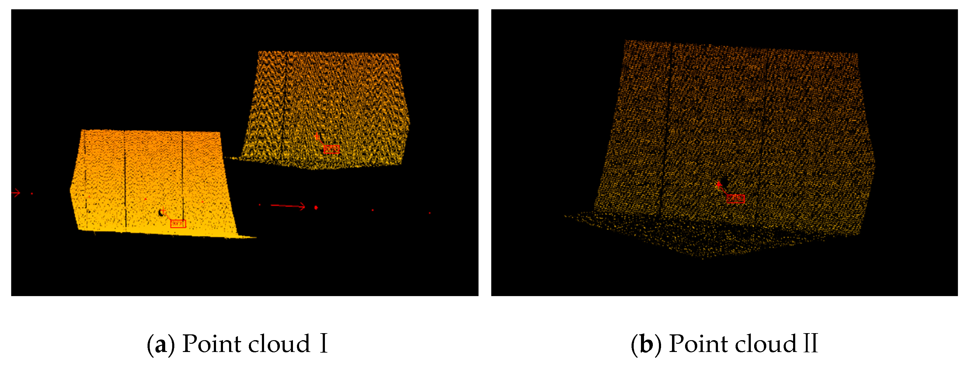
- It takes about 5–10 minutes to fuse the point clouds of the areas around control points, and it only takes a few seconds to select a control point in the point cloud. In this way, we do not need to transform all the point clouds from a body frame to geodetic coordinate system/NCS, which has been described in 2.5.1; this greatly reduces the time required.
- (3)
- After that, the positions and attitudes of the MLSS will be corrected instantly with the algorithm given in Section 2.5.3.
- (4)
- Then, the coordinates of point clouds in the LCS can be directly obtained by using the positions and attitudes, which have been corrected; this step will take about 1 h.
- (5)
- Finally, the inspection of the diseases of a 5–6 km long tunnel based on point clouds will take about 1 h.
4. Conclusions
Author Contributions
Funding
Acknowledgments
Conflicts of Interest
References
- Li, R.; Wu, J.; Zeng, M. Metro Clearance detection based on laser measurement. Urban Rapid Rail Trans. 2007, 5, 70–73. [Google Scholar]
- Gao, X.; Yu, L.; Yang, Z. Subway lining segment faulting detection based on Kinect sensor. In Proceedings of the 2015 IEEE International Conference on Mechatronics and Automation (ICMA), Beijing, China, 2–5 August 2015; pp. 1076–1081. [Google Scholar]
- Mei, W.; Wei, C.; Yu, A. Method and Application of Cross Section Survey of Subway Tunnel by Laser Scanning Car. J. Geomat. 2017, 42. [Google Scholar] [CrossRef]
- Schwarz, K.P.; El-Sheimy, N. Mobile mapping systems–state of the art and future trends. ISPRS Arch. 2004, 35, 10. [Google Scholar]
- Vock, D.M.M.; Jungmichel, M. A Low Budget Mobile Laser Scanning Solution Using on Board Sensors and Field Bus Systems of TODAY’S Consumer Automobiles. ISPRS. Arch. 2011, 34. [Google Scholar] [CrossRef] [Green Version]
- Kim, G.H.; Sohn, H.G.; Song, Y.S. Road Infrastructure Data Acquisition Using a Vehicle-Based Mobile Mapping System. Comput-Aided. Civ. Inf. 2006, 21, 346–356. [Google Scholar] [CrossRef]
- Teo, T.; Chiu, C. Pole-Like Road Object Detection From Mobile Lidar System Using a Coarse-to-Fine Approach. J. Sel. Top. Appl. Earth Obs. Remote Sens. 2015, 8, 4805–4818. [Google Scholar] [CrossRef]
- Yang, M.; Wan, Y.; Liu, X.; Xu, J.; Wei, Z.; Chen, M.; Sheng, P. Laser data based automatic recognition and maintenance of road markings from MLS system. Opt. Laser Technol. 2018, 107, 192–203. [Google Scholar] [CrossRef]
- Tan, K.; Cheng, X.; Ju, Q.; Wu, S. Correction of Mobile TLS Intensity Data for Water Leakage Spots Detection in Metro Tunnels. IEEE Geosci. Remote Sens. Lett. 2016, 13, 1711–1715. [Google Scholar] [CrossRef]
- Shen, B.; Zhang, W.Y.; Qi, D.P.; Wu, X.Y. Wireless Multimedia Sensor Network Based Subway Tunnel Crack Detection Method. Int. J. Distrib. Sens. N. 2015, 11, 184639. [Google Scholar] [CrossRef]
- Ge, R.; Zhu, Y.; Xiao, Y.; Chen, Z. The Subway Pantograph Detection Using Modified Faster R-CNN. In Proceedings of the International Forum of Digital TV and Wireless Multimedia Communication, Shanghai, China, 9–10 November 2016; pp. 197–204. [Google Scholar]
- Li, S.C.; Liu, Z.Y.; Liu, B.; Xu, X.J.; Wang, C.W.; Nie, L.C.; Sun, H.; Song, J.; Wang, S.R. Boulder detection method for metro shield zones based on cross-hole resistivity tomography and its physical model tests. Chin. J. Geotech. Eng. 2015, 37, 446–457. [Google Scholar]
- Zhang, L. Accuracy Improvement of Positioning and Orientation Systems Applied to Mobile Mapping in Complex Environments. Ph.D. Thesis, Wuhan University, Wuhan, China, 2015. [Google Scholar]
- Wu, F. Researches on the Theories and Algorithms of the Error Analysis and Compensation for Integrated Navigation System. Ph.D. Thesis, PLA Information Engineering University, Zhengzhou, China, 2007. [Google Scholar]
- Jing, H.; Slatcher, N.; Meng, X.; Hunter, G. Monitoring capabilities of a mobile mapping system based on navigation qualities. ISPRS Arch. 2016, 625–631. [Google Scholar]
- Barbour, N.; Schmidt, G. Inertial sensor technology trends. IEEE Sens. J. 2001, 1, 332–339. [Google Scholar] [CrossRef]
- Schmidt, G.T. INS/GPS Technology Trends//Advances in navigation sensors and integration technology. NATO RTO Lect. Ser. 2004, 232. [Google Scholar]
- Schmidt, G.; Schmidt, G. GPS/INS technology trends for military systems. In Proceedings of the Guidance, Navigation, and Control Conference, New Orleans, LA, USA, 11–13 August 1997; pp. 1018–1034. [Google Scholar]
- Groves, P.D. Principles of GNSS, Inertial, and Multi-sensor Integrated Navigation Systems. Trans. Aerosp. Electron. Syst. 2015, 30, 26–27. [Google Scholar] [CrossRef]
- Liu, J.; Cai, B.; Wang, J. Map-aided BDS/INS Integration Based Track Occupancy Estimation Method for Railway Trains. J. China Railway Soc. 2014, 36, 49–58. [Google Scholar]
- Larsen, M.B. High performance Doppler-inertial navigation-experimental results. In Proceedings of the OCEANS 2000 MTS/IEEE Conference and Exhibition, Providence, RI, USA, 11–14 September 2000; pp. 1449–1456. [Google Scholar]
- Luck, T.; Meinke, P.; Eisfeller, B.; Kreye, C.; Stephanides, J. Measurement of Line Characteristics and Track Irregularities by Means of DGPS and INS. In Proceedings of the International Symposium on Kinematic Systems in Geodesy, Geomatics and Navigation, Banff, AB, Canada, 5–8 June 2001. [Google Scholar]
- Chiang, K.W.; Chang, H.W. Intelligent Sensor Positioning and Orientation through Constructive Neural Network-Embedded INS/GPS Integration Algorithms. Sensors 2010, 10, 9252–9285. [Google Scholar] [CrossRef] [Green Version]
- Luck, T.; Lohnert, E.; Eissfeller, B.; Meinke, P. Track irregularity measurement using an INS-GPS integration technique. WIT Trans. Built Environ. 2000, 105–114. [Google Scholar] [CrossRef]
- Chen, Q.; Niu, X.; Zhang, Q.; Cheng, Y. Railway track irregularity measuring by GNSS/INS integration. Navig. J. Inst. Navig. 2015, 62, 83–93. [Google Scholar] [CrossRef]
- Chen, Q.; Niu, X.; Zuo, L.; Zhang, T.; Xiao, F.; Liu, Y.; Liu, J. A railway track geometry measuring trolley system based on aided INS. Sensors 2018, 18, 538. [Google Scholar] [CrossRef] [Green Version]
- Gao, Z.; Ge, M.; Li, Y.; Shen, W.; Zhang, H.; Schuh, H. Railway irregularity measuring using Rauch–Tung–Striebel smoothed multi-sensors fusion system: quad-GNSS PPP, IMU, odometer, and track gauge. GPS Solut. 2018, 22, 36. [Google Scholar] [CrossRef]
- Han, J.; Lo, C. Adaptive time-variant adjustment for the positioning errors of a mobile mapping platform in GNSS-hostile areas. Surv. Rev. 2017, 49, 9–14. [Google Scholar] [CrossRef]
- Shi, Z. Advanced Mobile Mapping System Development with Integration of Laser Data, Stereo Images and other Sensor Data. Citeseer 2014. [Google Scholar]
- Strasdat, H.; Montiel, J.M.; Davison, A.J. Visual SLAM: Why filter? Image Vis. Comput. 2012, 30, 65–77. [Google Scholar] [CrossRef]
- Li, Q.; Chen, Z.; Hu, Q.; Zhang, L. Laser-aided INS and odometer navigation system for subway track irregularity measurement. J. Surv. Eng. Asce 2017, 143, 04017014. [Google Scholar] [CrossRef]
- Mao, Q.; Zhang, L.; Li, Q.; Hu, Q.; Yu, J.; Feng, S.; Ochieng, W.; Gong, H. A least squares collocation method for accuracy improvement of mobile LiDAR systems. Remote Sens. 2015, 7, 7402–7424. [Google Scholar] [CrossRef] [Green Version]
- Jiang, Q.; Wu, W.; Li, Y.; Jiang, M. Millimeter scale track irregularity surveying based on ZUPT-aided INS with sub-decimeter scale landmarks. Sensors 2017, 17, 2083. [Google Scholar] [CrossRef] [Green Version]
- Sun, P.; Li, G.; Zhang, Z.; Wang, X. Research on SINS Static Alignment Algorithm and Experiment. In Proceedings of the 2015 International Conference on Network and Information Systems for Computers (ICNISC), Wuhan, China, 23–25 January 2015; pp. 305–308. [Google Scholar]
- Roberto, V.; Ivan, D.; Jizhong, X. Keeping a good attitude: A quaternion-based orientation filter for imus and MARGs. Sensors 2015, 15, 19302–19330. [Google Scholar]
- Wang, X.; Shen, G. A fast and accurate initial alignment method for strapdown inertial navigation system on stationary base. J. Control Theory Appl. 2005, 3, 145–149. [Google Scholar] [CrossRef]
- Wu, Y.; Zhang, H.; Wu, M.; Hu, X.; Hu, D. Observability of Strapdown INS Alignment: A Global Perspective. IEEE Trans. Aerosp. Electron. Syst. 2012, 48, 78–102. [Google Scholar]
- Kaygısız, B.H.; Şen, B. In-motion alignment of a low-cost GPS/INS under large heading error. J. Navig. 2015, 68, 355–366. [Google Scholar] [CrossRef] [Green Version]
- Chang, L.; Qin, F.; Jiang, S. Strapdown Inertial Navigation System Initial Alignment Based on Modified Process Model. IEEE Sens. J. 2019, 19, 6381–6391. [Google Scholar] [CrossRef]
- Shin, E.H. Accuracy Improvement of Low Cost INS/GPS for Land Applications. Master’s Thesis, The University of Calgary, Calgary, AB, Canada, December 2001. [Google Scholar]
- Bar-Itzhack, I.Y.; Berman, N. Control theoretic approach to inertial navigation systems. J. Guid. Control. Dynam. 1987, 10, 1442–1453. [Google Scholar]
- Li, Z.; Wang, J.; Li, B.; Gao, J.; Tan, X. GPS/INS/Odometer integrated system using fuzzy neural network for land vehicle navigation applications. J. Navig. 2014, 67, 967–983. [Google Scholar] [CrossRef] [Green Version]
- Wang, W.; Wang, D. Land vehicle navigation using odometry/INS/vision integrated system. In Proceedings of the 2008 IEEE Conference on Cybernetics and Intelligent Systems, Chengdu, China, 21–24 September 2008; pp. 754–759. [Google Scholar]
- Trimble, M. Dead reckoning. Cns Spectrums 2002, 7, 565. [Google Scholar] [CrossRef] [PubMed]
- Yan, G. Research on Strapdown Inertial Navigation Algorithm and Vehicle Integrated Navigation System. Master’s Thesis, Northwestern Polytechnic University, Xi’an, China, 2004. [Google Scholar]
- Yan, G. Research on Vehicle Autonomous Positioning and Orientation System. Ph.D. Thesis, Northwestern Polytechnic University, Xi’an, China, 2006. [Google Scholar]
- Fu, Q. Key Technologies for Vehicular Positioning and Orientation System. Ph.D. Thesis, Northwestern Polytechnic University, Xi’an, China, 2015. [Google Scholar]
- Jimenez, A.R.; Seco, F.; Prieto, C.; Guevara, J. A comparison of Pedestrian Dead-Reckoning algorithms using a low-cost MEMS IMU. In Proceedings of the 2009 IEEE International Symposium on Intelligent Signal Processing, Budapest, Hungary, 26–28 August 2009; pp. 37–42. [Google Scholar]
- Dong, C.; Mao, Q.; Ren, X.; Kou, D.; Qin, J.; Hu, W. Algorithms and instrument for rapid detection of rail surface defects and vertical short-wave irregularities based on fog and odometer. IEEE Access 2019, 7, 31558–31572. [Google Scholar] [CrossRef]
- Gongmin, Y.; Weisheng, Y.; Demin, X. On Reverse Navigation Algorithm and its Application to SINS Gyro-compass In-movement Alignment. In Proceedings of the 27th Chinese Control Conference, Kunming, China, 16–18 July 2008; pp. 724–729. [Google Scholar]
- Yoon, H.; Ham, Y.; Golparvar-Fard, M.; Spencer, B.F., Jr. Forward-backward approach for 3d event localization using commodity smartphones for ubiquitous context-aware applications in civil and infrastructure engineering. Comput. Aided Civ. Inf. 2016, 31, 245–260. [Google Scholar] [CrossRef]
- Li, W.; Wang, J.; Li, G.; Zhang, Y. Robust estimation and precision analysis on four-parameter coordinate transformation. J. Hebei U. Univ. 2016, 38, 24–28. [Google Scholar]
- Wu, Y.; Liu, J.; Ge, H.Y. Comparison of Total Least Squares and Least Squares for Four-and Seven-parameter Model Coordinate Transformation. J. Appl. Geodesy 2016, 10, 259–266. [Google Scholar] [CrossRef]


| Emission Frequency | Scanning Frequency | Scanning Range | Measuring Distance | Distance Error (Reflectivity = 90%) | Efficiency |
|---|---|---|---|---|---|
| p/s | 200 r/s | 360° | 0.5–119 m | 2 mm (distance = 80 m) | 3–5 km/h |
| Gyro Bias | Gyro Bias Stability | Gyro Bias Repeatability | Gyro Random Walk | Accelerometer Bias | Accelerometer Bias Repeatability |
|---|---|---|---|---|---|
| ≤±0.1°/h | ≤0.01°/h | ≤0.01°/h | ≤0.003°/h1/2 | ≤0.00005 g | ≤0.00005 g |
| Horizontal | Elevation | 3-D | |
|---|---|---|---|
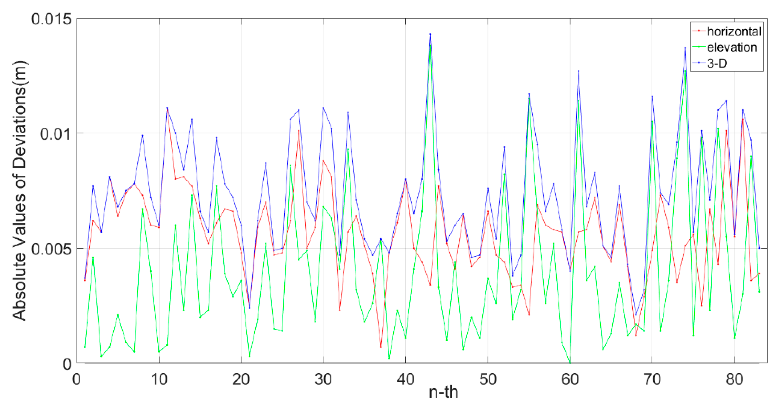
| Maximum (m) | 0.011 | 0.013 | 0.014 |
| Minimum (m) | 0.0007 | 0.000 | 0.002 |
| RMS (m) | 0.006 | 0.005 | 0.008 |
| Horizontal Error (m) | Elevation Error (m) | 3-D RMS (m) | ||||
|---|---|---|---|---|---|---|
| Maximum | Average | RMS | Maximum | Average | RMS | |
| 0.016 | 0.008 | 0.005 | 0.043 | 0.026 | 0.022 | 0.023 |
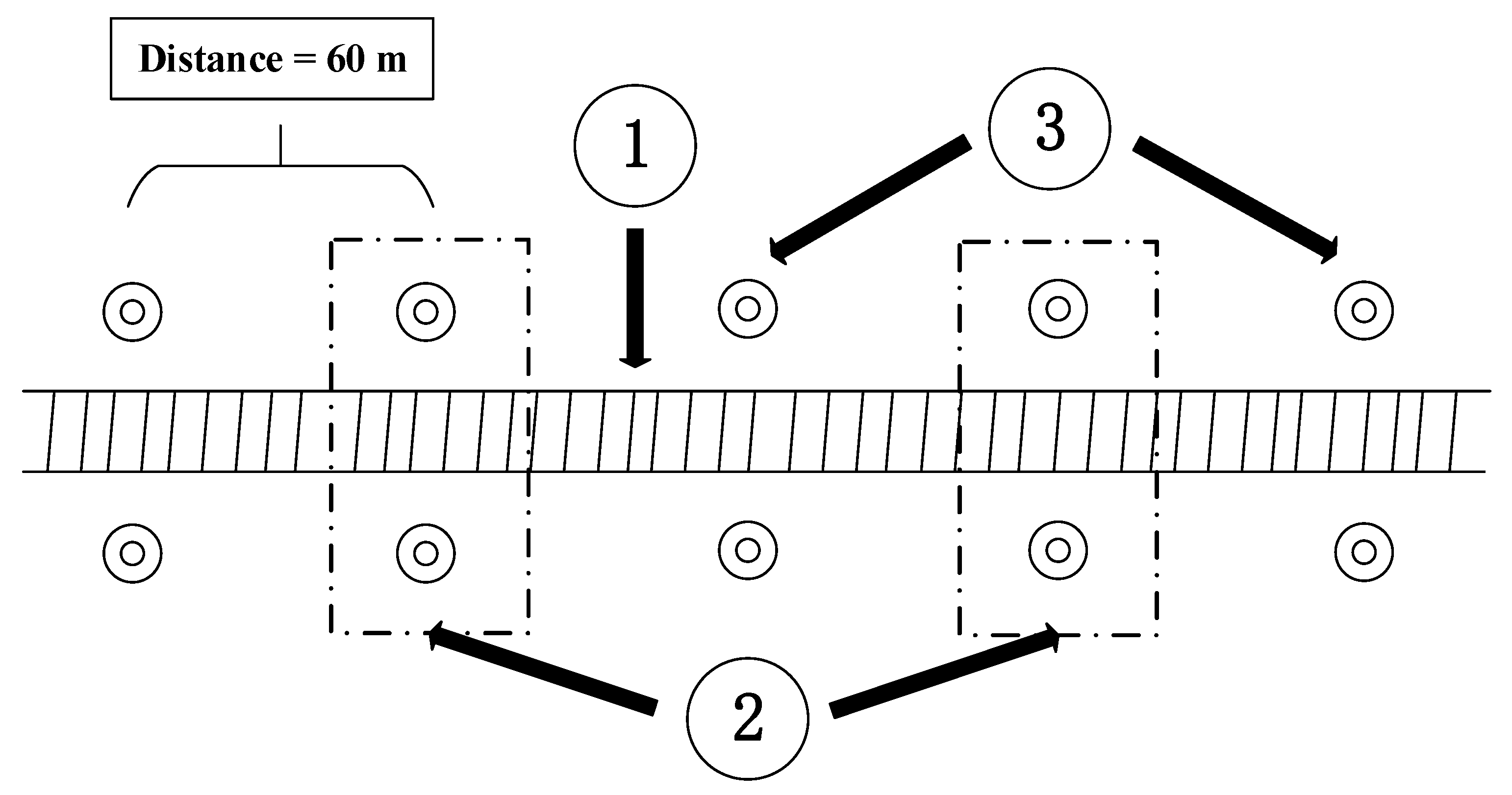
| Distance Interval (m) | Horizontal Error (m) | Elevation Error (m) | 3-D RMS (m) | ||||
|---|---|---|---|---|---|---|---|
| Maximum | Average | RMS | Maximum | Average | RMS | ||
| 60 | 0.010 | 0.005 | 0.004 | 0.013 | 0.007 | 0.002 | 0.004 |
| 120 | 0.010 | 0.004 | 0.004 | 0.018 | 0.009 | 0.004 | 0.006 |
| 240 | 0.010 | 0.004 | 0.004 | 0.012 | 0.002 | 0.006 | 0.007 |
| 480 | 0.010 | 0.004 | 0.004 | 0.012 | 0.002 | 0.007 | 0.008 |
© 2020 by the authors. Licensee MDPI, Basel, Switzerland. This article is an open access article distributed under the terms and conditions of the Creative Commons Attribution (CC BY) license (http://creativecommons.org/licenses/by/4.0/).
Share and Cite
Wang, Q.; Tang, C.; Dong, C.; Mao, Q.; Tang, F.; Chen, J.; Hou, H.; Xiong, Y. Absolute Positioning and Orientation of MLSS in a Subway Tunnel Based on Sparse Point-Assisted DR. Sensors 2020, 20, 645. https://0-doi-org.brum.beds.ac.uk/10.3390/s20030645
Wang Q, Tang C, Dong C, Mao Q, Tang F, Chen J, Hou H, Xiong Y. Absolute Positioning and Orientation of MLSS in a Subway Tunnel Based on Sparse Point-Assisted DR. Sensors. 2020; 20(3):645. https://0-doi-org.brum.beds.ac.uk/10.3390/s20030645
Chicago/Turabian StyleWang, Qian, Chao Tang, Cuijun Dong, Qingzhou Mao, Fei Tang, Jianping Chen, Haiqian Hou, and Yonggang Xiong. 2020. "Absolute Positioning and Orientation of MLSS in a Subway Tunnel Based on Sparse Point-Assisted DR" Sensors 20, no. 3: 645. https://0-doi-org.brum.beds.ac.uk/10.3390/s20030645