Multi-objective Informative Frequency Band Selection Based on Negentropy-induced Grey Wolf Optimizer for Fault Diagnosis of Rolling Element Bearings


Abstract
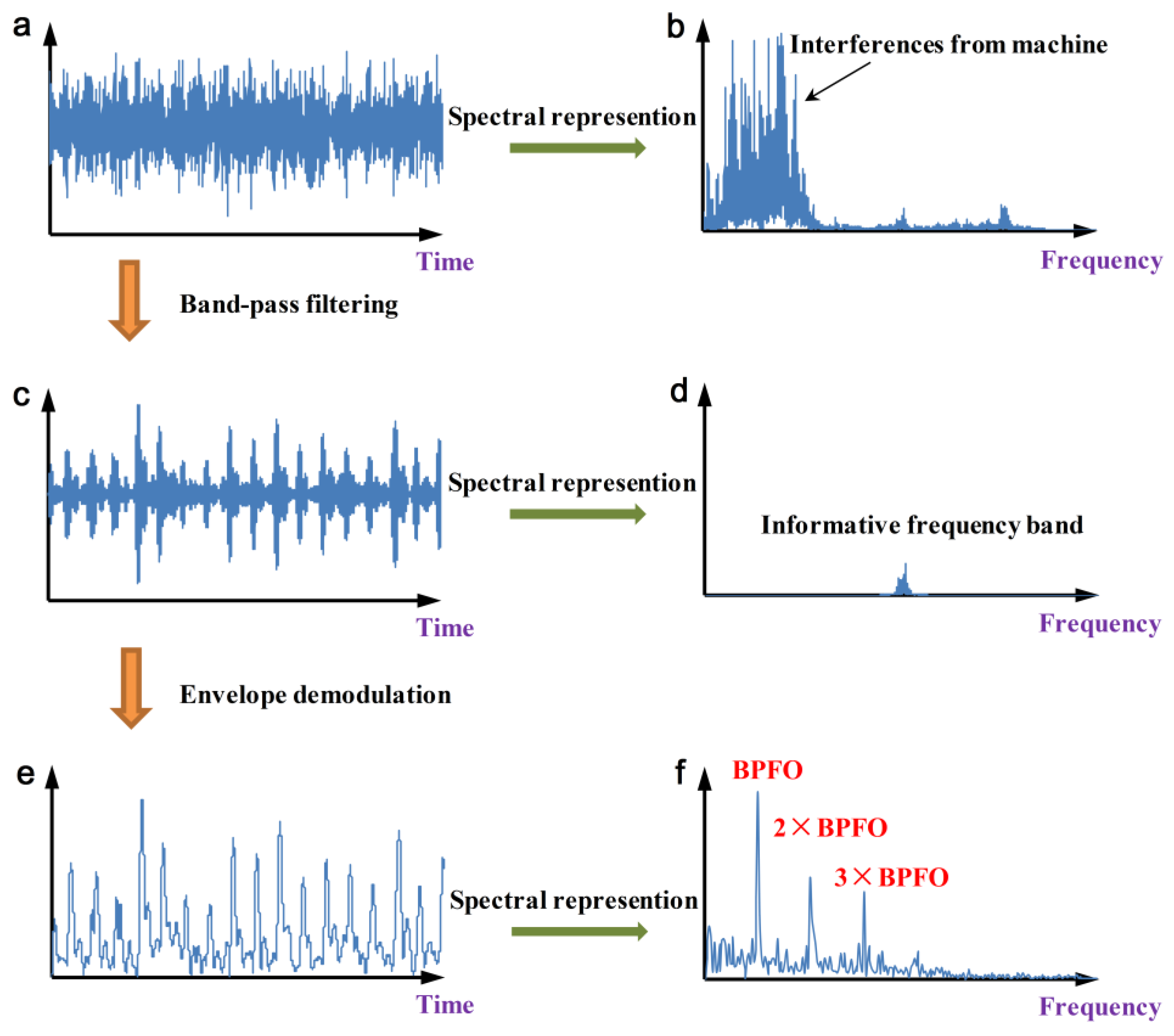
:1. Introduction
2. Methodologies
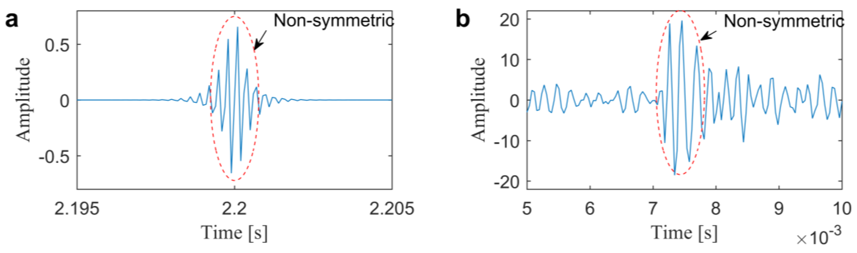
2.1. Wavelet Transform and Anti-symmetric Real Laplace Wavelet Filter
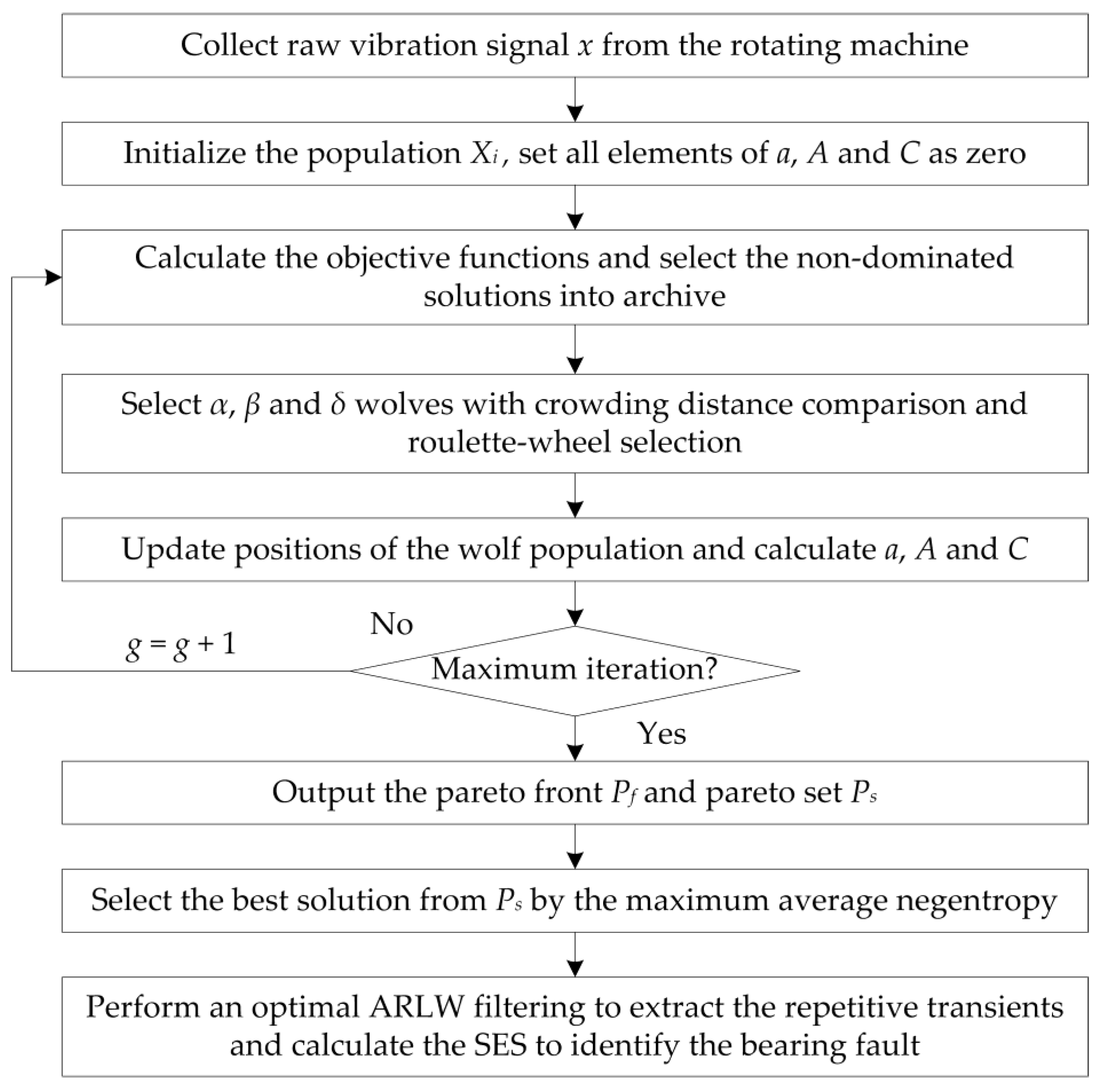
2.2. Multi-objective Optimization and Multi-objective Grey Wolf Optimizer
- Encircling prey:where denotes the current iteration, is the position of prey and is the position of the wolf. and are two coefficients that are defined as:where is linearly decreased from 2 to 0 during the iterations, and are random vectors in .
- Hunting:where , and indicate the best three positions attained by , and wolves, , and represent the distances between the best three wolves and the wolf population. Subsequently, the position of the population will update under the leadership of , and :where , and are all generated from Equation (14) and they corresponded to , and wolves, respectively.
- Attacking prey: When it indicates an exploration behavior of the search agent and otherwise indicates an exploitation one i.e., to attack the prey.In handling multi-objective optimization, another two operations are also introduced. Firstly, an external archive is employed to restore the non-dominated solutions with a competitive update strategy that is similar to that in [38]. Secondly, a leader selection mechanism is formulated with the help of crowding distance comparison [39] and roulette-wheel selection. The detailed introduction can be referred in [35]. The pseudo code of MOGWO algorithm is given, as below Algorithm 1:
Algorithm 1. Multi-objective grey wolf optimizer (MOGWO). Begin Initialize the grey wolf population Initialize and Calculate the objective values of each wolf, put the non-dominated solutions into the archive Select the best three wolves from the archive and save as and g = 1 while (g < maximum number of iterations) for each wolf Update the position by Equations (16)–(22) end for Update and Calculate the objective values of each wolf, update the archive Update and g = g + 1 end while Return archive
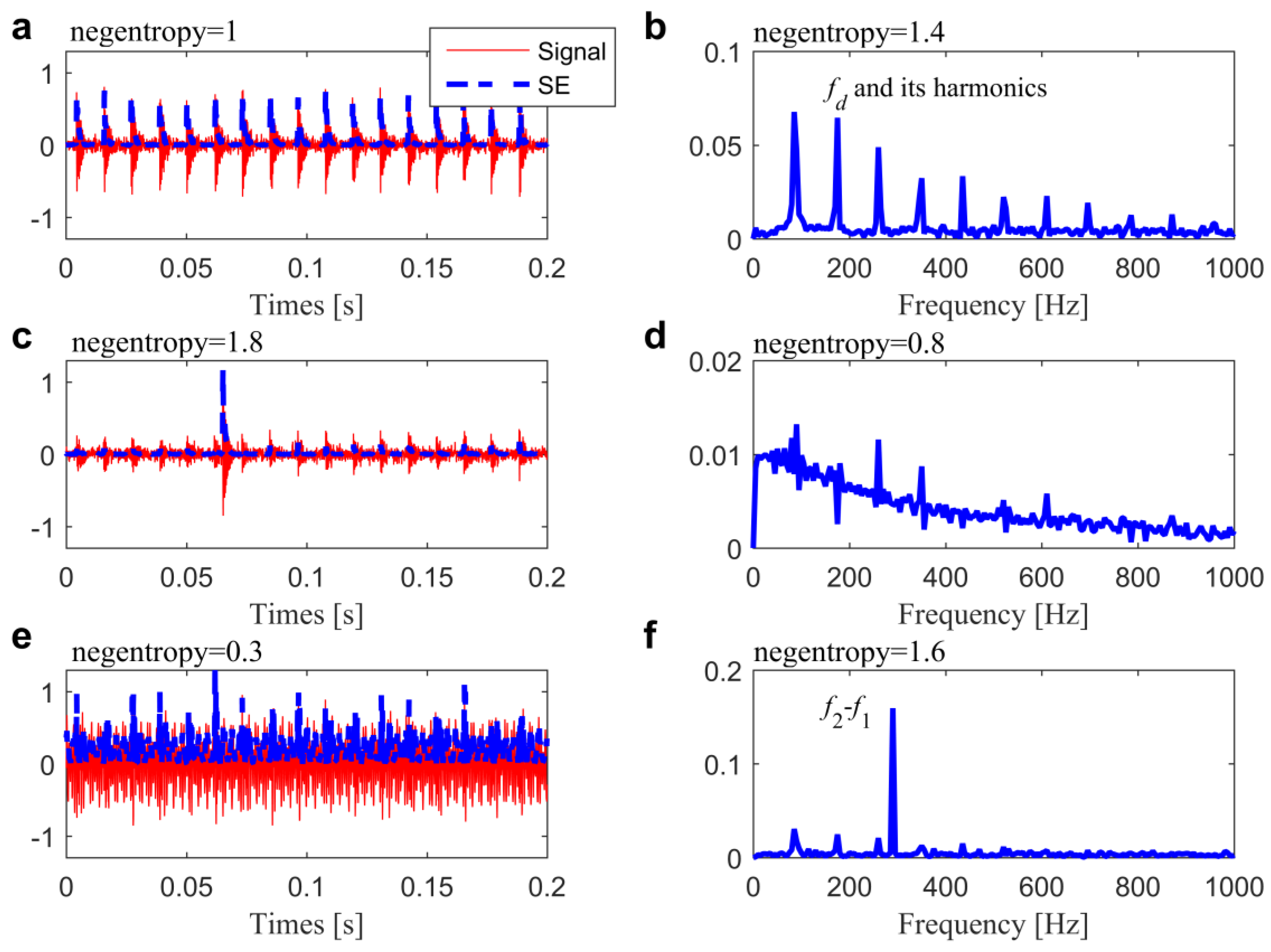
2.3. Proposed Negentropy-Induced IFB Selection Method
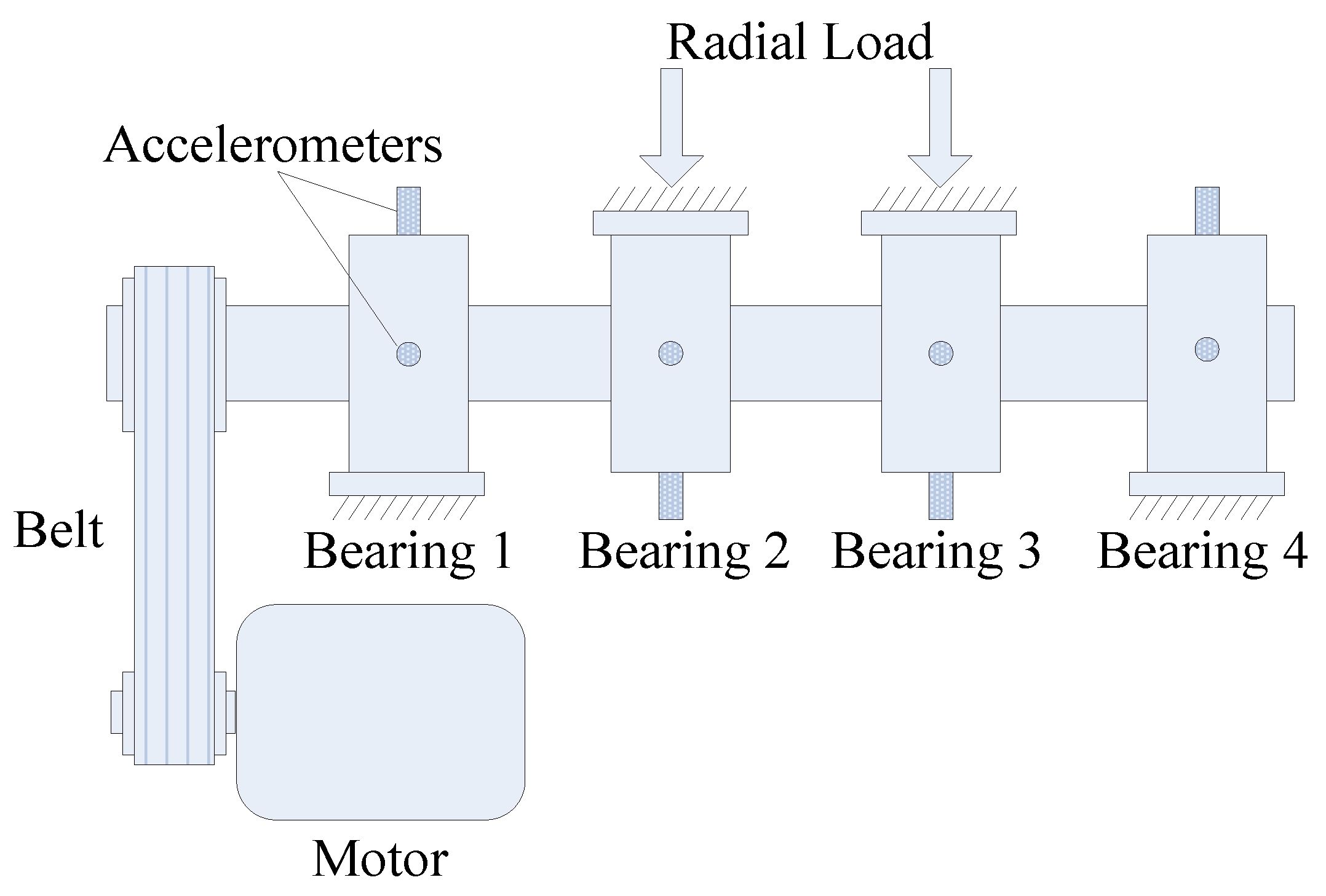
3. Experimental Studies
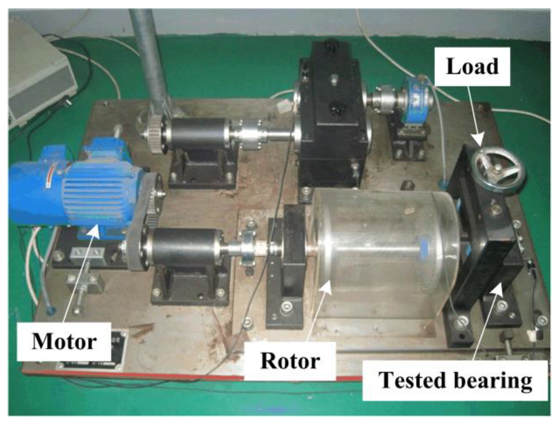
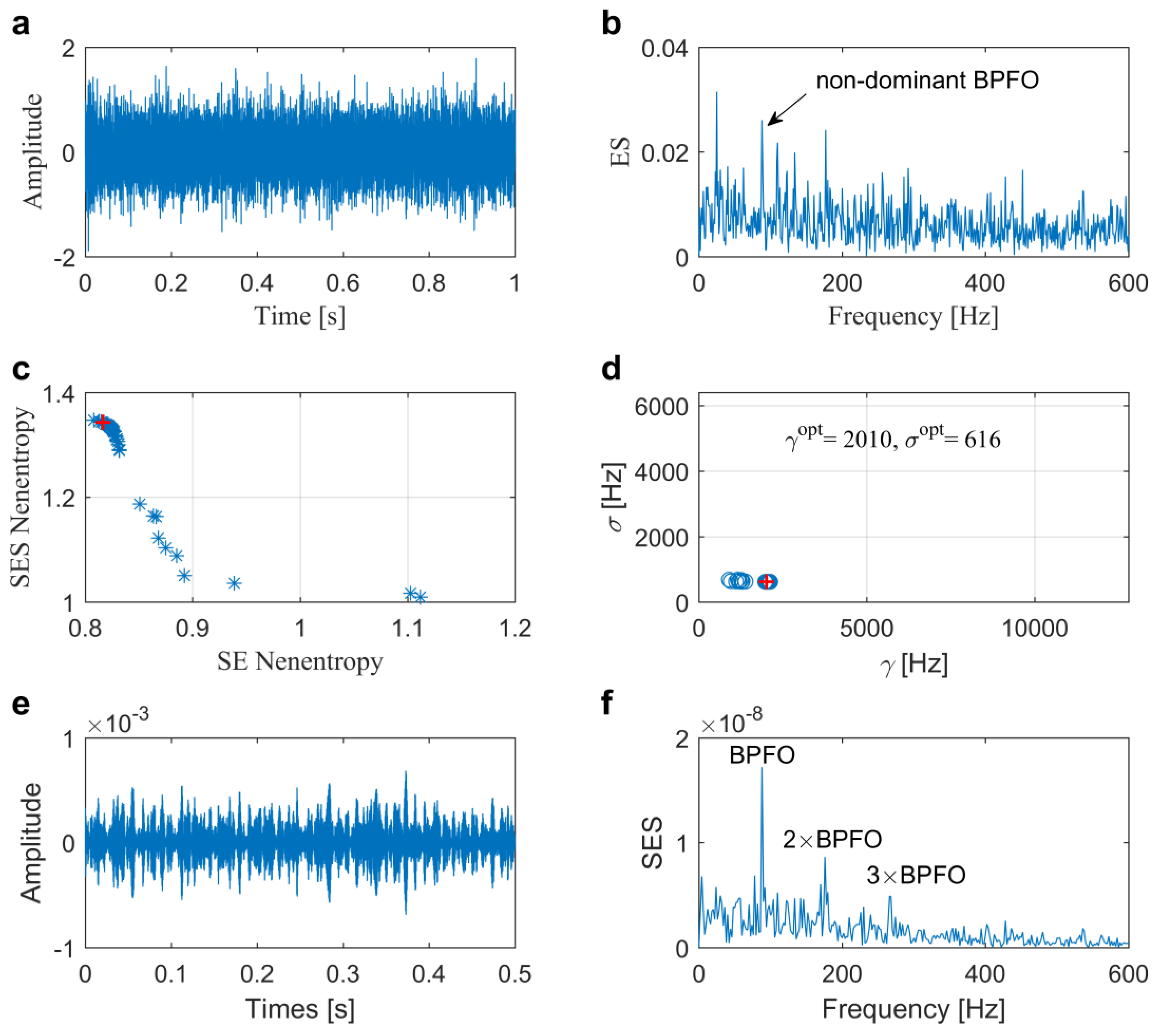
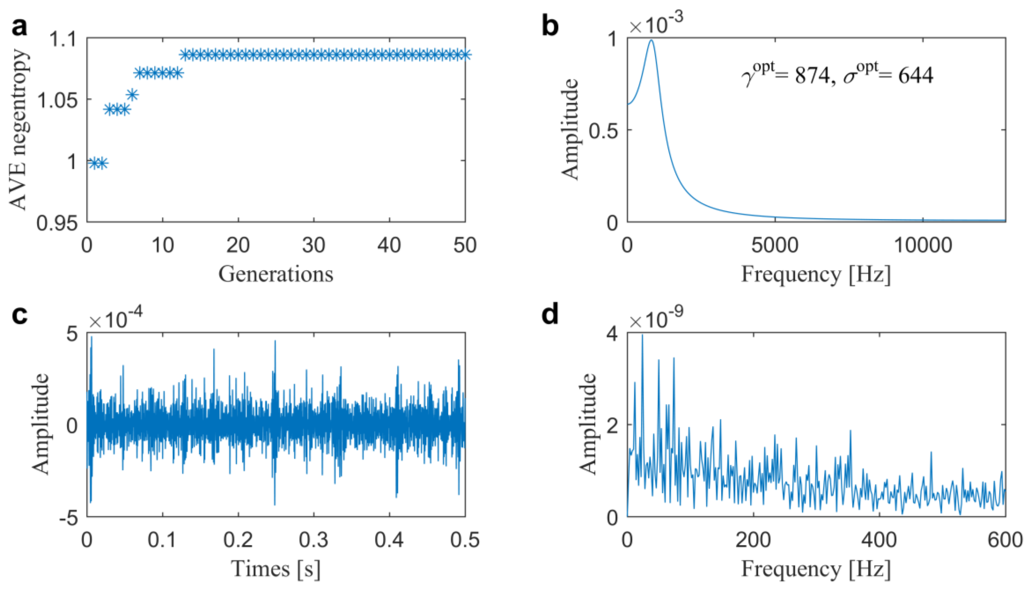
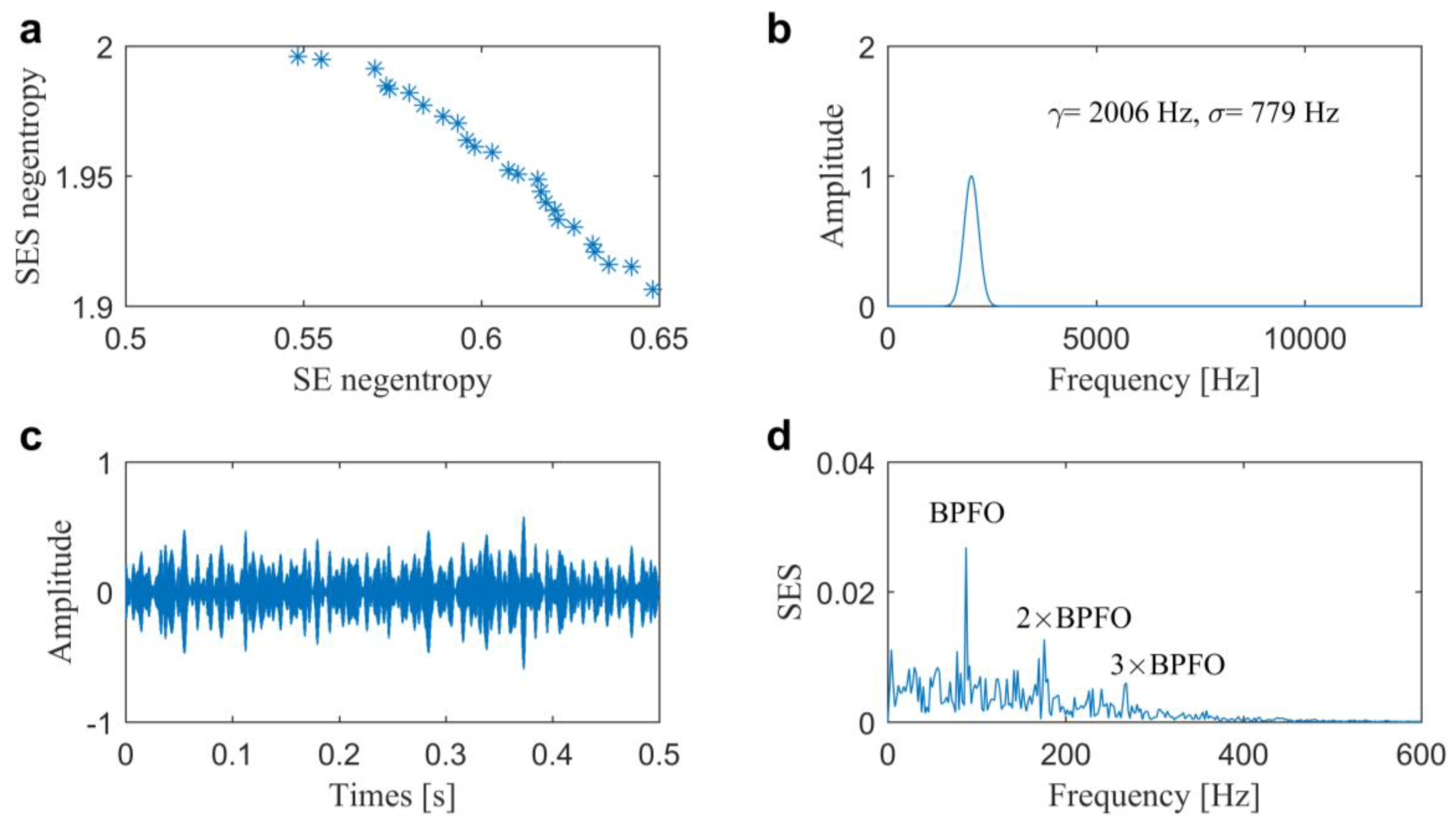
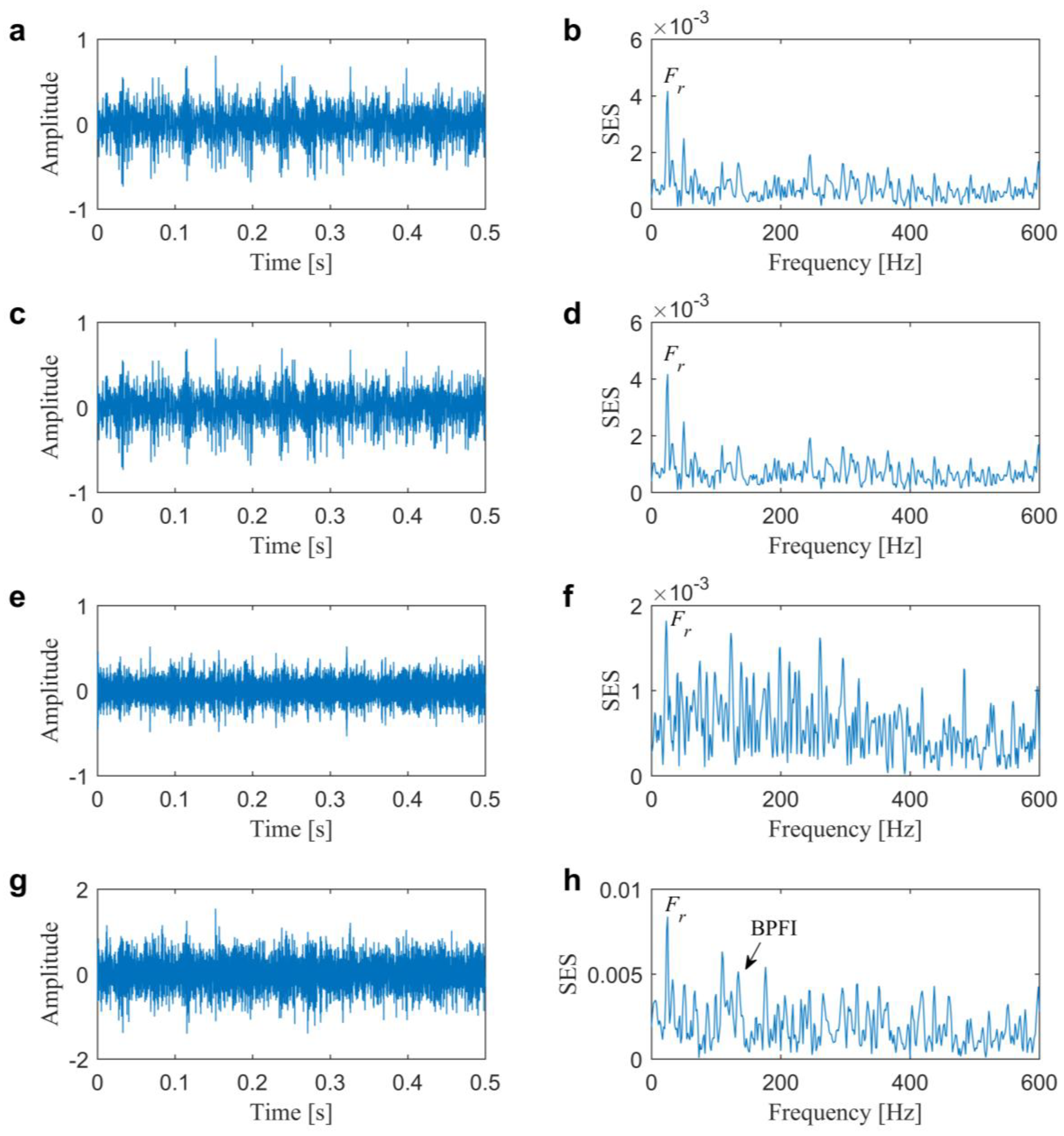
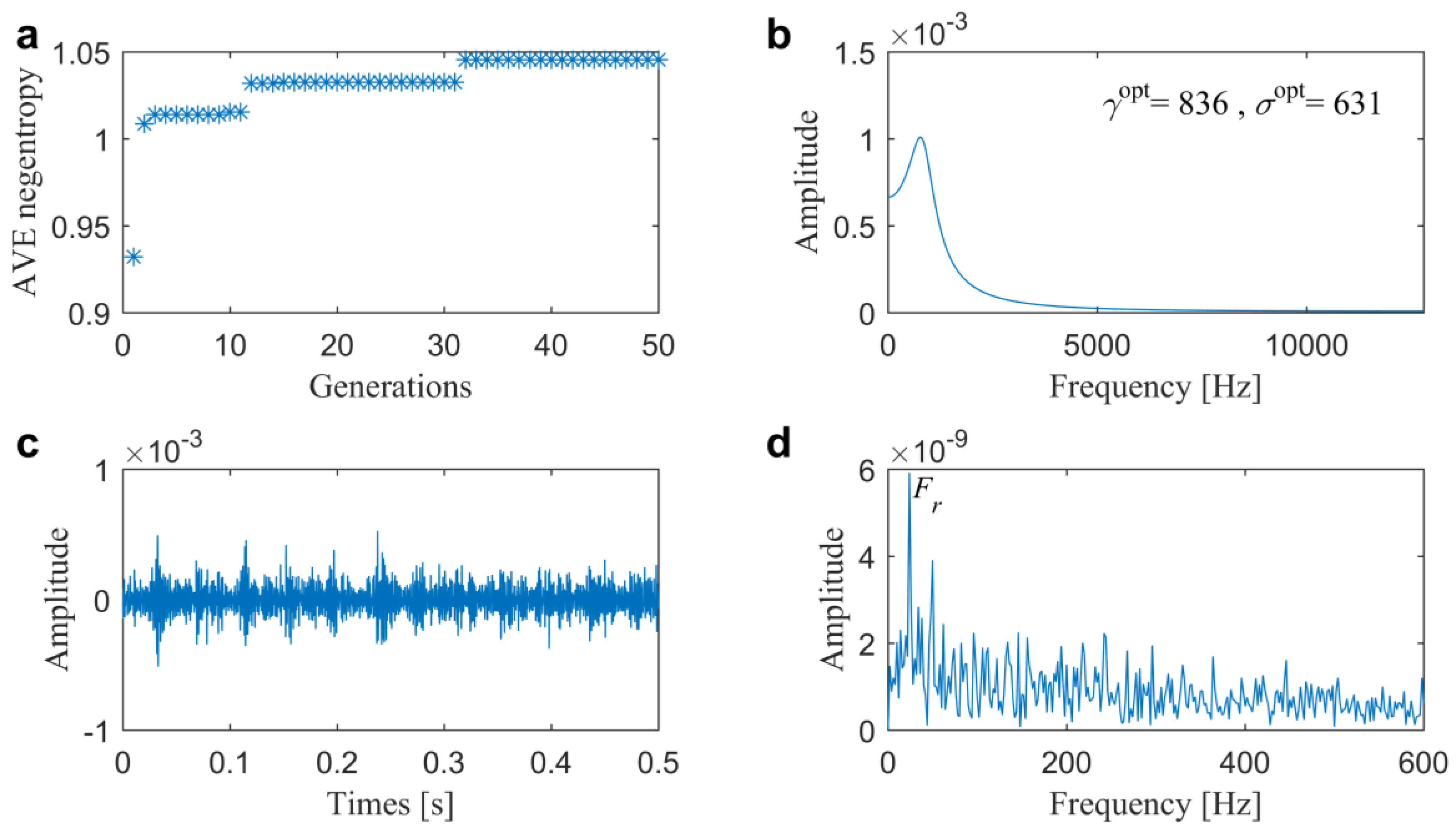
3.1. Case 1: Detection of Slight Artificial Outer Race Fault in a Ball Bearing
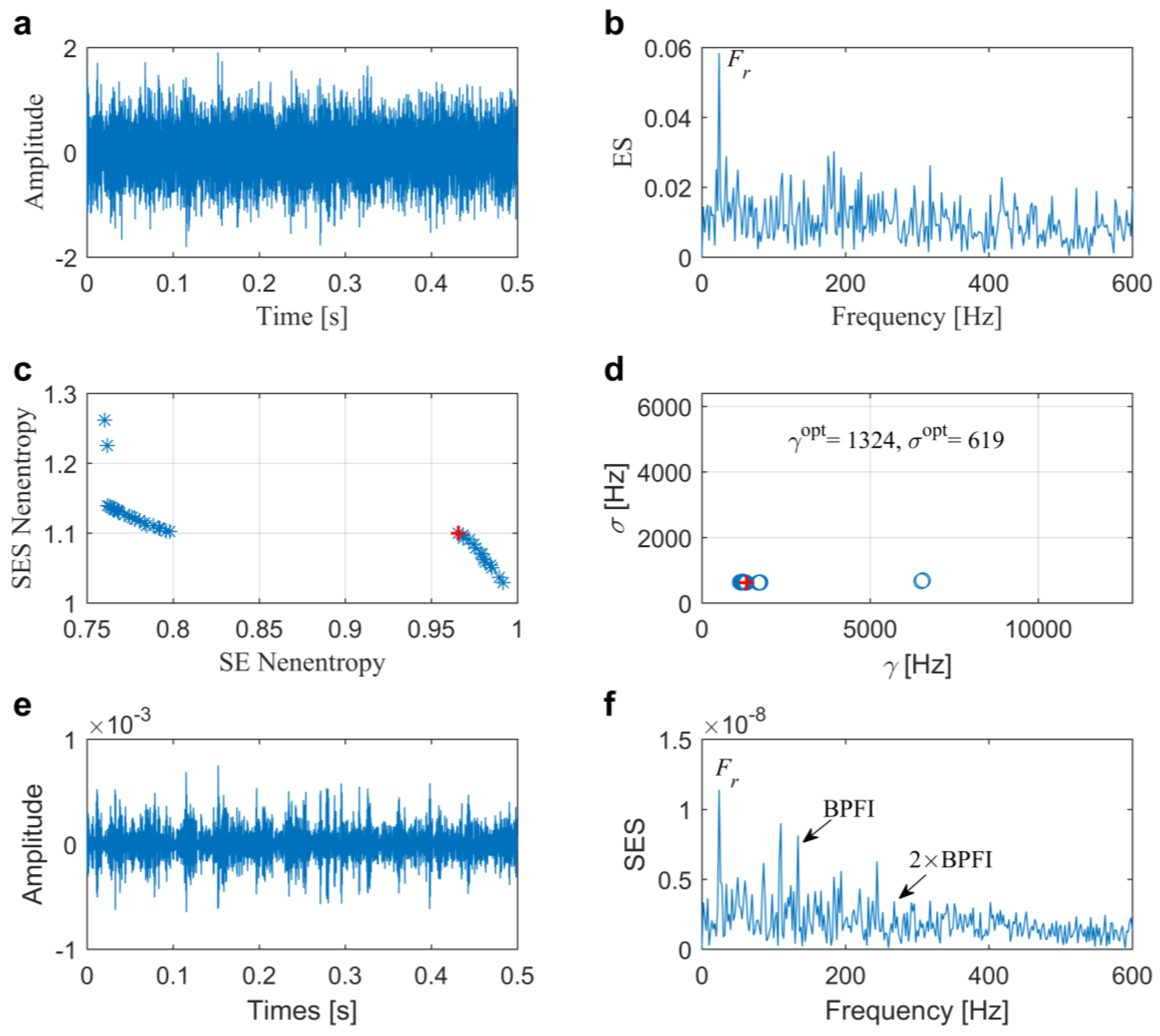
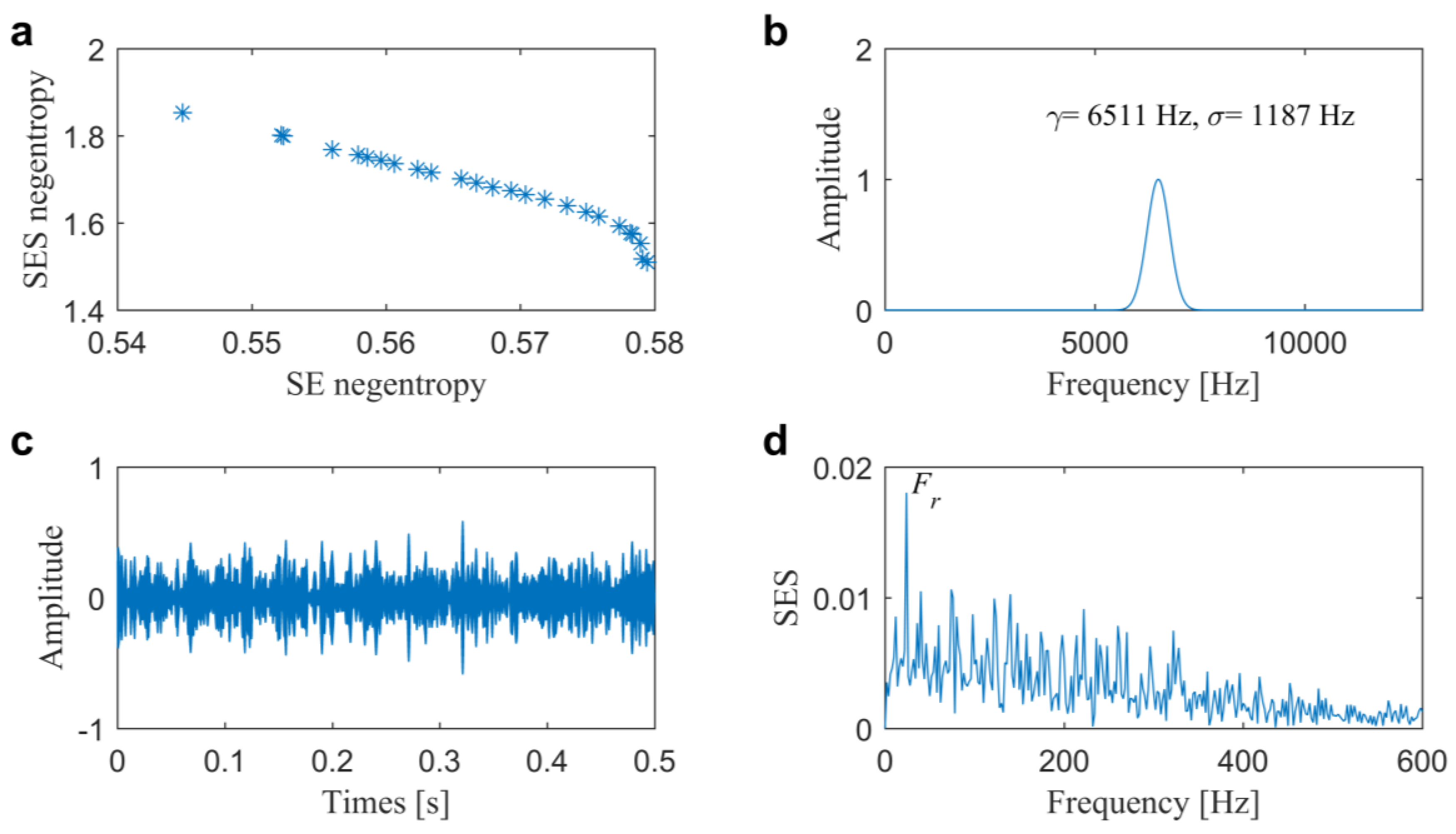
3.2. Case 2: Detection of Slight Artificial Inner Race Fault in a Ball Bearing
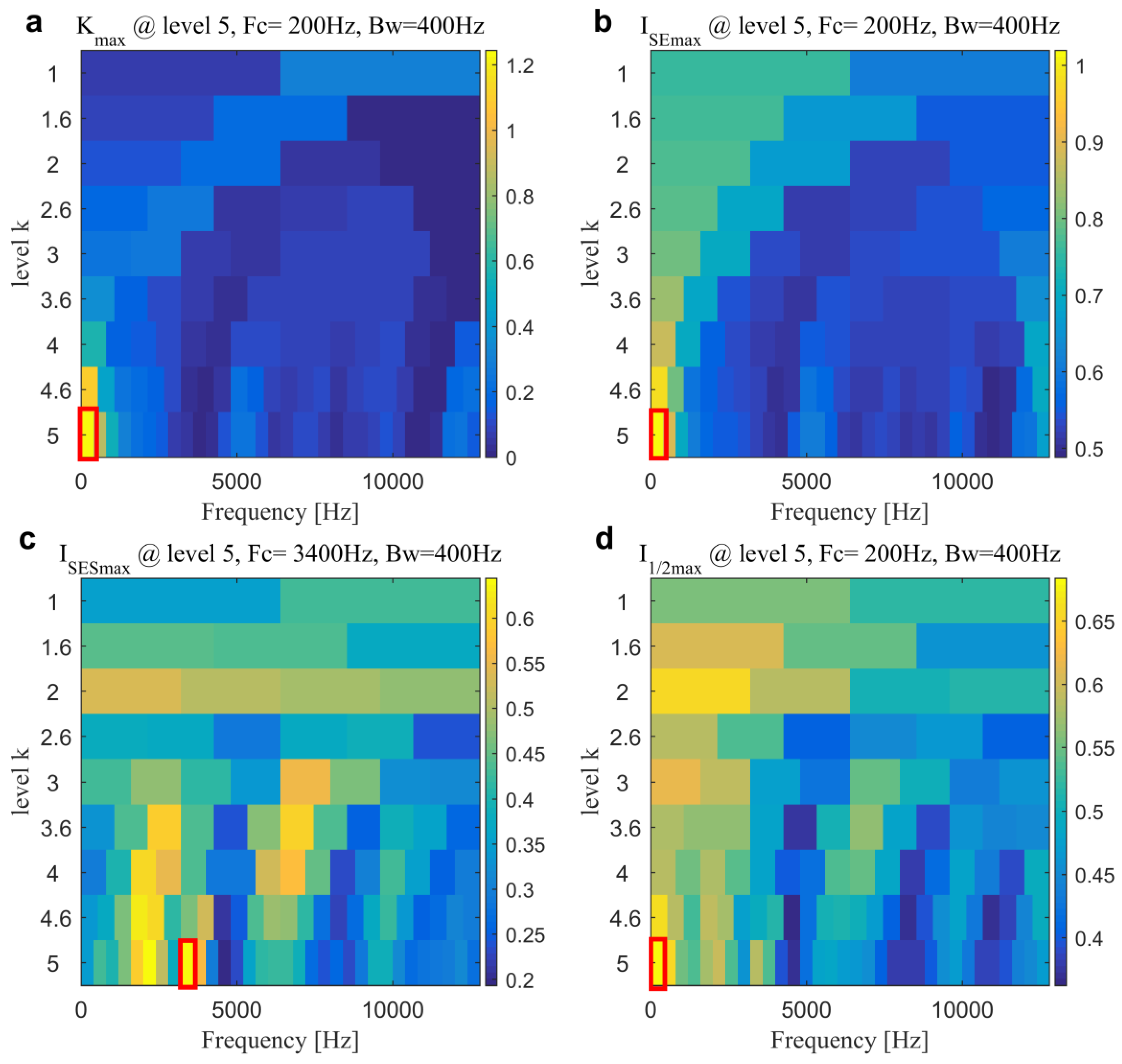
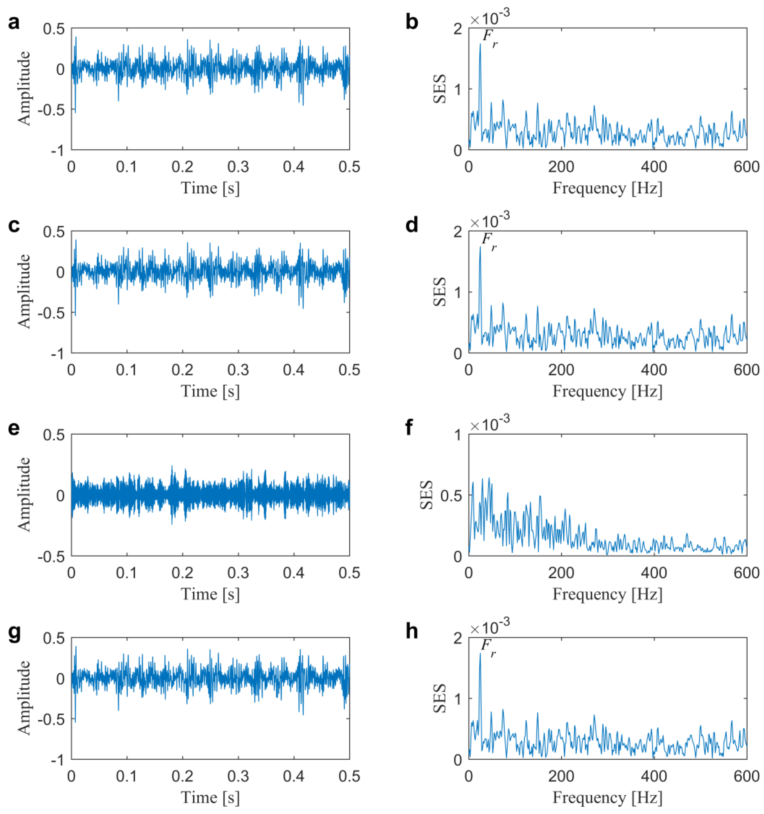
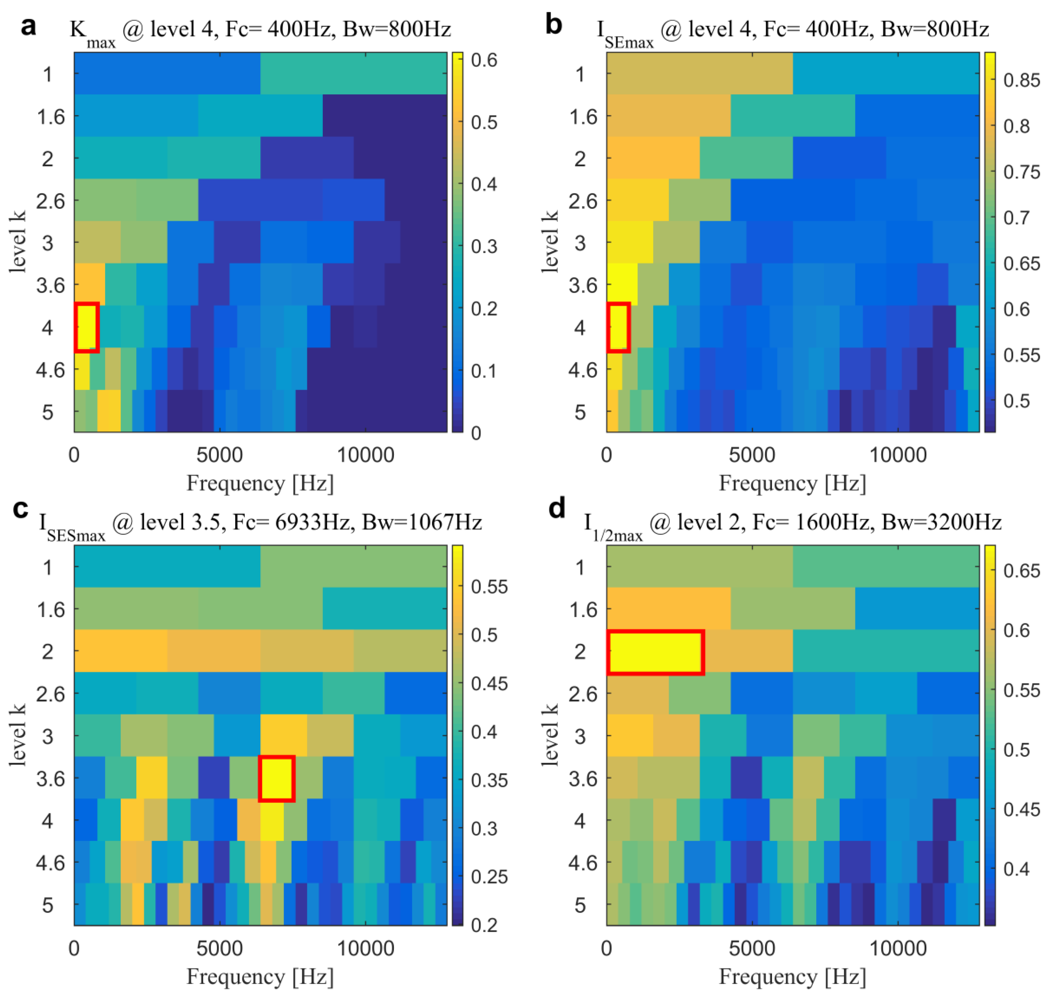
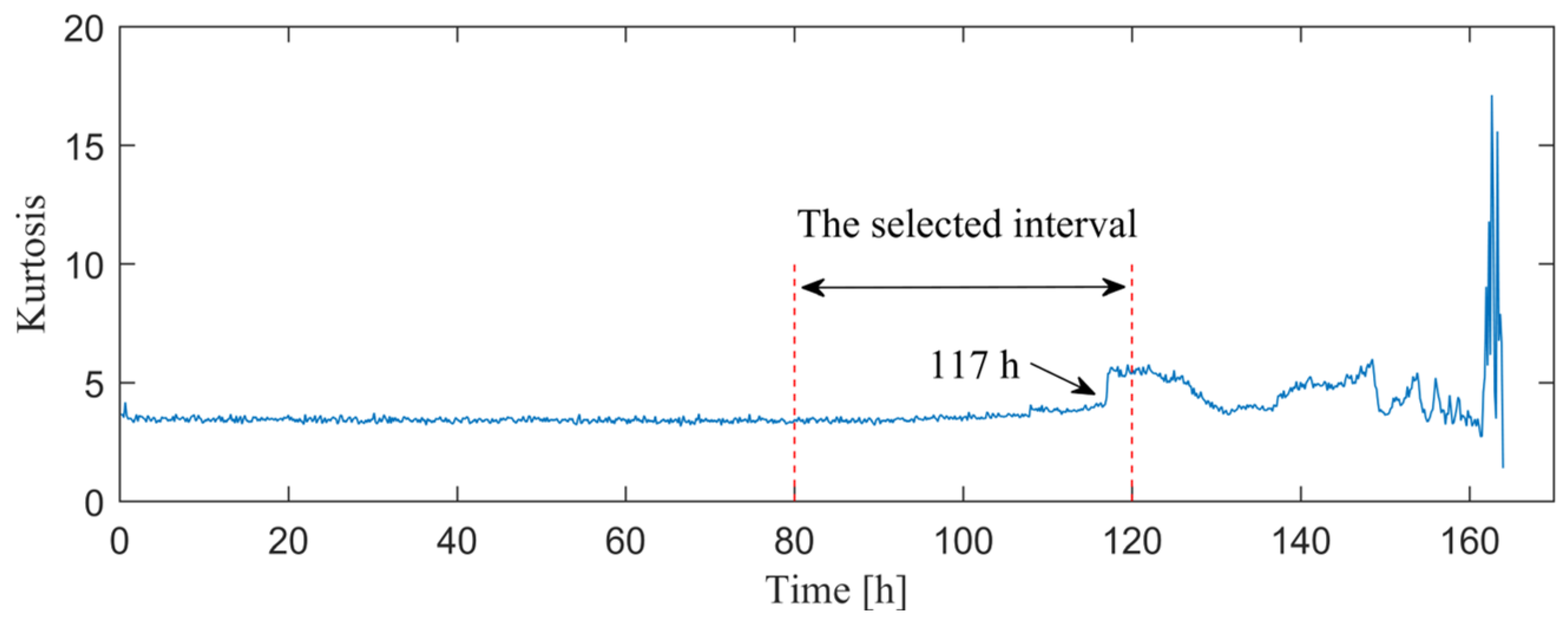
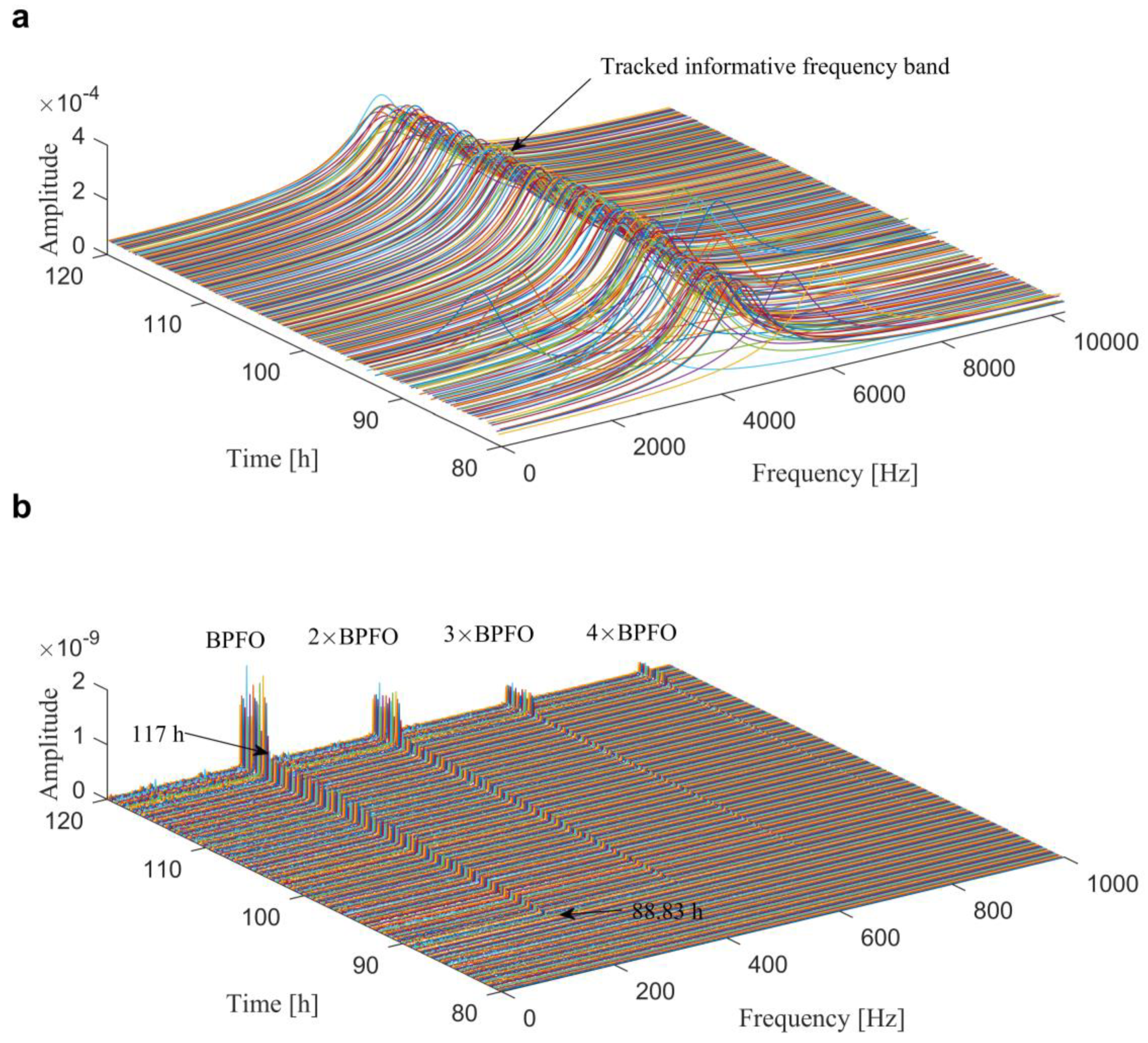
3.3. Case 3: Tracking IFB for a Condition Monitoring Data Set
4. Conclusions
Author Contributions
Funding
Conflicts of Interest
References
- Yi, C.; Wang, D.; Fan, W.; Tsui, K.L.; Lin, J. EEMD-based steady-state indexes and their applications to condition monitoring and fault diagnosis of railway axle bearings. Sensors 2018, 18, 704. [Google Scholar] [CrossRef] [Green Version]
- Wang, Y.; Liu, F.; Zhu, A. Bearing Fault Diagnosis Based on a Hybrid Classifier Ensemble Approach and the Improved Dempster-Shafer Theory. Sensors 2019, 19, 2097. [Google Scholar] [CrossRef] [Green Version]
- Randall, R.B. Vibration-Based Condition Monitoring: Industrial, Aerospace and Automotive Applications, 3rd ed.; John Wiley & Sons: Chichester, UK, 2011. [Google Scholar]
- Kiral, Z.; Karagülle, H. Simulation and analysis of vibration signals generated by rolling element bearing with defects. Tribol. Int. 2003, 36, 667–678. [Google Scholar] [CrossRef]
- McFadden, P.D.; Smith, J.D. Model for the vibration produced by a single point defect in a rolling element bearing. J. Sound Vib. 1984, 96, 69–82. [Google Scholar] [CrossRef]
- Obuchowski, J.; Wyłomańska, A.; Zimroz, R. Selection of informative frequency band in local damage detection in rotating machinery. Mech. Syst. Signal Process. 2014, 48, 138–152. [Google Scholar] [CrossRef]
- Nguyen, H.; Kim, J.; Kim, J.M. Optimal sub-band analysis based on the envelope power Spectrum for effective fault detection in bearing under variable, low speeds. Sensors 2018, 18, 1389. [Google Scholar] [CrossRef] [Green Version]
- Jin, Y.; Liu, Z.; Peng, D.; Kang, J.; Ding, J. Informative frequency band selection based on a new indicator: Accuracy rate. J. Intell. Fuzzy Syst. 2018, 34, 3487–3498. [Google Scholar] [CrossRef]
- Liu, Z.; Jin, Y.; Zuo, M.J.; Peng, D. ACCUGRAM: A novel approach based on classification to frequency band selection for rotating machinery fault diagnosis. ISA Trans. 2019, 95, 346–357. [Google Scholar] [CrossRef]
- Wodecki, J.; Kruczek, P.; Bartkowiak, A.; Zimroz, R.; Wyłomańska, A. Novel method of informative frequency band selection for vibration signal using Nonnegative Matrix Factorization of spectrogram matrix. Mech. Syst. Signal Process. 2019, 130, 585–596. [Google Scholar] [CrossRef]
- Ni, Q.; Wang, K.; Zheng, J. Rolling element bearings fault diagnosis based on a novel optimal frequency band selection scheme. IEEE Access 2019, 7, 80748–80766. [Google Scholar] [CrossRef]
- Antoni, J.; Randall, R.B. The spectral kurtosis: Application to the vibratory surveillance and diagnostics of rotating machines. Mech. Syst. Signal Process. 2006, 20, 308–331. [Google Scholar] [CrossRef]
- Antoni, J. Fast computation of the kurtogram for the detection of transient faults. Mech. Syst. Signal Process. 2007, 21, 108–124. [Google Scholar] [CrossRef]
- Lei, Y.; Lin, J.; He, Z.; Zi, Y. Application of an improved kurtogram method for fault diagnosis of rolling element bearings. Mech. Syst. Signal Process. 2011, 25, 1738–1749. [Google Scholar] [CrossRef]
- Yu, G.; Li, C.; Zhang, J. A new statistical modeling and detection method for rolling element bearing faults based on alpha–stable distribution. Mech. Syst. Signal Process. 2013, 41, 155–175. [Google Scholar] [CrossRef]
- Peter, W.T.; Wang, D. The design of a new sparsogram for fast bearing fault diagnosis: Part 1 of the two related manuscripts that have a joint title as “Two automatic vibration-based fault diagnostic methods using the novel sparsity measurement—Parts 1 and 2”. Mech. Syst. Signal Process. 2013, 40, 499–519. [Google Scholar]
- Miao, Y.; Zhao, M.; Lin, J. Improvement of kurtosis-guided-grams via Gini index for bearing fault feature identification. Meas. Sci. Technol. 2017, 28, 125001. [Google Scholar] [CrossRef]
- Wang, D. Spectral L2/L1 norm: A new perspective for spectral kurtosis for characterizing non-stationary signals. Mech. Syst. Signal Process. 2018, 104, 290–293. [Google Scholar] [CrossRef]
- Wang, D. Some further thoughts about spectral kurtosis, spectral L2/L1 norm, spectral smoothness index and spectral Gini index for characterizing repetitive transients. Mech. Syst. Signal Process. 2018, 108, 360–368. [Google Scholar] [CrossRef]
- Barszcz, T.; JabŁoński, A. A novel method for the optimal band selection for vibration signal demodulation and comparison with the Kurtogram. Mech. Syst. Signal Process. 2011, 25, 431–451. [Google Scholar] [CrossRef]
- Wang, D.; Peter, W.T.; Tsui, K.L. An enhanced Kurtogram method for fault diagnosis of rolling element bearings. Mech. Syst. Signal Process. 2013, 35, 176–199. [Google Scholar] [CrossRef]
- Borghesani, P.; Pennacchi, P.; Chatterton, S. The relationship between kurtosis-and envelope-based indexes for the diagnostic of rolling element bearings. Mech. Syst. Signal Process. 2014, 43, 25–43. [Google Scholar] [CrossRef]
- Moshrefzadeh, A.; Fasana, A. The Autogram: An effective approach for selecting the optimal demodulation band in rolling element bearings diagnosis. Mech. Syst. Signal Process. 2018, 105, 294–318. [Google Scholar] [CrossRef]
- Antoni, J.; Borghesani, P. A statistical methodology for the design of condition indicators. Mech. Syst. Signal Process. 2019, 114, 290–327. [Google Scholar] [CrossRef]
- Smith, W.A.; Borghesani, P.; Ni, Q.; Wang, K.; Peng, Z. Optimal demodulation-band selection for envelope-based diagnostics: A comparative study of traditional and novel tools. Mech. Syst. Signal Process. 2019, 134, 106303. [Google Scholar] [CrossRef]
- Gu, X.; Yang, S.; Liu, Y.; Hao, R. Rolling element bearing faults diagnosis based on kurtogram and frequency domain correlated kurtosis. Meas. Sci. Technol. 2016, 27, 125019. [Google Scholar] [CrossRef]
- Antoni, J. The infogram: Entropic evidence of the signature of repetitive transients. Mech. Syst. Signal Process. 2016, 74, 73–94. [Google Scholar] [CrossRef]
- Xu, X.; Qiao, Z.; Lei, Y. Repetitive transient extraction for machinery fault diagnosis using multiscale fractional order entropy infogram. Mech. Syst. Signal Process. 2018, 103, 312–326. [Google Scholar] [CrossRef]
- Wodecki, J.; Michalak, A.; Zimroz, R. Optimal filter design with progressive genetic algorithm for local damage detection in rolling bearings. Mech. Syst. Signal Process. 2018, 103, 102–116. [Google Scholar] [CrossRef]
- Feng, K.; Jiang, Z.; He, W.; Qin, Q. Rolling element bearing fault detection based on optimal antisymmetric real Laplace wavelet. Measurement 2011, 44, 1582–1591. [Google Scholar] [CrossRef]
- Peng, W.; Wang, D.; Shen, C.; Liu, D. Sparse signal representations of bearing fault signals for exhibiting bearing fault features. Shock Vib. 2016. [Google Scholar] [CrossRef] [Green Version]
- Wang, D. An extension of the infograms to novel Bayesian inference for bearing fault feature identification. Mech. Syst. Signal Process. 2016, 80, 19–30. [Google Scholar] [CrossRef]
- Gu, X.; Yang, S.; Liu, Y.; Hao, R. A novel Pareto-based Bayesian approach on extension of the infogram for extracting repetitive transients. Mech. Syst. Signal Process. 2018, 106, 119–139. [Google Scholar] [CrossRef]
- Li, C.; Cabrera, D.; de Oliveira, J.V.; Sanchez, R.; Cerrada, M.; Zurita, G. Extracting repetitive transients for rotating machinery diagnosis using multiscale clustered grey infogram. Mech. Syst. Signal Process. 2016, 76, 157–173. [Google Scholar] [CrossRef]
- Mirjalili, S.; Saremi, S.; Mirjalili, S.M.; Coelho, L.S. Multi-objective grey wolf optimizer: A novel algorithm for multi-criterion optimization. Expert Syst. Appl. 2016, 47, 106–119. [Google Scholar] [CrossRef]
- Coello, C.A.C.; Lamont, G.B.; Van Veldhuizen, D.A. Evolutionary Algorithms for Solving Multi-Objective Problems, 2nd ed.; Springer: New York, NY, USA, 2007. [Google Scholar]
- Mirjalili, S.; Mirjalili, S.M.; Lewis, A. Grey wolf optimizer. Adv. Eng. Softw. 2014, 69, 46–61. [Google Scholar] [CrossRef] [Green Version]
- Coello, C.A.C.; Pulido, G.T.; Lechuga, M.S. Handling multiple objectives with particle swarm optimization. IEEE Trans. Evol. Comput. 2004, 8, 256–279. [Google Scholar] [CrossRef]
- Deb, K.; Pratap, A.; Agarwal, S.; Meyarivan, T. A fast and elitist multiobjective genetic algorithm: NSGA-II. IEEE Trans. Evol. Comput. 2002, 6, 182–197. [Google Scholar] [CrossRef] [Green Version]
- Branke, J.; Deb, K.; Dierolf, H.; Osswald, M. Finding knees in multi-objective optimization. In Proceedings of the International Conference on Parallel Problem Solving from Nature, Birmingham, UK, 18–22 September 2004. [Google Scholar]
- Rachmawati, L.; Srinivasan, D. Multiobjective evolutionary algorithm with controllable focus on the knees of the Pareto front. IEEE Trans. Evol. Comput. 2009, 13, 810–824. [Google Scholar] [CrossRef]
- Deb, K.; Gupta, S. Understanding knee points in bicriteria problems and their implications as preferred solution principles. Eng. Optim. 2011, 43, 1175–1204. [Google Scholar] [CrossRef]
- Center for Intelligent Maintenance Systems, University of Cincinnati, NASA Bearing Data Set. Available online: https://ti.arc.nasa.gov/tech/dash/pcoe/prognostic-data-repository (accessed on 30 March 2017).
- Qiu, H.; Lee, J.; Lin, J.; Yu, G. Wavelet filter-based weak signature detection method and its application on rolling element bearing prognostics. J. Sound Vib. 2006, 4, 1066–1090. [Google Scholar] [CrossRef]


| (mm) | (mm) | (deg) | (Hz) | |
|---|---|---|---|---|
| 7.9 | 39.0 | 9 | 0 | 24.6 |
| Cases | Kurgogram | SE/SES/AVE Infogram | Optimal Filtering Method 1 | Optimal Filtering Method 2 | Proposed Method |
|---|---|---|---|---|---|
| Case 1 | 0.24 s | 0.14/0.19/0.31 s | 1.97 s | 4.89 s | 4.70 s |
| Case 2 | 0.24 s | 0.15/0.19/0.32 s | 1.29 s | 2.37 s | 4.01 s |
© 2020 by the authors. Licensee MDPI, Basel, Switzerland. This article is an open access article distributed under the terms and conditions of the Creative Commons Attribution (CC BY) license (http://creativecommons.org/licenses/by/4.0/).
Share and Cite
Gu, X.; Yang, S.; Liu, Y.; Hao, R.; Liu, Z. Multi-objective Informative Frequency Band Selection Based on Negentropy-induced Grey Wolf Optimizer for Fault Diagnosis of Rolling Element Bearings. Sensors 2020, 20, 1845. https://0-doi-org.brum.beds.ac.uk/10.3390/s20071845
Gu X, Yang S, Liu Y, Hao R, Liu Z. Multi-objective Informative Frequency Band Selection Based on Negentropy-induced Grey Wolf Optimizer for Fault Diagnosis of Rolling Element Bearings. Sensors. 2020; 20(7):1845. https://0-doi-org.brum.beds.ac.uk/10.3390/s20071845
Chicago/Turabian StyleGu, Xiaohui, Shaopu Yang, Yongqiang Liu, Rujiang Hao, and Zechao Liu. 2020. "Multi-objective Informative Frequency Band Selection Based on Negentropy-induced Grey Wolf Optimizer for Fault Diagnosis of Rolling Element Bearings" Sensors 20, no. 7: 1845. https://0-doi-org.brum.beds.ac.uk/10.3390/s20071845