Applying Infrared Thermography to Soil Surface Temperature Monitoring: Case Study of a High-Resolution 48 h Survey in a Vineyard (Anadia, Portugal)

 ,
, 
Abstract
:
1. Introduction
2. Materials and Methods
2.1. IRT: Theoretical Principles
2.2. Study Area and Biochar Treatment Plots
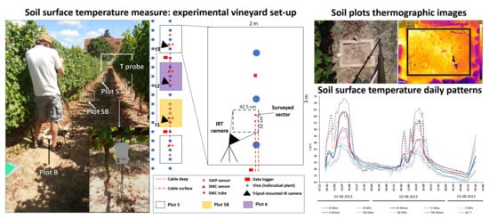
2.3. Experimental Setup
3. Results
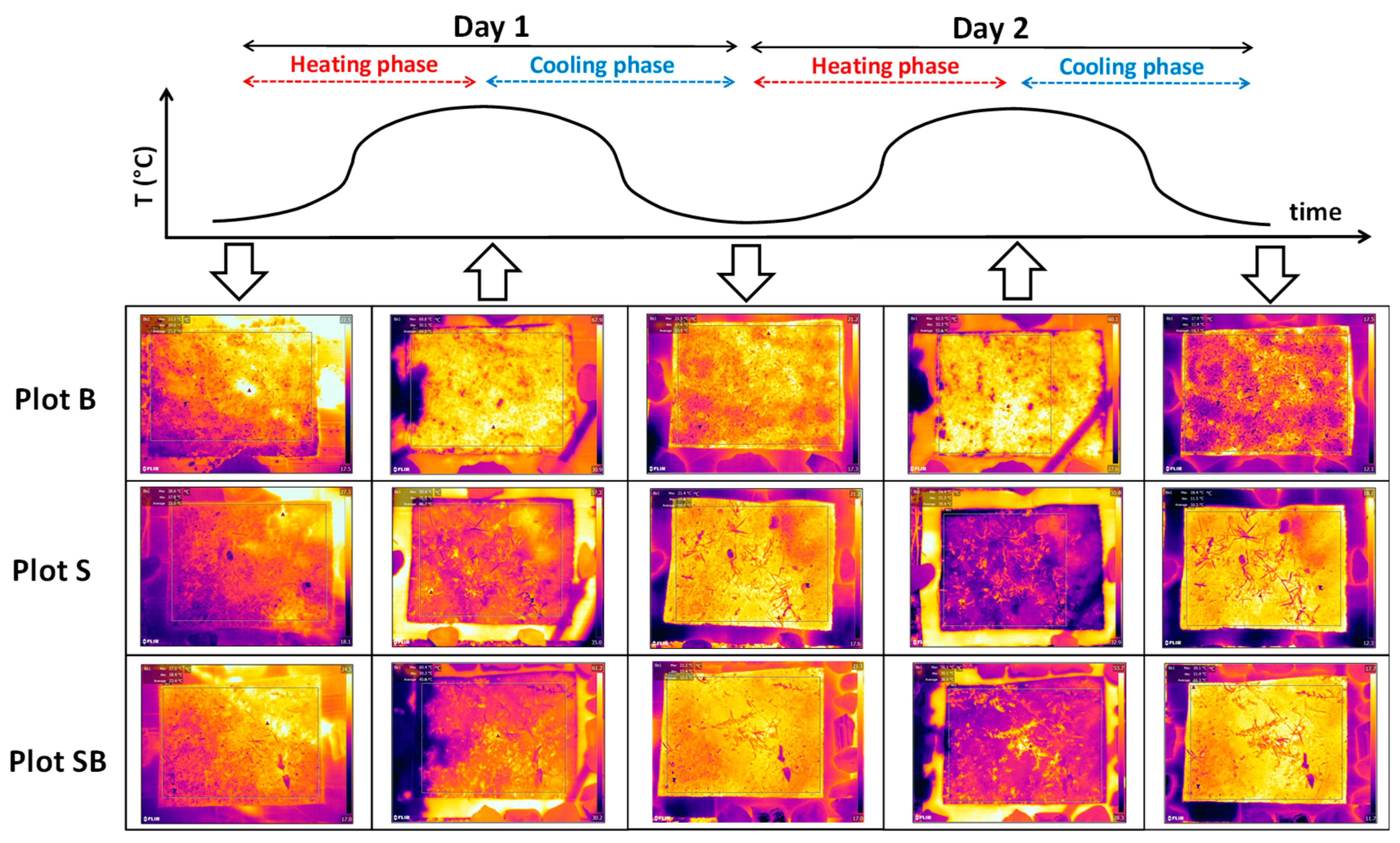
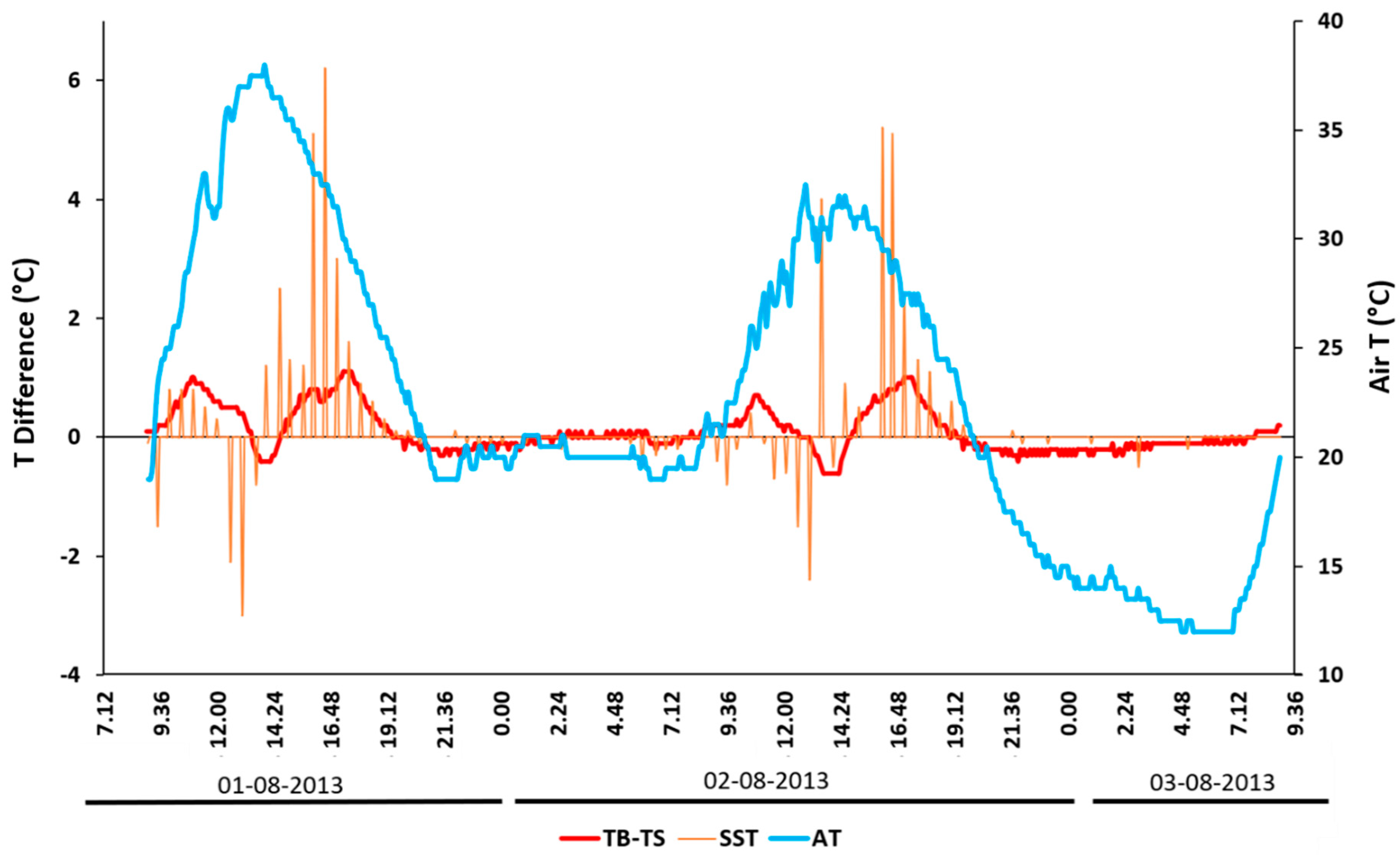
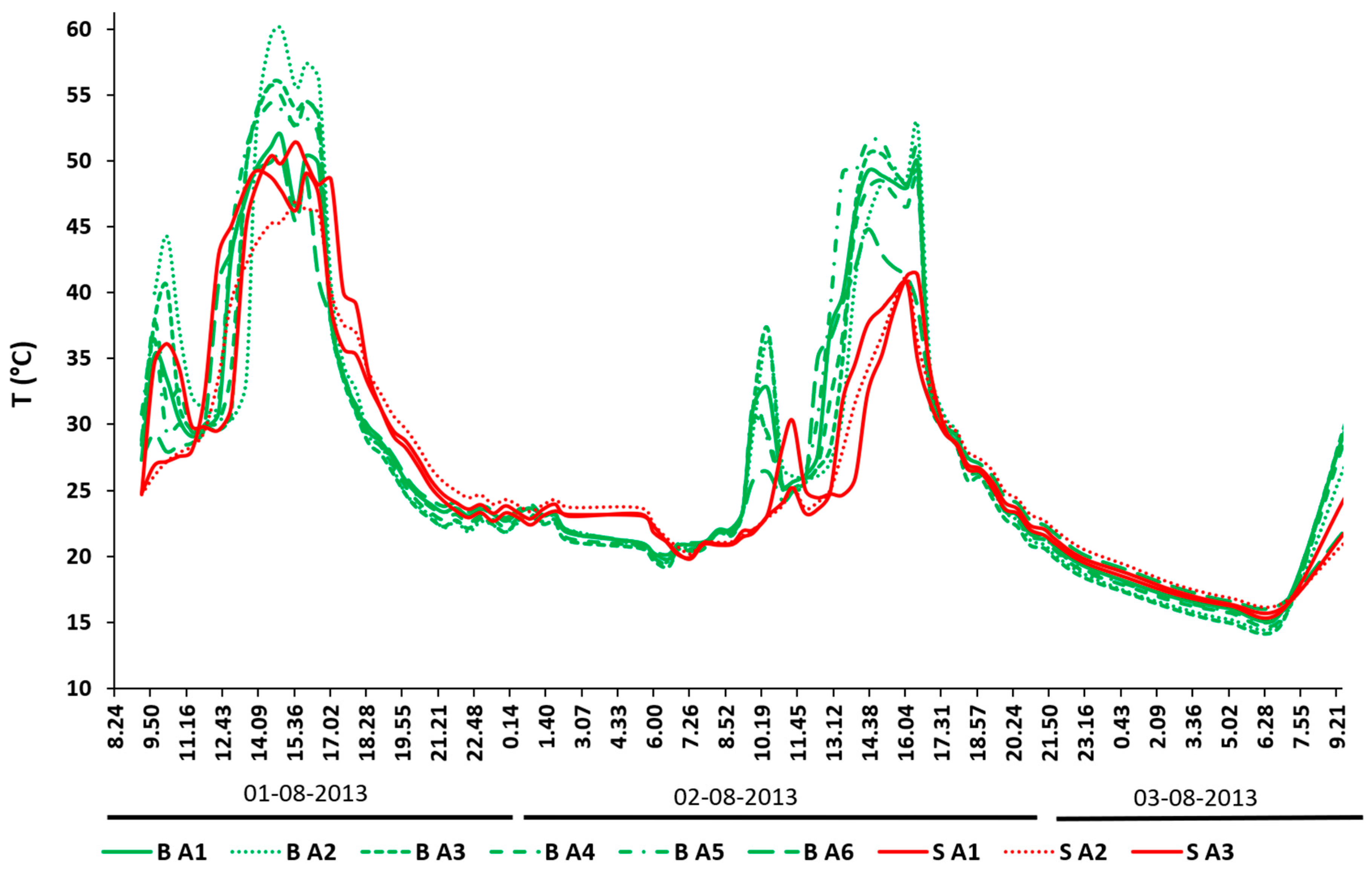
3.1. SSTs from IRTs
3.2. Soil Temperatures at a 10 cm Depth
3.3. SST Raster Analysis for a Spot in Plot SB
4. Discussion
5. Conclusions
Author Contributions
Funding
Acknowledgments
Conflicts of Interest
References
- Van De Griend, A.A.; Owe, M. On the relationship between thermal emissivity and the normalized difference vegetation index for natural surfaces. Int. J. Remote Sens. 1993, 14, 1119–1131. [Google Scholar] [CrossRef]
- Bastiaanssen, W.; Pelgrum, H.; Wang, J.; Ma, Y.; Moreno, J.; Roerink, G.; Van Der Wal, T. A remote sensing surface energy balance algorithm for land (SEBAL). J. Hydrol. 1998, 212, 213–229. [Google Scholar] [CrossRef]
- Heusinkveld, B.G.; Jacobs, A.; Holtslag, A.; Berkowicz, S. Surface energy balance closure in an arid region: Role of soil heat flux. Agric. For. Meteorol. 2004, 122, 21–37. [Google Scholar] [CrossRef]
- Niu, G.-Y.; Yang, Z.; Mitchell, K.E.; Chen, F.; Ek, M.B.; Barlage, M.; Kumar, A.; Manning, K.; Niyogi, D.; Rosero, E.; et al. The community Noah land surface model with multiparameterization options (Noah-MP): 1. Model description and evaluation with local-scale measurements. J. Geophys. Res. Space Phys. 2011, 116, 116. [Google Scholar] [CrossRef] [Green Version]
- Sellers, P.J.; Dickinson, R.E.; Randall, D.A.; Betts, A.K.; Hall, F.G.; Berry, J.A.; Collatz, G.J.; Denning, A.S.; Mooney, H.A.; Nobre, C.A.; et al. Henderson-Sellers A. Modeling the exchanges of energy, water, and carbon between continents and the atmosphere. Science 1997, 275, 502–509. [Google Scholar] [CrossRef] [Green Version]
- Mira, M.; Valor, E.; Boluda, R.; Caselles, V.; Coll, C. Influence of soil water content on the thermal infrared emissivity of bare soils: Implication for land surface temperature determination. J. Geophys. Res. Space Phys. 2007, 112, 112. [Google Scholar] [CrossRef] [Green Version]
- Steenpass, C.; VanderBorght, J.; Herbst, M.; Šimůnek, J.; Vereecken, H. Estimating Soil Hydraulic Properties from Infrared Measurements of Soil Surface Temperatures and TDR Data. Vadose Zone J. 2010, 9, 910–924. [Google Scholar] [CrossRef] [Green Version]
- Rossel, R.V.; Webster, R. Predicting soil properties from the Australian soil visible–near infrared spectroscopic database. Eur. J. Soil Sci. 2012, 63, 848–860. [Google Scholar] [CrossRef]
- McMillin, L.M. Estimation of sea surface temperatures from two infrared window measurements with different absorption. J. Geophys. Res. 1975, 80, 5113–5117. [Google Scholar] [CrossRef]
- Hulley, G.C.; Hook, S.J.; Baldridge, A.M. Investigating the effects of soil moisture on thermal infrared land surface temperature and emissivity using satellite retrievals and laboratory measurements. Remote Sens. Environ. 2010, 114, 1480–1493. [Google Scholar] [CrossRef]
- Tomlinson, C.J.; Chapman, L.; Thornes, J.E.; Baker, C. Remote sensing land surface temperature for meteorology and climatology: A review. Meteorol. Appl. 2011, 18, 296–306. [Google Scholar] [CrossRef] [Green Version]
- Li, Z.L.; Tang, B.H.; Wu, H.; Ren, H.; Yan, G.; Wan, Z.; Trigo, I.F.; Sobrino, J.A. Satellite-derived land surface temperature: Current status and perspectives. Remote Sens. Environ. 2013, 131, 14–37. [Google Scholar] [CrossRef] [Green Version]
- Abrams, M.; Tsu, H.; Hulley, G.; Iwao, K.; Pieri, D.; Cudahy, T.; Kargel, J. The Advanced Spaceborne Thermal Emission and Reflection Radiometer (ASTER) after fifteen years: Review of global products. Int. J. Appl. Earth Obs. Geoinf. 2015, 38, 292–301. [Google Scholar] [CrossRef]
- Anderson, J.M.; Wilson, S.B. The physical basis of current infrared remote-sensing techniques and the interpretation of data from aerial surveys. Int. J. Remote Sens. 1984, 5, 1–18. [Google Scholar]
- Kirkland, L.; Herr, K.; Keim, E.; Adams, P.; Salisbury, J.; Hackwell, J.; Treiman, A. First use of an airborne thermal infrared hyperspectral scanner for compositional mapping. Remote Sens. Environ. 2002, 80, 447–459. [Google Scholar] [CrossRef] [Green Version]
- Sobrino, J.A.; Jiménez-Muñoz, J.-C.; Zarco-Tejada, P.J.; Sepulcre-Canto, G.; De Miguel, E. Land surface temperature derived from airborne hyperspectral scanner thermal infrared data. Remote. Sens. Environ. 2006, 102, 99–115. [Google Scholar] [CrossRef]
- Eccel, E.; Arman, G.; Zottele, F.; Gioli, B. Thermal infrared remote sensing for high resolution minimum temperature mapping. Ital. J. Agrometeorol. 2008, 13, 52–61. [Google Scholar]
- Pasquier, C.; Bourennane, H.; Cousin, I.; Séger, M.; Dabas, M.; Thiesson, J. Comparison between thermal airborne remote sensing, multi-depth electrical resistivity profiling, and soil mapping: An example from Beauce (Loiret, France). Near Surf. Geophys. 2016, 14, 345–356. [Google Scholar] [CrossRef] [Green Version]
- Kant, Y.; Badarinath, K.V.S. Ground-based method for measuring thermal infrared effective emissivities: Implications and perspectives on the measurement of land surface temperature from satellite data. Int. J. Remote Sens. 2002, 23, 2179–2191. [Google Scholar] [CrossRef]
- Qin, Z.; Berliner, P.; Karnieli, A. Ground temperature measurement and emissivity determination to understand the thermal anomaly and its significance on the development of an arid environmental ecosystem in the sand dunes across the Israel–Egypt border. J. Arid. Environ. 2005, 60, 27–52. [Google Scholar]
- Pfister, L.; McDonnell, J.J.; Hissler, C.; Hoffmann, L. Ground-based thermal imagery as a simple, practical tool for mapping saturated area connectivity and dynamics. Hydrol. Process. 2010, 24, 3123–3132. [Google Scholar] [CrossRef]
- Price, J.C. The potential of remotely sensed thermal infrared data to infer surface soil moisture and evaporation. Water Resour. Res. 1980, 16, 787–795. [Google Scholar] [CrossRef]
- Casagli, N.; Frodella, W.; Morelli, S.; Tofani, V.; Ciampalini, A.; Intrieri, E.; Raspini, F.; Rossi, G.; Tanteri, L.; Lu, P. Spaceborne, UAV and ground-based remote sensing techniques for landslide mapping, monitoring and early warning. Geoenviron. Disasters 2017, 4, 9. [Google Scholar] [CrossRef]
- Di Traglia, F.; Nolesini, T.; Ciampalini, A.; Solari, L.; Frodella, W.; Bellotti, F.; Fumagalli, A.; De Rosa, G.; Casagli, N. Tracking morphological changes and slope instability using space-borne and ground-based SAR data. Geomorphology 2018, 300, 95–112. [Google Scholar] [CrossRef]
- Moran, M.S.; Peters-Lidard, C.D.; Watts, J.M.; McElroy, S. Estimating soil moisture at the watershed scale with satellite-based radar and land surface models. Can. J. Remote Sens. 2004, 30, 805–826. [Google Scholar] [CrossRef] [Green Version]
- Coolbaugh, M.F.; Kratt, C.; Fallacaro, A.; Calvin, W.M.; Taranik, J.V. Detection of geothermal anomalies using advanced spaceborne thermal emission and reflection radiometer (ASTER) thermal infrared images at Bradys Hot Springs, Nevada, USA. Remote Sens. Environ. 2007, 106, 350–359. [Google Scholar] [CrossRef]
- Gigli, G.; Frodella, W.; Garfagnoli, F.; Morelli, S.; Mugnai, F.; Menna, F.; Casagli, N. 3-D geomechanical rock mass characterization for the evaluation of rockslide susceptibility scenarios. Landslides 2014, 11, 131–140. [Google Scholar] [CrossRef]
- Kerr, Y.H.; Lagouarde, J.P.; Imbernon, J. Accurate land surface temperature retrieval from AVHRR data with use of an improved split window algorithm. Remote Sens. Environ. 1992, 41, 197–209. [Google Scholar] [CrossRef]
- Prata, A.J.; Caselles, V.; Coll, C.; Sobrino, J.A.; Ottle, C. Thermal remote sensing of land surface temperature from satellites: Current status and future prospects. Remote Sens. Rev. 1995, 12, 175–224. [Google Scholar] [CrossRef]
- Wan, Z.; Zhang, Y.; Zhang, Q.; Li, Z.L. Validation of the land-surface temperature products retrieved from Terra Moderate Resolution Imaging Spectroradiometer data. Remote Sens. Environ. 2002, 83, 163–180. [Google Scholar] [CrossRef]
- Zhou, D.K.; Larar, A.M.; Liu, X. On the relationship between land surface infrared emissivity and soil moisture. J. Appl. Remote Sens. 2018, 12, 016030. [Google Scholar] [CrossRef] [Green Version]
- Shaver, G.R.; Canadell, J.; Chapin, F.S.; Gurevitch, J.; Harte, J.; Henry, G.; Ineson, P.; Jonasson, S.; Melillo, J.; Pitelka, L.; et al. Global Warming and Terrestrial Ecosystems: A Conceptual Framework for Analysis: Ecosystem responses to global warming will be complex and varied. Ecosystem warming experiments hold great potential for providing insights on ways terrestrial ecosystems will respond to upcoming decades of climate change. Documentation of initial conditions provides the context for understanding and predicting ecosystem responses. Aibs Bull. 2000, 50, 871–882. [Google Scholar]
- Lindner, M.; Maroschek, M.; Netherer, S.; Kremer, A.; Barbati, A.; Garcia-Gonzalo, J.; Seidl, R.; Delzon, S.; Corona, P.; Kolström, M.; et al. Climate change impacts, adaptive capacity, and vulnerability of European forest ecosystems. For. Ecol. Manag. 2010, 259, 698–709. [Google Scholar] [CrossRef]
- Meola, C.; Boccardi, S.; Carlomagno, G.M. Infrared Thermography in the Evaluation of Aerospace Composite Materials: Infrared Thermography to Composites; Woodhead Publishing: Cambridge, UK, 2016; pp. 57–83. [Google Scholar] [CrossRef]
- Jones, H.G.; Leinonen, I. Thermal imaging for the study of plant water relations. J. Agric. Meteorol. 2003, 59, 205–217. [Google Scholar] [CrossRef] [Green Version]
- Grant, O.M.; Tronina, Ł.; Jones, H.G.; Chaves, M.M. Exploring thermal imaging variables for the detection of stress responses in grapevine under different irrigation regimes. J. Exp. Bot. 2006, 58, 815–825. [Google Scholar] [CrossRef]
- Spampinato, L.; Calvari, S.; Oppenheimer, C.; Boschi, E. Volcano surveillance using infrared cameras. Earth Sci. Rev. 2011, 106, 63–91. [Google Scholar] [CrossRef]
- Reinert, S.; Bögelein, R.; Thomas, F.M. Use of thermal imaging to determine leaf conductance along a canopy gradient in European beech (Fagus sylvatica). Tree Physiol. 2012, 32, 294–302. [Google Scholar] [CrossRef] [Green Version]
- Clark, M.R.; McCann, D.M.; Forde, M.C. Application of infrared thermography to the non-destructive testing of concrete and masonry bridges. NDT Int. 2003, 36, 265–275. [Google Scholar] [CrossRef]
- De Lima, J.L.M.P.; Abrantes, J.R.C.B. Can infrared thermography be used to estimate soil surface microrelief and rill morphology? Catena 2014, 113, 314–322. [Google Scholar] [CrossRef]
- Frodella, W.; Gigli, G.; Morelli, S.; Lombardi, L.; Casagli, N. Landslide Mapping and Characterization through Infrared Thermography (IRT): Suggestions for a Methodological Approach from Some Case Studies. Remote Sens. 2017, 9, 1281. [Google Scholar] [CrossRef] [Green Version]
- Nolesini, T.; Frodella, W.; Bianchini, S.; Casagli, N. Detecting Slope and Urban Potential Unstable Areas by Means of Multi-Platform Remote Sensing Techniques: The Volterra (Italy) Case Study. Remote Sens. 2016, 8, 746. [Google Scholar] [CrossRef] [Green Version]
- Di Traglia, F.; Nolesini, T.; Solari, L.; Ciampalini, A.; Frodella, W.; Steri, D.; Allotta, B.; Rindi, A.; Marini, L.; Monni, N.; et al. Lava delta deformation as a proxy for submarine slope instability. Earth Planet. Sci. Lett. 2018, 488, 46–58. [Google Scholar] [CrossRef]
- Frodella, W.; Morelli, S.; Pazzi, V. Infrared Thermographic surveys for landslide mapping and characterization: The Rotolon DSGSD (Norther Italy) case study. Ital. J. Eng. Geol. Environ. 2017, 2017. [Google Scholar] [CrossRef]
- Maldague, X. Theory and Practice of Infrared Technology for Non-Destructive Testing; John-Wiley & Sons: Hoboken, NJ, USA, 2001; 684p. [Google Scholar]
- Baldock, J.A.; Smernik, R.J. Chemical composition and bioavailability of thermally altered Pinus resinosa (Red pine) wood. Org. Geochem. 2002, 33, 1093–1109. [Google Scholar] [CrossRef]
- Verheijen, F.G.; Montanarella, L.; Bastos, A.C. Sustainability, certification, and regulation of biochar. Pesqui. Agropecuária Bras. 2012, 47, 649–653. [Google Scholar] [CrossRef] [Green Version]
- Jeffery, S.; Verheijen, F.G.; van der Velde, M.; Bastos, A.C. A quantitative review of the effects of biochar application to soils on crop productivity using meta-analysis. Agric. Ecosyst. Environ. 2011, 144, 175–187. [Google Scholar] [CrossRef]
- Jeffery, S.; Verheijen, F.G.; Bastos, A.C.; Van Der Velde, M. A comment on ‘Biochar and its effects on plant productivity and nutrient cycling: A meta-analysis’: On the importance of accurate reporting in supporting a fast-moving research field with policy implications. Gcb Bioenergy 2014, 6, 176–179. [Google Scholar] [CrossRef] [Green Version]
- Jeffery, S.; Abalos, D.; Prodana, M.; Bastos, A.C.; Van Groenigen, J.W.; Hungate, B.A.; Verheijen, F. Biochar boosts tropical but not temperate crop yields. Environ. Res. Lett. 2017, 12, 053001. [Google Scholar] [CrossRef]
- Jeffery, S.; Verheijen, F.G.; Kammann, C.; Abalos, D. Biochar effects on methane emissions from soils: A meta-analysis. Soil Biol. Biochem. 2016, 101, 251–258. [Google Scholar] [CrossRef]
- Cayuela, M.L.; Van Zwieten, L.; Singh, B.P.; Jeffery, S.; Roig, A.; Sánchez-Monedero, M.A. Biochar’s role in mitigating soil nitrous oxide emissions: A review and meta-analysis. Agric. Ecosyst. Environ. 2014, 191, 5–16. [Google Scholar] [CrossRef]
- Wang, J.; Xiong, Z.; Kuzyakov, Y. Biochar stability in soil: Meta-analysis of decomposition and priming effects. GCB Bioenergy 2016, 8, 512–523. [Google Scholar] [CrossRef] [Green Version]
- Omondi, M.O.; Xia, X.; Nahayo, A.; Liu, X.; Korai, P.K.; Pan, G. Quantification of biochar effects on soil hydrological properties using meta-analysis of literature data. Geoderma 2016, 274, 28–34. [Google Scholar] [CrossRef]
- Verheijen, F.G.A.; Zhuravel, A.; Silva, F.; Amaro, A.; Ben-Hur, M.; Keizer, J.J. The influence of biochar particle size and concentration on bulk density and maximum water holding capacity of sandy vs. sandy loam soil in a column experiment. Geoderma 2019, 347, 194–202. [Google Scholar] [CrossRef]
- Abrol, V.; Ben-Hur, M.; Verheijen, F.G.; Keizer, J.J.; Martins, M.A.; Tenaw, H.; Tchehansky, L.; Graber, E.R. Biochar effects on soil water infiltration and erosion under seal formation conditions: Rainfall simulation experiment. J. Soils Sediments 2016, 16, 2709–2719. [Google Scholar] [CrossRef]
- Hilber, I.; Bastos, A.C.; Loureiro, S.; Soja, G.; Marsz, A.; Cornelissen, G.; Bucheli, T.D. The different faces of biochar: Contamination risk versus remediation tool. J. Environ. Eng. Landsc. Manag. 2017, 25, 86–104. [Google Scholar] [CrossRef] [Green Version]
- Davidson, E.A.; Janssens, I.A. Temperature sensitivity of soil carbon decomposition and feedbacks to climate change. Nature 2006, 440, 165–173. [Google Scholar] [CrossRef]
- Intergovernmental Panel on Climate Change. Climate Change 2014—Impacts, Adaptation and Vulnerability: Regional Aspects; Cambridge University Press: Cambridge, UK, 2014. [Google Scholar]
- Routson, C.C.; McKay, N.P.; Kaufman, D.S.; Erb, M.P.; Goosse, H.; Shuman, B.N.; Rodysill, J.R.; Ault, T. Mid-latitude net precipitation decreased with Arctic warming during the Holocene. Nature 2019, 568, 83–87. [Google Scholar] [CrossRef]
- Verheijen, F.G.; Jeffery, S.; Van Der Velde, M.; Penížek, V.; Béland, M.; Bastos, A.C.; Keizer, J.J. Reductions in soil surface albedo as a function of biochar application rate: Implications for global radiative forcing. Environ. Res. Lett. 2013, 8, 044008. [Google Scholar] [CrossRef] [Green Version]
- Nelissen, V.; Ruysschaert, G.; Manka’Abusi, D.; D’Hose, T.; De Beuf, K.; Al-Barri, B.; Boeckx, P. Impact of a woody biochar on properties of a sandy loam soil and spring barley during a two-year field experiment. Eur. J. Agron. 2015, 62, 65–78. [Google Scholar] [CrossRef]
- Ventura, M.; Sorrenti, G.; Panzacchi, P.; George, E.; Tonon, G. Biochar Reduces Short-Term Nitrate Leaching from A Horizon in an Apple Orchard. J. Environ. Qual. 2013, 42, 76–82. [Google Scholar] [CrossRef]
- Usowicz, B.; Lipiec, J.; Łukowski, M.; Marczewski, W.; Usowicz, J. The effect of biochar application on thermal properties and albedo of loess soil under grassland and fallow. Soil Tillage Res. 2016, 164, 45–51. [Google Scholar] [CrossRef]
- Tammeorg, P.; Bastos, A.C.; Jeffery, S.; Rees, F.; Kern, J.; Graber, E.R.; Cordovil, C.M.D.S. Biochars in soils: Towards the required level of scientific understanding. J. Environ. Eng. Landsc. Manag. 2017, 25, 192–207. [Google Scholar] [CrossRef] [Green Version]
- Lillesand, T.M.; Kiefer, R.W.; Chipman, J.W. Remote Sensing and Image Interpretation, 6th ed.; John Wiley and Sons, Inc.: Hoboken, NJ, USA, 2008. [Google Scholar]
- Dhar, N.K.; Sood, A.K.; Dat, R. Advances in Infrared Detector Array Technology. In Optoelectronics—Advanced Materials and Devices; INTECH Open Access Publisher: London, UK, 2013; Volume 1. [Google Scholar]
- FLIR Systems Inc. ThermaCAM SC620 Technical Specifications. 2009. Available online: http://www.flir.com/cs/emea/en/view/?id=41965 (accessed on 21 January 2020).
- FLIR Systems Inc. FLIR Tools+ Datasheet. 2015. Available online: https://www.infraredcamerawarehouse.com/content/FLIR%20Datasheets/FLIR%20ToolsPlus%20Datasheet.pdf (accessed on 22 January 2020).
- Incropera, P.F.; De Witt, D.P. Introduction to Heat Transfer; John Wiley: Hobekone, NJ, USA, 1985; pp. 654–746. [Google Scholar]
- Rees, W.G. Physical Principles of Remote Sensing, 2nd ed.; Cambridge University Press: Cambridge, UK, 2001. [Google Scholar]
- Gupta, R.P. Interpretation of data in the thermal-infrared region. In Remote Sensing Geology; Springer: New York, NY, USA, 2003; pp. 190–203. [Google Scholar]
- Verstraeten, W.W.; Veroustraete, F.; van der Sande, C.J.; Grootaers, I.; Feyen, J. Soil moisture retrieval using thermal inertia, determined with visible and thermal spaceborne data, validated for European forests. Remote Sens. Environ. 2006, 101, 299–314. [Google Scholar] [CrossRef]
- Hardgrove, C.; Moersch, J.; Whisner, S. Thermal imaging of sedimentary features on alluvial fans. Planet. Space Sci. 2010, 58, 482–508. [Google Scholar] [CrossRef]
- Van de Griend, A.A.; Camillo, P.J.; Gurney, R.J. Discrimination of soil physical parameters, thermal inertia, and soil moisture from diurnal surface temperature fluctuations. Water Resour. Res. 1985, 21, 997–1009. [Google Scholar] [CrossRef]
- Jakosky, B.M. On the thermal properties of Martian fines. Icarus 1986, 66, 117–124. [Google Scholar] [CrossRef]
- Mutlutürk, M.; Altindag, R.; Türk, G. A decay function model for the integrity loss of rock when subjected to recurrent cycles of freezing–thawing and heating–cooling. Int. J. Rock Mech. Min. Sci. 2004, 41, 237–244. [Google Scholar] [CrossRef]
- Ball, M.; Pinkerton, H. Factors affecting the accuracy of thermal imaging cameras in volcanology. J. Geophys. Res. 2006, 111, B11203. [Google Scholar] [CrossRef]
- Salisbury, J.W.; D’Aria, D.M. Emissivity of terrestrial materials in the 8–14 µm atmospheric window. Remote Sens. Environ. 1992, 42, 83–106. [Google Scholar] [CrossRef]
- Rubio, E.; Caselles, V.; Badenas, C. Emissivity measurements of several soils and vegetation types in the 8–14 μm wave band: Analysis of two field methods. Remote Sens. Environ. 1997, 59, 490–521. [Google Scholar] [CrossRef]
- Garrity, D.; Bindraban, P. A Globally Distributed Soil Spectral Library Visible near Infrared Diffuse Reflectance Spectra; ICRAF (World Agroforestry Centre)/ISRIC (World Soil Information) Spectral Library: Nairobi, Kenya, 2004. [Google Scholar]
- ISO 18434-1:2008 Condition Monitoring and Diagnostics of Machines—Thermography—Part 1: General Procedures. Available online: https://www.iso.org/standard/41648.html (accessed on 18 January 2019).
- Avdelidis, N.P.; Moropoulou, A. Emissivity considerations in building thermography. Energy Build. 2003, 35, 663–667. [Google Scholar] [CrossRef]
- Chicco, J.M.; Vacha, D.; Mandrone, G. Thermo-Physical and Geo-Mechanical Characterization of Faulted Carbonate Rock Masses (Valdieri, Italy). Remote Sens. 2019, 11, 179. [Google Scholar] [CrossRef] [Green Version]
- Metzger, M.J.; Bunce, R.G.H.; Jongman, R.H.G.; Sayre, R.; Trabucco, A.; Zomer, R. A high-resolution bioclimate map of the world: A unifying framework for global biodiversity research and monitoring. Glob. Ecol. Biogeogr. 2013, 22, 630–638. [Google Scholar] [CrossRef] [Green Version]
- Pereira, V.; FitzPatrick, E.A. Cambisols and related soils in north-central Portugal: Their genesis and classification. Geoderma 1995, 66, 185–212. [Google Scholar] [CrossRef]
- Inácio, M.; Pereira, V.; Pinto, M. The soil geochemical atlas of Portugal: Overview and applications. J. Geochem. Explor. 2008, 98, 22–33. [Google Scholar] [CrossRef]
- King, P.M. Comparison of methods for measuring severity of water repellence of sandy soils and assesment of some factors that affect its measurement (Australia). Aust. J. Soil Res. 1981, 19, 275–285. [Google Scholar] [CrossRef]
- Keizer, J.J.; Doerr, S.H.; Malvar, M.C.; Ferreira, A.J.D.; Pereira, V.M.F.G. Temporal and spatial variations in topsoil water repellency throughout a crop-rotation cycle on sandy soil in north-central Portugal. Hydrol. Process. 2007, 21, 2317–2324. [Google Scholar] [CrossRef]
- Prodana, M.; Bastos, A.C.; Amaro, A.; Cardoso, D.; Morgado, R.; Machado, A.L.; Loureiro, S. Biomonitoring tools for biochar and biochar-compost amended soil under viticulture: Looking at exposure and effects. Appl. Soil Ecol. 2019, 137, 120–128. [Google Scholar] [CrossRef]
- IPMA (Instituto Português do Mar e da Atmosfera). Available online: https://www.ipma.pt/pt/index.html (accessed on 21 January 2020).
- FLIR Systems Inc. ThermaCAM SC620 User’s Manual; FLIR Systems Inc.: Wilsonville, OR, USA, 2009. [Google Scholar]
- Rossel, R.A.V.; Behrens, T.; Ben-Dor, E.; Brown, D.; Demattê, J.; Shepherd, K.; Shi, Z.; Stenberg, B.; Stevens, A.; Adamchuk, V.; et al. A global spectral library to characterize the world’s soil. Earth-Science Rev. 2016, 155, 198–230. [Google Scholar] [CrossRef] [Green Version]
- Salazar, R.K.; Laurente, C.L.B. Emissivity of “Grey” Bodies, Surface Roughness and other Measures. Recoletos Multidiscip. Res. J. 2014, 2, 2. [Google Scholar]
- Lou, C.W.; Lin, J.H. Evaluation of bamboo charcoal/stainless steel/TPU composite woven fabrics. Fibers Polym. 2011, 12, 514. [Google Scholar] [CrossRef]
- ESRI ArcGis Raster Calculator ArcMap 10.3.2. Available online: http://desktop.arcgis.com/en/arcmap/10.3/tools/spatial-analyst-toolbox/raster-calculator.htm (accessed on 23 February 2020).
- De Lima, J.L.M.P.; Abrantes, J.R.C.B.; Silva, V.P., Jr.; Montenegro, A.A.A. Prediction of skin surface soil permeability by infrared thermography: A soil flume experiment. Quant. Infrared Thermogr. J. 2014, 11, 161–169. [Google Scholar] [CrossRef]
- De Lima, J.L.M.P.; Abrantes, J.R.C.B.; Silva, V.P., Jr.; De Lima, M.I.P.; Montenegro, A.A.A. Mapping soil surface macropores using infrared thermography: An exploratory laboratory study. Sci. World J. 2014, 2014, 84560. [Google Scholar] [CrossRef] [Green Version]
- Abrantes, J.R.C.B.; De Lima, J.L.M.P.; Prats, S.A.; Keizer, J.J. Assessing soil water repellency spatial variability using a thermographic technique: Small-scale laboratory study. Geoderma 2017, 287, 98–104. [Google Scholar] [CrossRef]
- Abrantes, J.R.C.B.; De Lima, J.L.M.P.; Prats, S.A.; Keizer, J.J. Field assessment of soil water repellency using infrared thermography. Forum Geogr. 2016, 15, 12–18. [Google Scholar] [CrossRef]
- Kirschbaum, M. The temperature dependence of soil organic matter decomposition, and the effect of global warming on soil organic C storage. Soil Biol. Biochem. 1995, 27, 753–760. [Google Scholar] [CrossRef]
- Usowicz, B.; Lipiec, J.; Lukowski, M.; Marczewski, W.; Usowicz, J. The effect of biochar application on thermal inertia of soil. EGU General Assembly Conference Abstracts. Available online: https://ui.adsabs.harvard.edu/abs/2015EGUGA..17.9373U/abstract (accessed on 25 April 2020).
- Qiu, G.Y.; Yano, T.; Momii, K. An improved methodology to measure evaporation from bare soil based on comparison of surface temperature with a dry soil surface. J. Hydrol. 1998, 210, 93–105. [Google Scholar] [CrossRef]


| Feature | Unit | Value |
|---|---|---|
| Detector size | pixel | 640 × 480 |
| Spectral range | µm | (7.5, 13) |
| Temperature range | °C | (−40, +500) |
| Thermal accuracy | °C | ±2 |
| Thermal sensitivity | mK | 40 |
| Field of view (FOV) | ° | 24 × 18 |
| Lens | ° | 24 |
| Spatial resolution | mrad | 0.65 |
| Minimum focus distance | m | 0.3 |
| Image frequency | Hz | 30 |
| Heading | 1 August | 2 August | 3 August |
|---|---|---|---|
| T med (°C) | 22.0 | 21.4 | 19.1 |
| T max (°C) | 31.9 | 28.5 | 26.6 |
| T min (°C) | 14.9 | 14.6 | 12.1 |
| RH med (%) | 75 | 75 | 75 |
| RH max (%) | 98 | 100 | 99 |
| RH min (%) | 36 | 39 | 45 |
| Daily Rainfall (mm) | 0.0 | 0.9 | 0.0 |
© 2020 by the authors. Licensee MDPI, Basel, Switzerland. This article is an open access article distributed under the terms and conditions of the Creative Commons Attribution (CC BY) license (http://creativecommons.org/licenses/by/4.0/).
Share and Cite
Frodella, W.; Lazzeri, G.; Moretti, S.; Keizer, J.; Verheijen, F.G.A. Applying Infrared Thermography to Soil Surface Temperature Monitoring: Case Study of a High-Resolution 48 h Survey in a Vineyard (Anadia, Portugal). Sensors 2020, 20, 2444. https://0-doi-org.brum.beds.ac.uk/10.3390/s20092444
Frodella W, Lazzeri G, Moretti S, Keizer J, Verheijen FGA. Applying Infrared Thermography to Soil Surface Temperature Monitoring: Case Study of a High-Resolution 48 h Survey in a Vineyard (Anadia, Portugal). Sensors. 2020; 20(9):2444. https://0-doi-org.brum.beds.ac.uk/10.3390/s20092444
Chicago/Turabian StyleFrodella, William, Giacomo Lazzeri, Sandro Moretti, Jacob Keizer, and Frank G. A. Verheijen. 2020. "Applying Infrared Thermography to Soil Surface Temperature Monitoring: Case Study of a High-Resolution 48 h Survey in a Vineyard (Anadia, Portugal)" Sensors 20, no. 9: 2444. https://0-doi-org.brum.beds.ac.uk/10.3390/s20092444