Development of Non Expensive Technologies for Precise Maneuvering of Completely Autonomous Unmanned Aerial Vehicles †


Abstract
:1. Introduction
1.1. Overview of the Project & Article Novelties
- Engines
- Flight Controller
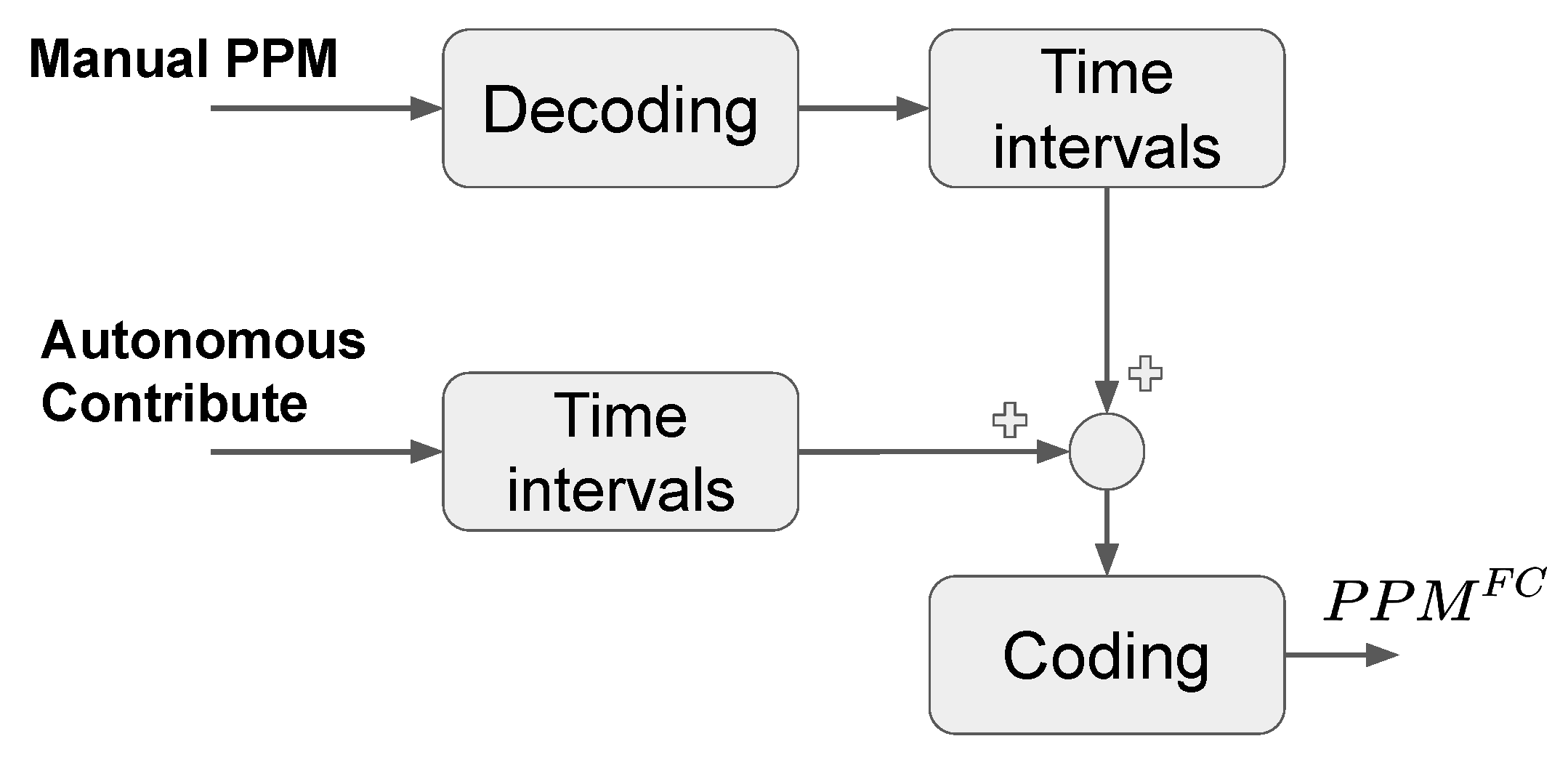
- Signal Mixer
- –
- Receiver
- *
- Human pilot
- –
- Navigation System (Cyber-pilot)
- *
- Sensors
- ·
- IMU
- ·
- Stabilized Camera
2. Hardware Architecture
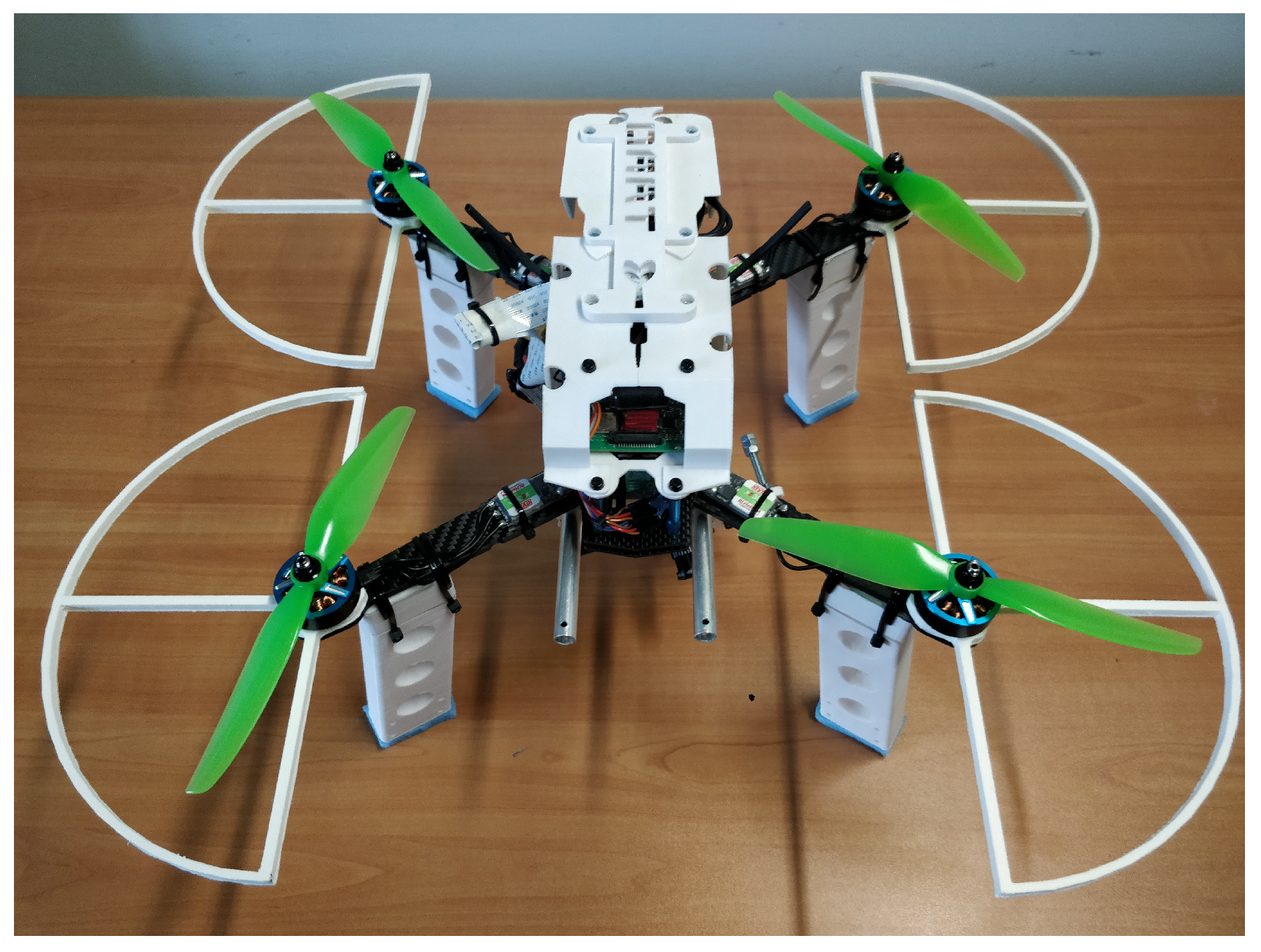
2.1. Mechanical Structure
2.2. Hardware Configuration
2.3. Sensors Units
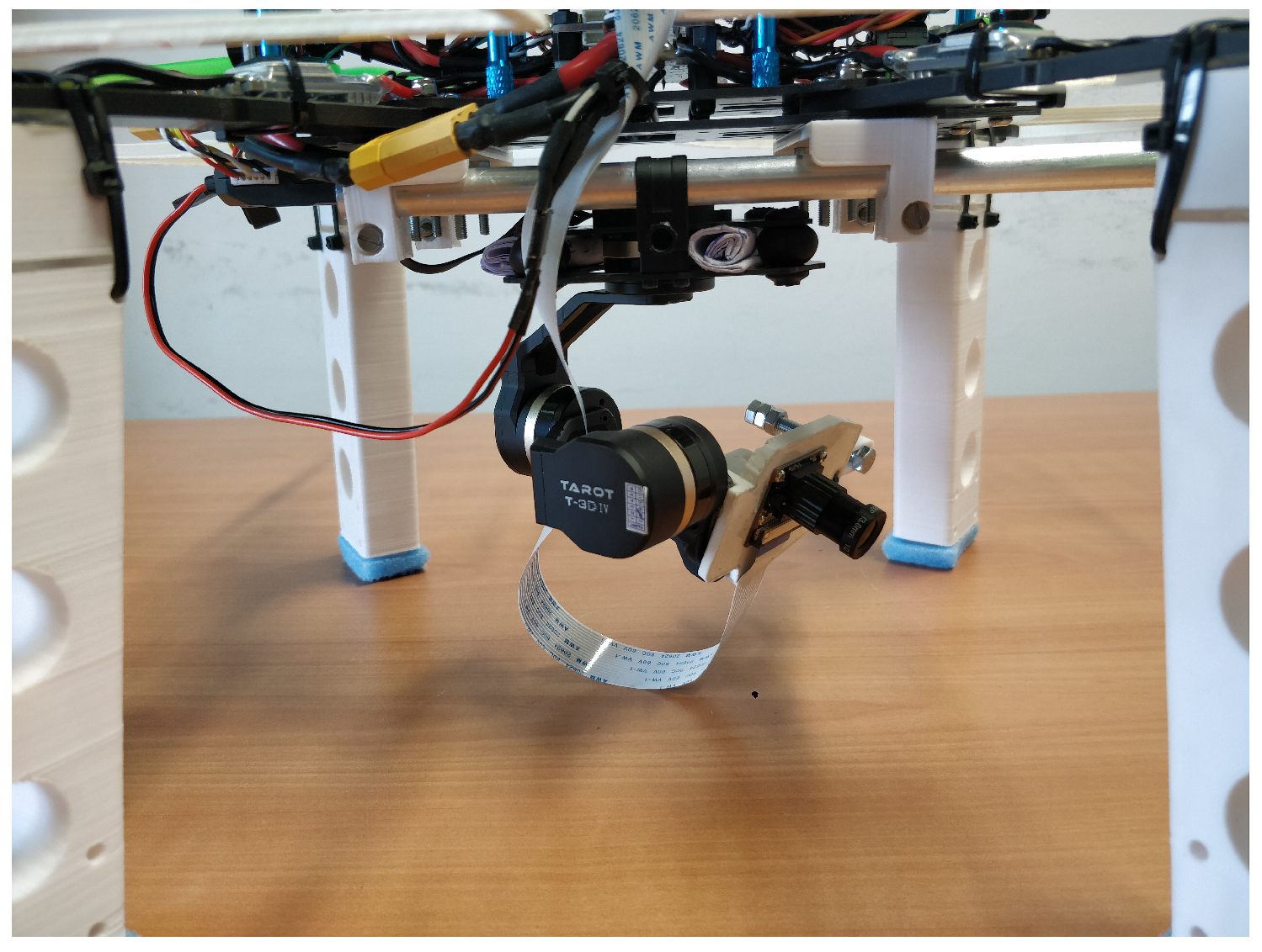
2.4. Gimbal Suspension
3. Software Modules
3.1. Low-Level Module: Internal Control of the System Attitude
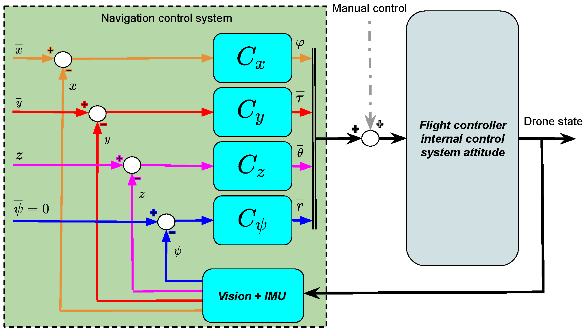
3.2. High-Level Module: Autonomous Navigation System
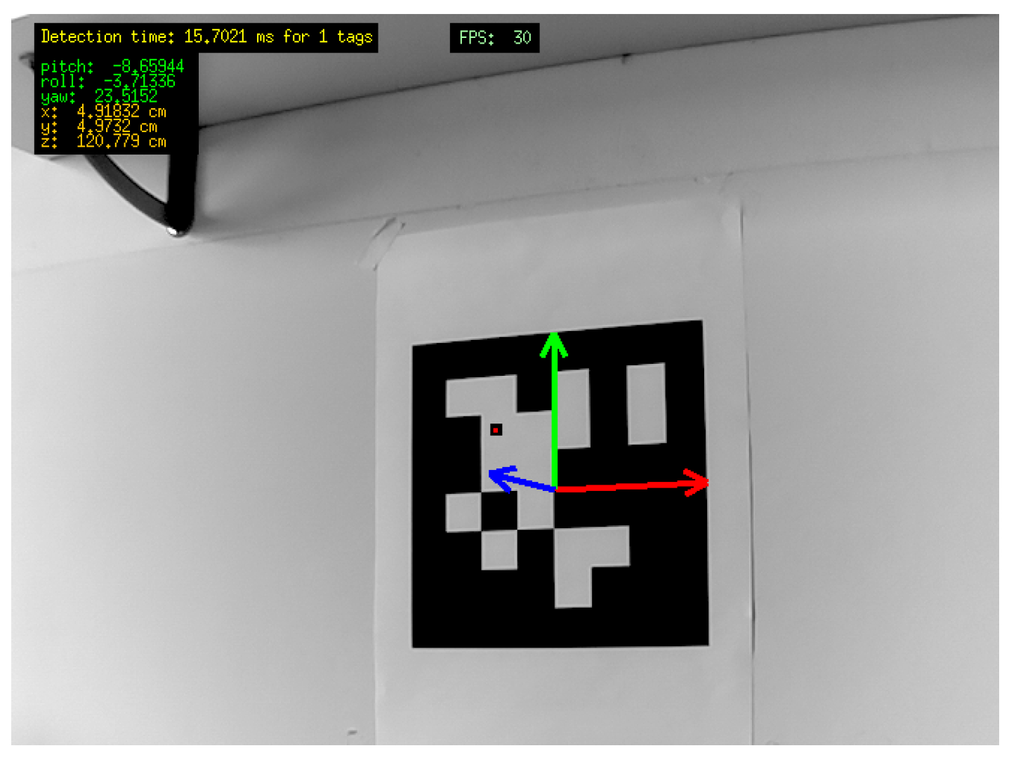
3.2.1. Computer Vision System
3.2.2. PID-Based Control System
3.2.3. Madgwick Sensor Fusion Filter
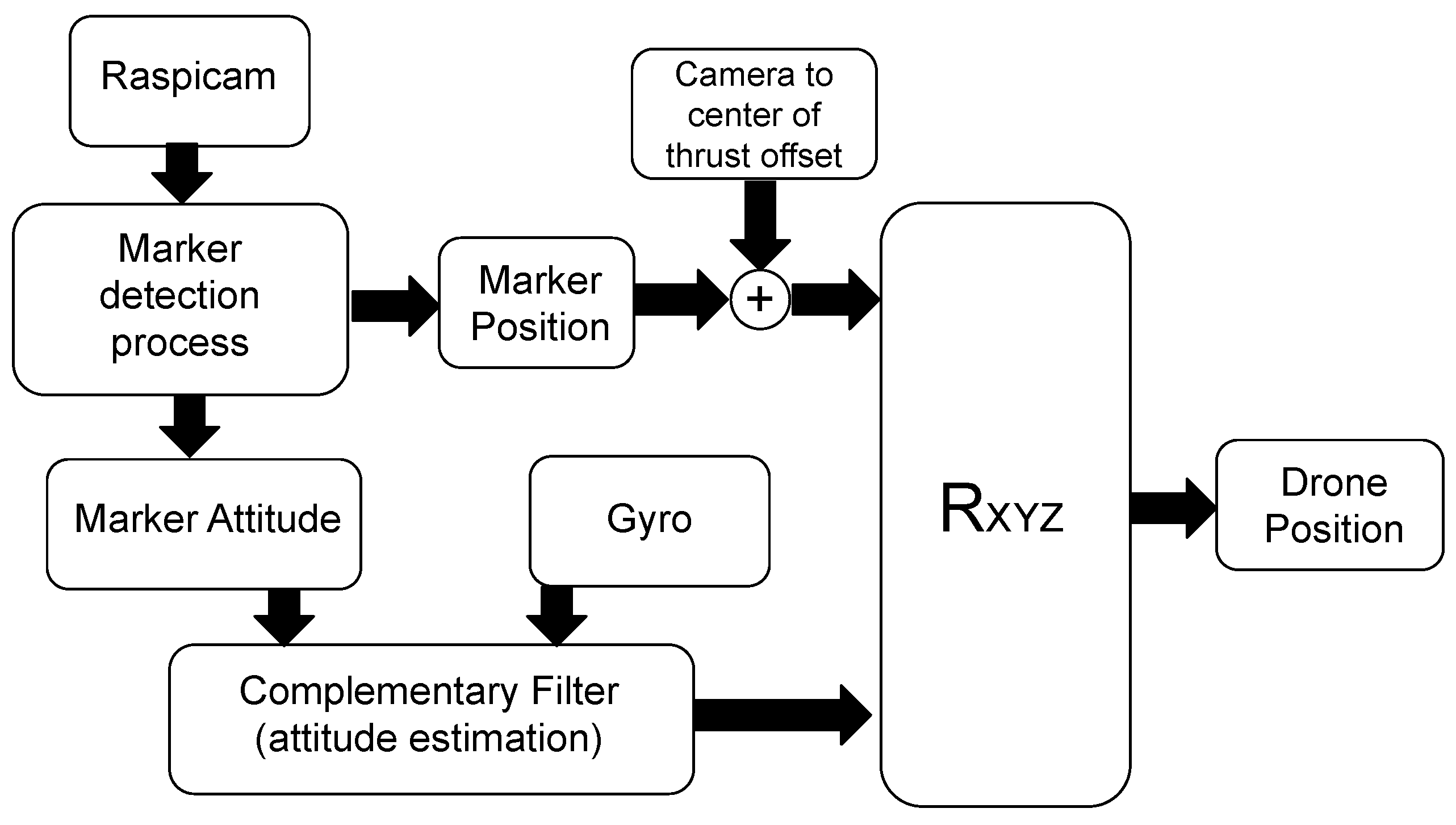
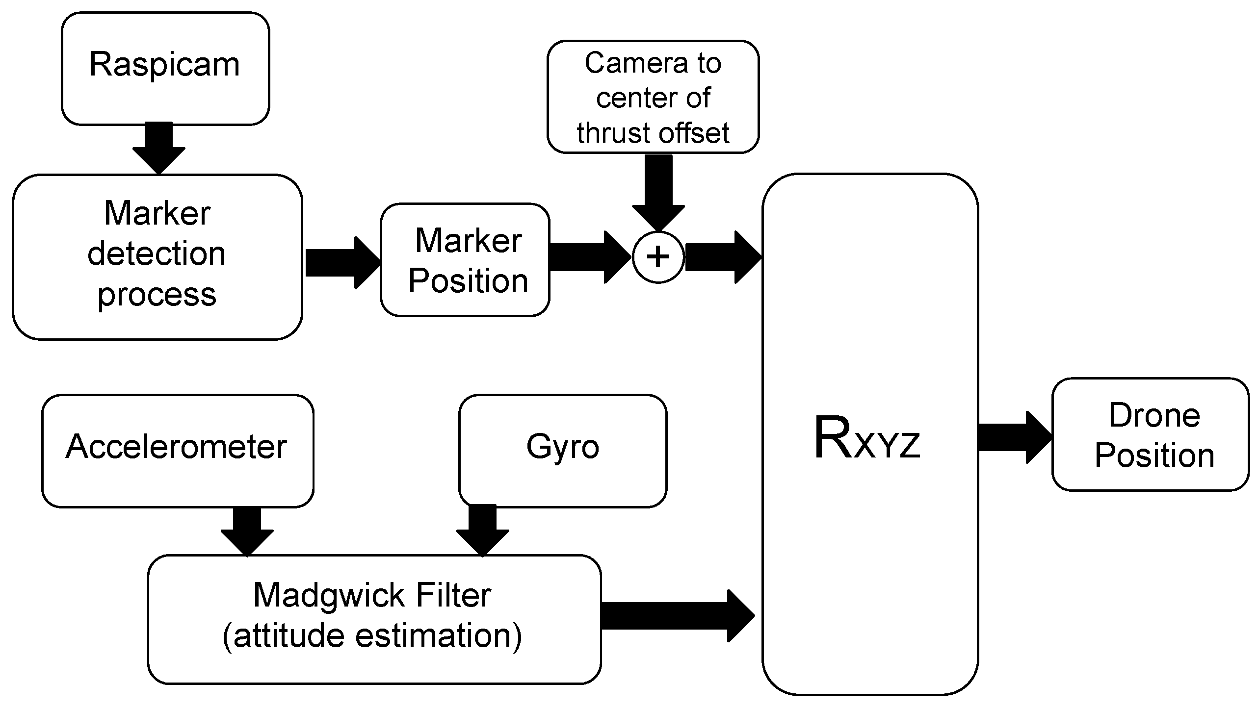
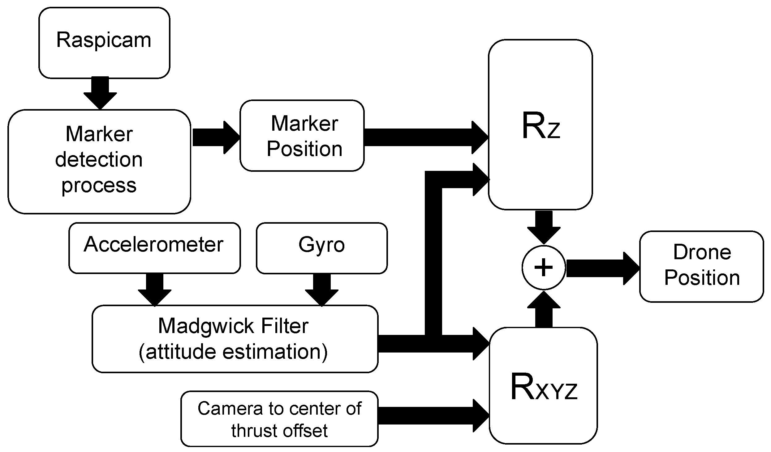
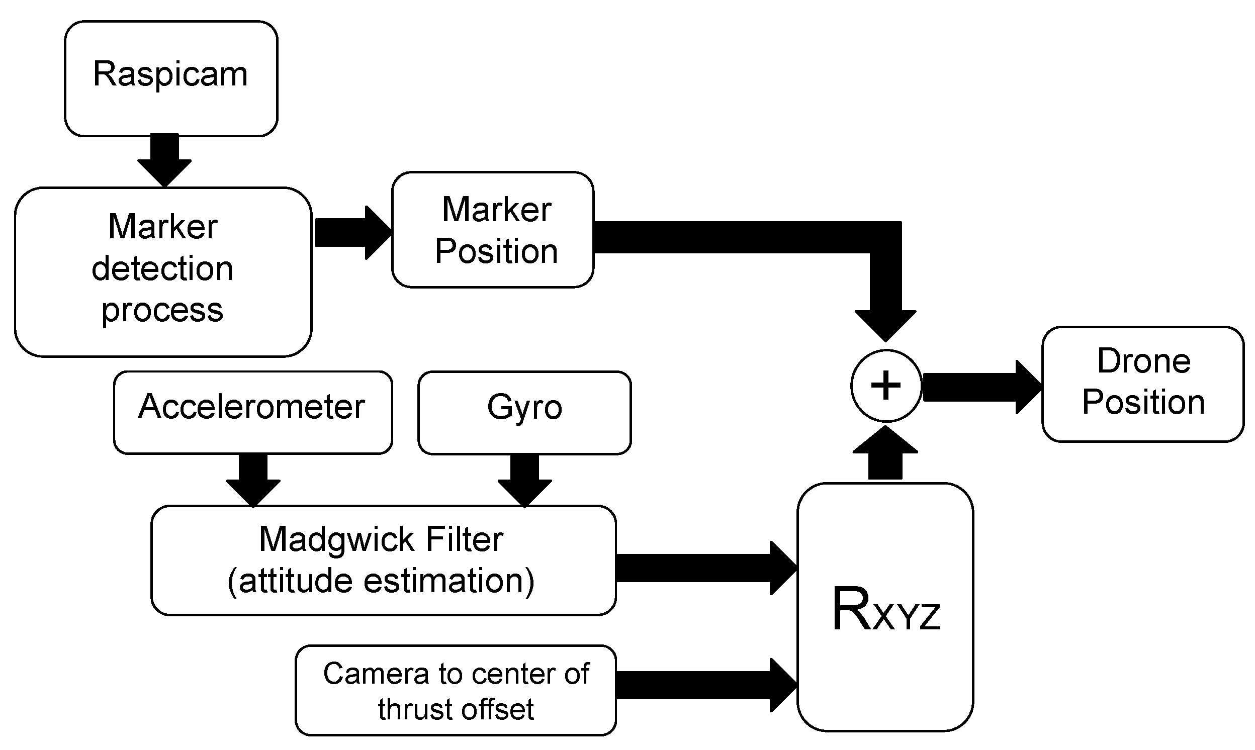
3.2.4. Position Estimation Methods
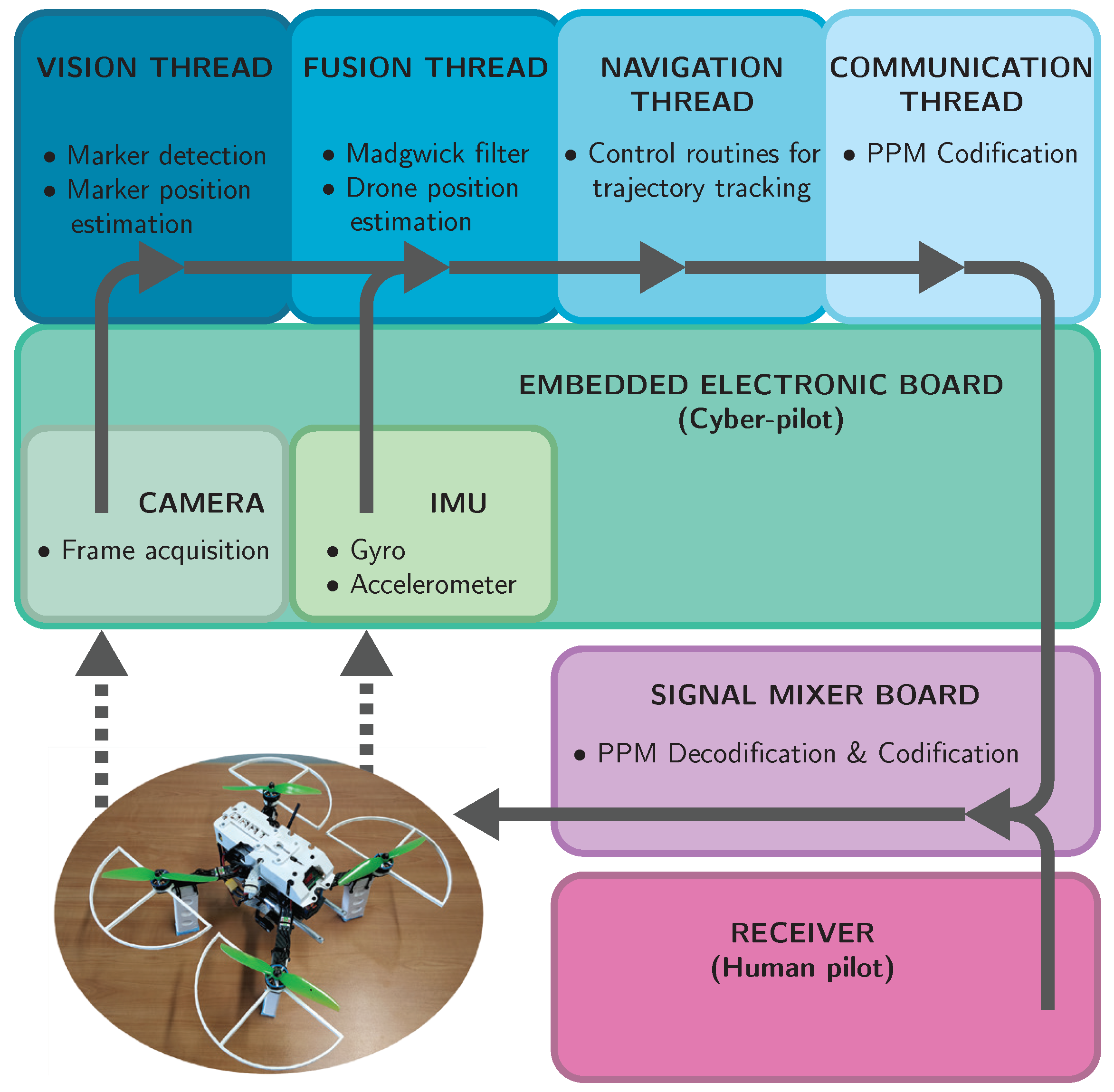
4. Tasks Architecture and Managing
5. Experimental Tests
5.1. Validation of the On-Board Computer Vision System
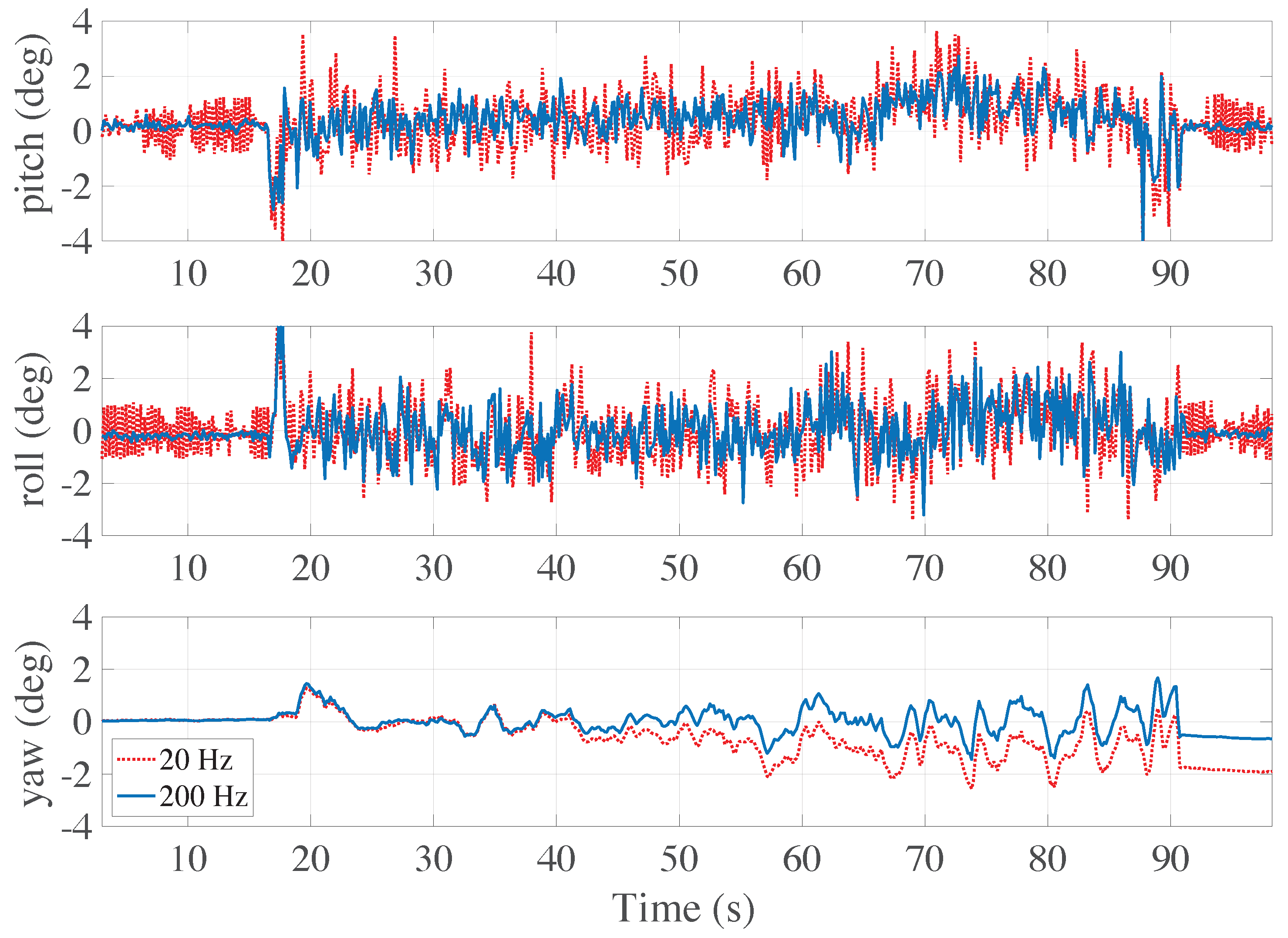
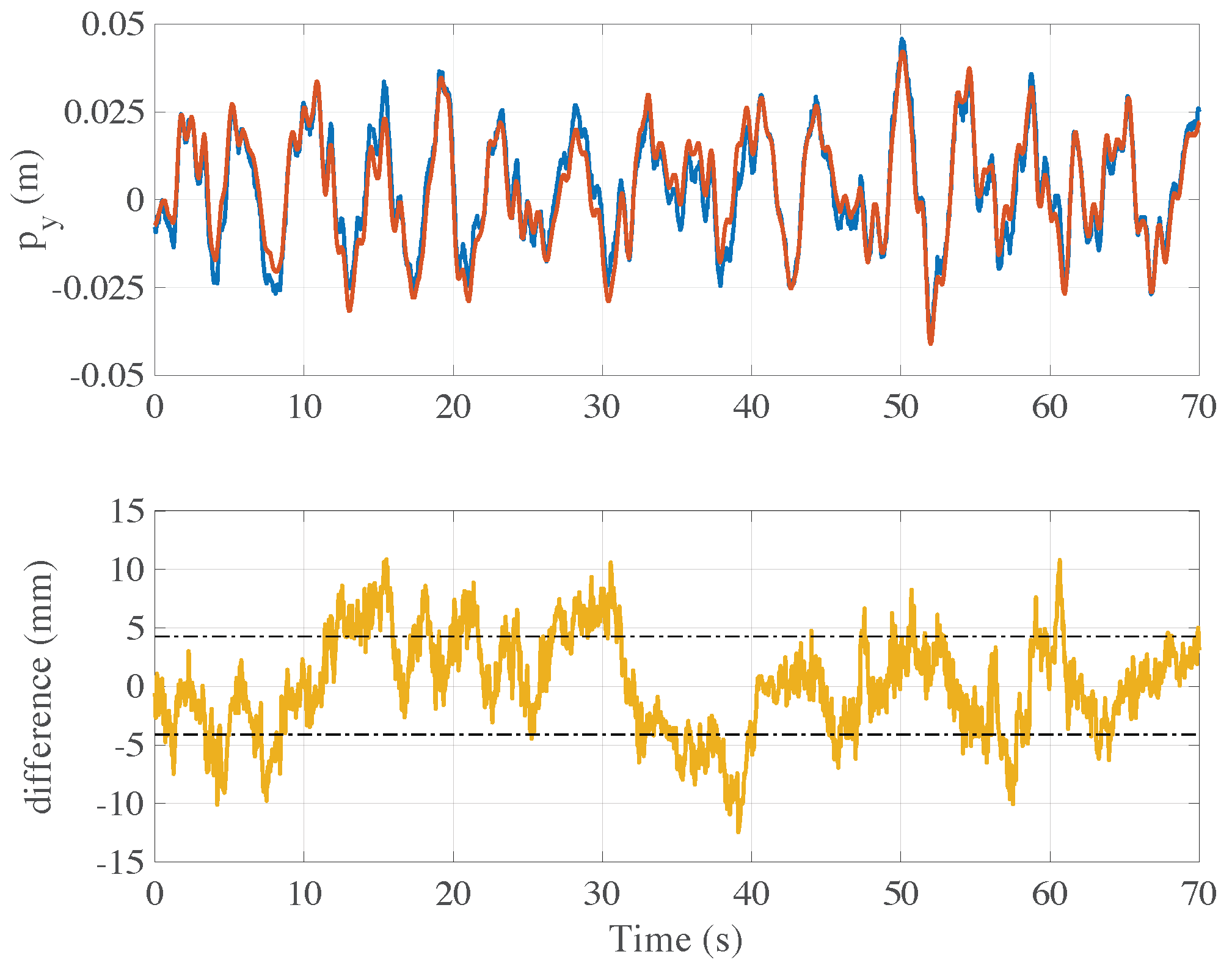
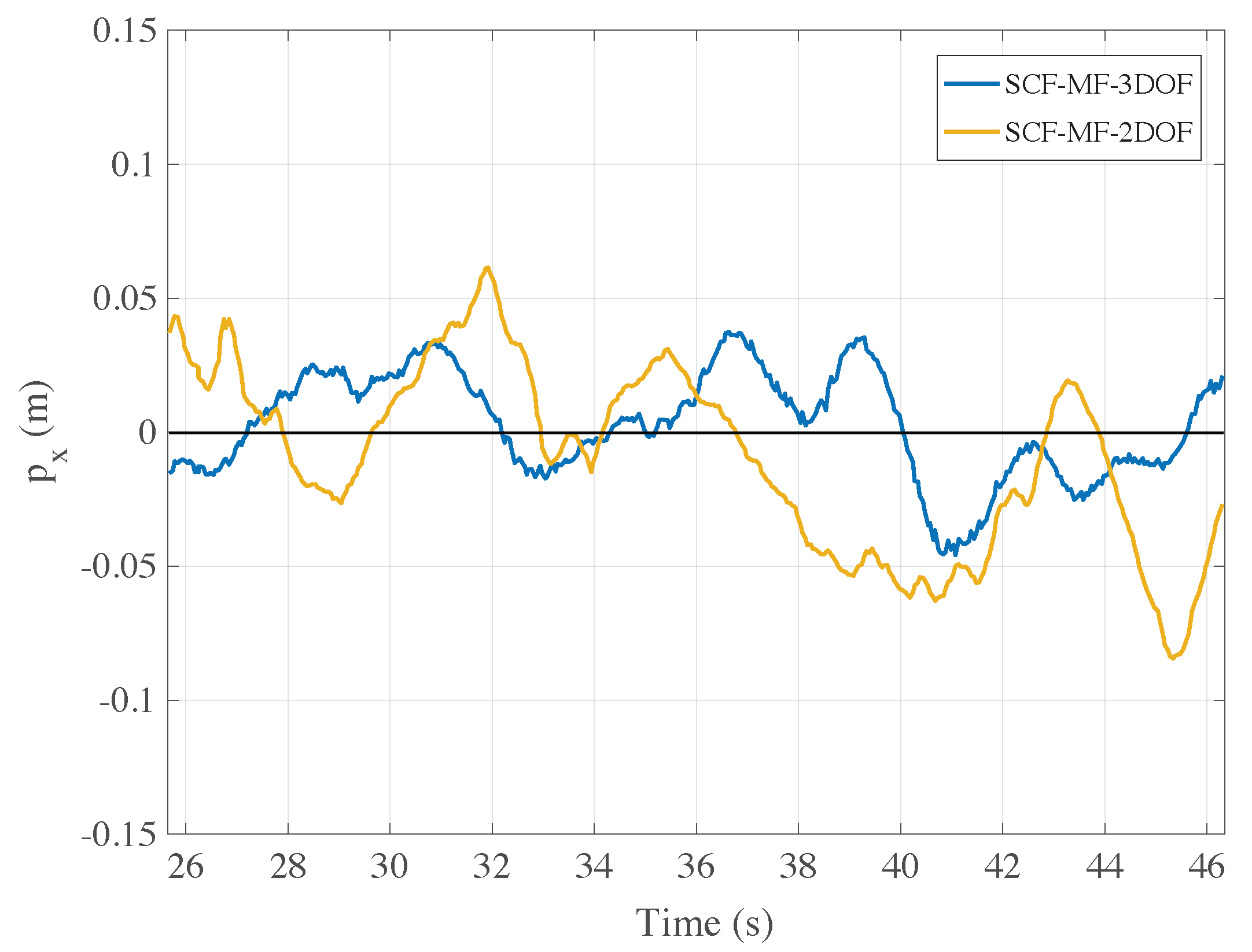
5.2. Comparison between the Position Estimation Methods
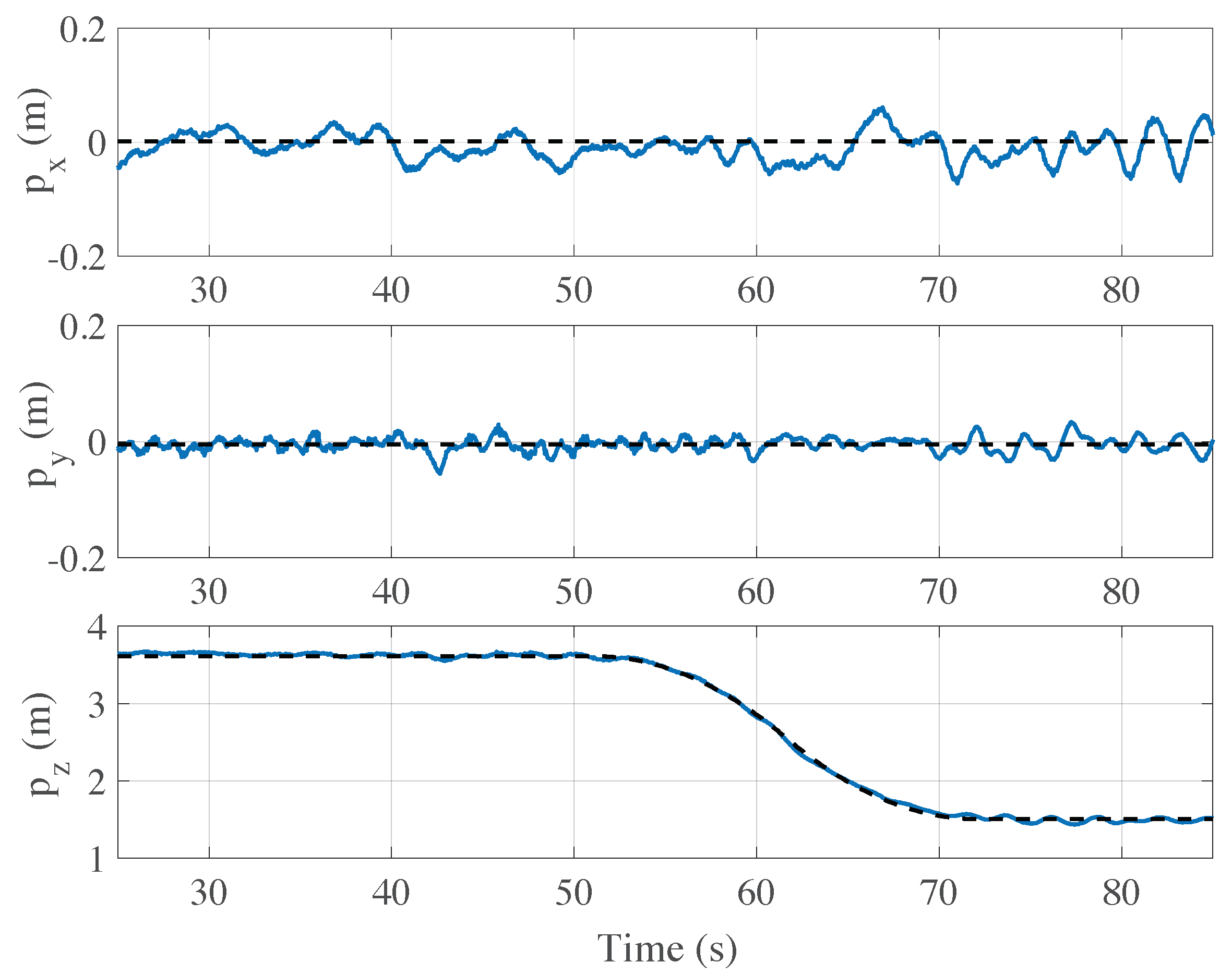
5.3. Autonomous Flight Test
6. Conclusions
Author Contributions
Funding
Institutional Review Board Statement
Informed Consent Statement
Data Availability Statement
Acknowledgments
Conflicts of Interest
Abbreviations
| DOF | Degrees of freedom |
| IMU | Inertial measurement unit |
| UAV | Unmanned aerial vehicle |
| PID | Proportional–integral–derivative |
| PPM | Pulse position modulation |
| NED | North-east-down |
| FIFO | First input first output |
| FPS | Frame per second |
| FCF-CF | Fixed camera frame complementary filter |
| FCF-MF | Fixed camera frame Madgwick filter |
| SCF-MF-2DOF | Stabilized camera frame Madgwick filter 2DOF |
| SCF-MF-3DOF | Stabilized camera frame Madgwick filter 3DOF |
References
- Chan, K.W.; Nirmal, U.; Cheaw, W.G. Progress on drone technology and their applications: A comprehensive review. AIP Conf. Proc. 2018, 2030, 020308. [Google Scholar]
- Shakhatreh, H.; Sawalmeh, A.H.; Al-Fuqaha, A.; Dou, Z.; Almaita, E.; Khalil, I.; Othman, N.S.; Khreishah, A.; Guizani, M. Unmanned aerial vehicles (UAVs): A survey on civil applications and key research challenge. IEEE Access 2019, 7, 48572–48634. [Google Scholar] [CrossRef]
- Shakeri, R.; Al-Garadi, M.A.; Badawy, A.; Mohamed, A.; Khattab, T.; Al-Ali, A.K.; Harras, K.A.; Guizani, M. Design challenges of multi-UAV systems in cyber-physical applications: A comprehensive survey and future directions. IEEE Commun. Surv. Tutor. 2019, 21, 3340–3385. [Google Scholar] [CrossRef] [Green Version]
- Wang, X.; Huang, Z.; Sui, G.; Lian, H. Analysis on the development trend of future UAV equipment technology. Acad. J. Eng. Technol. Sci. 2019, 2. [Google Scholar] [CrossRef]
- Ghazzai, H.; Menouar, H.; Kadri, A.; Massoud, Y. Future UAV-based ITS: A comprehensive scheduling framework. IEEE Access 2019, 7, 75678–75695. [Google Scholar] [CrossRef]
- Alsalam, B.H.Y.; Morton, K.; Campbell, D.; Gonzalez, F. Autonomous UAV with vision based on-board decision making for remote sensing and precision agriculture. In Proceedings of the 2017 IEEE Aerospace Conference, Big Sky, MT, USA, 4–11 March 2017. [Google Scholar]
- Tokekar, P.; Hook, J.V.; Mulla, D.; Isler, V. Sensor planning for a symbiotic UAV and UGV system for precision agriculture. IEEE Trans. Robot. 2016, 32, 1498–1511. [Google Scholar] [CrossRef]
- Kim, J.; Kim, S.; Ju, C.; Son, H.I. Unmanned aerial vehicles in agriculture: A review of perspective of platform, control, and applications. IEEE Access 2019, 7, 105100–105115. [Google Scholar] [CrossRef]
- Henkel, P.; Mittmann, U.; Iafrancesco, M. Real-time kinematic positioning with GPS and GLONASS. In Proceedings of the 2016 24th European Signal Processing Conference (EUSIPCO), Budapest, Hungary, 29 August–2 September 2016; pp. 1063–1067. [Google Scholar]
- Jordan, S.; Moore, J.; Hovet, S.; Box, J.; Perry, J.; Kirsche, K.; Lewis, D.; Tse, Z.T.H. State-of-the-art technologies for UAV inspections. IET Radar Sonar Navig. 2018, 12, 151–164. [Google Scholar] [CrossRef]
- Dinesh, M.A.; Kumar, S.S.; Sanath, J.; Akarsh, K.N.; Gowda, K.M.M. Development of an Autonomous Drone for Surveillance Application. Proc. Int. Res. J. Eng. Technol. IRJET 2018, 5, 331–333. [Google Scholar]
- Saska, M. Large sensors with adaptive shape realised by self-stabilised compact groups of micro aerial vehicles. Robot. Res. 2020, 10, 101–107. [Google Scholar]
- Lu, L.; Redondo, C.; Campoy, P. Optimal Frontier-Based Autonomous Exploration in Unconstructed Environment Using RGB-D Sensor. Sensors 2020, 20, 6507. [Google Scholar] [CrossRef] [PubMed]
- Zhou, H.; Kong, H.; Wei, L.; Creighton, D.; Nahavandi, S. Efficient road detection and tracking for unmanned aerial vehicle. IEEE Trans. Intell. Transp. Syst. 2015, 16, 297–309. [Google Scholar] [CrossRef]
- Srini, V.P. A vision for supporting autonomous navigation in urban environments. Computer 2006, 39, 68–77. [Google Scholar] [CrossRef]
- Nonami, K. Research and Development of Drone and Roadmap to Evolution. J. Robot. Mechatron. 2018, 30, 322–336. [Google Scholar] [CrossRef]
- Elloumi, M.; Dhaou, R.; Escrig, B.; Idoudi, H.; Saidane, L.A. Monitoring road traffic with a UAV-based system. In Proceedings of the 2018 IEEE Wireless Communications and Networking Conference (WCNC), Barcelona, Spain, 15–18 April 2018; pp. 1–6. [Google Scholar]
- Cheng, L.; Zhong, L.; Tian, S.; Xing, J. Task Assignment Algorithm for Road Patrol by Multiple UAVs With Multiple Bases and Rechargeable Endurance. IEEE Access 2019, 7, 144381–144397. [Google Scholar] [CrossRef]
- Erdelj, M.; Król, M.; Natalizio, E. Wireless sensor networks and multi-UAV systems for natural disaster management. Comput. Netw. 2017, 124, 72–86. [Google Scholar] [CrossRef]
- Ren, H.; Zhao, Y.; Xiao, W.; Hu, Z. A review of UAV monitoring in mining areas: Current status and future perspectives. Int. J. Coal Sci. Technol. 2019, 6, 320–333. [Google Scholar] [CrossRef] [Green Version]
- Erdelj, M.; Natalizio, E.; Chowdhury, K.R.; Kaushik, R.; Akyildiz, I.F. Help from the sky: Leveraging UAVs for disaster management. IEEE Pervasive Comput. 2017, 16, 24–32. [Google Scholar] [CrossRef]
- Avanzato, R.; Beritelli, F. A Smart UAV-Femtocell Data Sensing System for Post-Earthquake Localization of People. IEEE Access 2020, 8, 30262–30270. [Google Scholar] [CrossRef]
- Aljehani, M.; Inoue, M. Performance evaluation of multi-UAV system in post-disaster application: Validated by HITL simulator. IEEE Access 2019, 7, 64386–64400. [Google Scholar] [CrossRef]
- Alotaibi, E.T.; Alqefari, S.S.; Koubaa, A. Lsar: Multi-uav collaboration for search and rescue missions. IEEE Access 2019, 7, 55817–55832. [Google Scholar] [CrossRef]
- Petrlík, M.; Báča, T.; Heřt, D.; Vrba, M.; Krajník, T.; Saska, M. A Robust UAV System for Operations in a Constrained Environment. IEEE Robot. Autom. Lett. 2020, 5, 2169–2176. [Google Scholar] [CrossRef]
- Zhang, J.; Wu, Y.; Liu, W.; Chen, X. Novel Approach to Position and Orientation Estimation in Vision-Based UAV Navigation. IEEE Trans. Aerosp. Electron. Syst. 2010, 46, 687–700. [Google Scholar] [CrossRef]
- Cesetti, A.; Frontoni, E.; Mancini, A.; Zingaretti, P.; Longhi, S. A Vision-Based Guidance System for UAV Navigation and Safe Landing using Natural Landmarks. J. Intell. Robot. Syst. 2010, 57, 233. [Google Scholar] [CrossRef]
- Khansari-Zadeh, S.M.; Saghafi, F. Vision-Based Navigation in Autonomous Close Proximity Operations using Neural Networks. IEEE Trans. Aerosp. Electron. Syst. 2011, 47, 864–883. [Google Scholar] [CrossRef]
- Zhang, J.; Liu, W.; Wu, Y. Novel Technique for Vision-Based UAV Navigation. IEEE Trans. Aerosp. Electron. Syst. 2011, 47, 2731–2741. [Google Scholar] [CrossRef]
- Carrillo, L.R.G.; Lopez, A.E.D.; Lozano, R.; Pegard, C. Combining Stereo Vision and Inertial Navigation System for a Quad-Rotor UAV. J. Intell. Robot. Syst. 2012, 65, 373–387. [Google Scholar] [CrossRef]
- Aguilar, W.G.; Salcedo, V.S.; Sandoval, D.S.; Cobena, B. Developing of a Video-Based Model for UAV Autonomous Navigation. In 2017 Latin American Workshop on Computational Neuroscience (LAWCN): Computational Neuroscience; Springer: Cham, Switzerland, 2017; pp. 94–105. [Google Scholar]
- Miller, B.M.; Stepanyan, K.V.; Popov, A.K.; Miller, A.B. UAV navigation based on videosequences captured by the onboard video camera. Autom. Remote Control 2017, 78, 2211–2221. [Google Scholar] [CrossRef]
- Lu, Y.; Xue, Z.; Xia, G.-S.; Zhang, L. A survey on vision-based UAV navigation. Geo-Spat. Inf. Sci. 2018, 21, 21–32. [Google Scholar] [CrossRef] [Green Version]
- Rodriguez-Ramos, A.; Alvarez-Fernandez, A.; Bavle, H.; Campoy, P.; How, J.P. Vision-Based Multirotor Following Using Synthetic Learning Techniques. Sensors 2019, 19, 4794. [Google Scholar] [CrossRef] [Green Version]
- Mademlis, I.; Torres-González, A.; Capitán, J.; Cunha, R.; Guerreiro, B.J.N.; Messina, A.; Negro, F.; Barz, C.L.; Gonçalves, T.F.; Tefas, A.; et al. A multiple-uav software architecture for autonomous media production. In Proceedings of the Workshop on Signal Processing Computer vision and Deep Learning for Autonomous Systems (EUSIPCO2019), A Coruna, Spain, 2–6 September 2019. [Google Scholar]
- Mademlis, I.; Nikolaidis, N.; Tefas, A.; Pitas, I.; Wagner, T.; Messina, A. Autonomous UAV cinematography: A tutorial and a formalized shot-type taxonomy. ACM Comput. Surv. CSUR 2019, 52, 1–33. [Google Scholar] [CrossRef]
- GPS Accuracy, Official U.S. Government Information about the Global Positioning System (GPS) and Related Topics. Available online: https://www.gps.gov/systems/gps/performance/accuracy/ (accessed on 12 December 2020).
- Zhao, S.; Chen, Y.; Farrell, J.A. High-precision vehicle navigation in urban environments using an MEM’s IMU and single-frequency GPS receiver. IEEE Trans. Intell. Transp. Syst. 2016, 17, 2854–2867. [Google Scholar] [CrossRef]
- Lu, Q.; Zhang, Y.; Lin, J.; Wu, M. Dynamic Electromagnetic Positioning System for Accurate Close-Range Navigation of Multirotor UAVs. IEEE Sens. J. 2020, 20, 4459–4468. [Google Scholar] [CrossRef]
- Liu, H.; Yang, B. Quadrotor Singularity Free Modeling and Acrobatic Maneuvering. In Proceedings of the International Design Engineering Technical Conferences and Computers and Information in Engineering Conference, Anaheim, CA, USA, 18–21 August 2019; Volume 59230, p. V05AT07A055. [Google Scholar]
- Yang, Q.; Zhang, J.; Shi, G.; Hu, J.; Wu, Y. Maneuver decision of UAV in short-range air combat based on deep reinforcement learning. IEEE Access 2019, 8, 363–378. [Google Scholar] [CrossRef]
- Padhy, R.P.; Xia, F.; Choudhury, S.K.; Sa, P.K.; Bakshi, S. Monocular Vision Aided Autonomous UAV Navigation in Indoor Corridor Environments. IEEE Trans. Sustain. Comput. 2019, 4, 96–108. [Google Scholar] [CrossRef]
- Grzonka, S.; Grisetti, G.; Burgard, W. A Fully Autonomous Indoor Quadrotor. IEEE Trans. Robot. 2012, 28, 90–100. [Google Scholar] [CrossRef] [Green Version]
- How, J.P.; Behihke, B.; Frank, A.; Dale, D.; Vian, J. Real-time indoor autonomous vehicle test environment. IEEE Control Syst. Mag. 2008, 28, 51–64. [Google Scholar] [CrossRef]
- Yang, S.; Scherer, S.A.; Yi, X.; Zell, A. Multi-camera visual SLAM for autonomous navigation of micro aerial vehicles. Robot. Auton. Syst. 2017, 93, 116–134. [Google Scholar] [CrossRef]
- Mac, T.T.; Copot, C.; Keyser, R.D.; Ionescu, C.M. The development of an autonomous navigation system with optimal control of an UAV in partly unknown indoor environment. Mechatronics 2018, 49, 187–196. [Google Scholar] [CrossRef]
- Mustafah, Y.M.; Azman, A.W.; Akbar, F. Indoor UAV Positioning Using Stereo Vision Sensor. Procedia Eng. 2012, 41, 575–579. [Google Scholar] [CrossRef] [Green Version]
- Zhang, J.; Wang, X.; Yu, Z.; Lyu, Y.; Mao, S.; Periaswamy, S.C.G.; Patton, J.; Wang, X. Robust rfid based 6-dof localization for unmanned aerial vehicles. IEEE Access 2019, 7, 77348–77361. [Google Scholar] [CrossRef]
- Balderas, L.I.; Reyna, A.; Panduro, M.A.; Rio, C.D.; Gutiérrez, A.R. Low-profile conformal UWB antenna for UAV applications. IEEE Access 2019, 7, 127486–127494. [Google Scholar] [CrossRef]
- You, W.; Li, F.; Liao, L.; Huang, M. Data Fusion of UWB and IMU Based on Unscented Kalman Filter for Indoor Localization of Quadrotor UAV. IEEE Access 2020, 8, 64971–64981. [Google Scholar] [CrossRef]
- Gonzalez-Sieira, A.; Cores, D.; Mucientes, M.; Bugarin, A. Autonomous navigation for UAVs managing motion and sensing uncertainty. Robot. Auton. Syst. 2020, 126, 103455. [Google Scholar] [CrossRef]
- Imanberdiyev, N.; Fu, C.; Kayacan, E.; Chen, I.-M. Autonomous navigation of UAV by using real-time model-based reinforcement learning. In Proceedings of the 2016 14th International Conference on Control, Automation, Robotics and Vision (ICARCV), Phuket, Thailand, 13–15 November 2016; pp. 1–6. [Google Scholar]
- Lugo, J.J.; Zell, A. Framework for Autonomous On-board Navigation with the AR. Drone. J. Intell. Robot. Syst. 2014, 73, 401–412. [Google Scholar] [CrossRef]
- Basso, M.; Bigazzi, L.; Innocenti, G. DART Project: A High Precision UAV Prototype Exploiting On-board Visual Sensing. In Proceedings of the 15th International Conference on Autonomic and Autonomous Systems (ICAS), Athens, Greece, 2–6 June 2019. [Google Scholar]
- Kim, J.-H.; Sukkarieh, S.; Wishart, S. Real-Time Navigation, Guidance, and Control of a UAV Using Low-Cost Sensors. Field Serv. Robot. 2006, 24, 299–309. [Google Scholar]
- Gageik, N.; Benz, P.; Montenegro, S. Obstacle detection and collision avoidance for a UAV with complementary low-cost sensors. IEEE Access 2015, 3, 599–609. [Google Scholar] [CrossRef]
- RIIS Blog, Four Drone Manufacturers Providing SDKs. Available online: https://riis.com/blog/four_drone_sdks/ (accessed on 12 December 2020).
- Wang, J.; Olson, E. AprilTag2: Efficient and robust fiducial detection. In Proceedings of the 2016 IEEE/RSJ International Conference on Intelligent Robots and Systems (IROS), Daejeon, Korea, 9–14 October 2016. [Google Scholar]
- Madgwick, S.O.H. An efficient orientation filter for inertial and inertial/magnetic sensor arrays. Rep. x-io Univ. Bristol UK 2010, 25, 113–118. [Google Scholar]
- Gebre-Egziabher, D.; Hayward, R.C.; Powell, J.D. Design of multi-sensor attitude determination systems. IEEE Trans. Aerosp. Electron. Syst. 2004, 40, 627–649. [Google Scholar] [CrossRef]
- Sabatini, A.M. Quaternion-based extended Kalman filter for determining orientation by inertial and magnetic sensing. IEEE Trans Biomed. Eng. 2006, 53, 1346–1356. [Google Scholar] [CrossRef]


| Algorithm | Standard Deviation (Along y) |
|---|---|
| FCF-CF | 5.35 cm |
| FCF-MF | 4.01 cm |
| SCF-2DOF | 1.77 cm |
| Algorithm | Standard Deviation (Along x) |
|---|---|
| SCF-2DOF | 3.42 cm |
| SCF-3DOF | 2.54 cm |
Publisher’s Note: MDPI stays neutral with regard to jurisdictional claims in published maps and institutional affiliations. |
© 2021 by the authors. Licensee MDPI, Basel, Switzerland. This article is an open access article distributed under the terms and conditions of the Creative Commons Attribution (CC BY) license (http://creativecommons.org/licenses/by/4.0/).
Share and Cite
Bigazzi, L.; Gherardini, S.; Innocenti, G.; Basso, M. Development of Non Expensive Technologies for Precise Maneuvering of Completely Autonomous Unmanned Aerial Vehicles. Sensors 2021, 21, 391. https://0-doi-org.brum.beds.ac.uk/10.3390/s21020391
Bigazzi L, Gherardini S, Innocenti G, Basso M. Development of Non Expensive Technologies for Precise Maneuvering of Completely Autonomous Unmanned Aerial Vehicles. Sensors. 2021; 21(2):391. https://0-doi-org.brum.beds.ac.uk/10.3390/s21020391
Chicago/Turabian StyleBigazzi, Luca, Stefano Gherardini, Giacomo Innocenti, and Michele Basso. 2021. "Development of Non Expensive Technologies for Precise Maneuvering of Completely Autonomous Unmanned Aerial Vehicles" Sensors 21, no. 2: 391. https://0-doi-org.brum.beds.ac.uk/10.3390/s21020391