1. Introduction
Commercial unmanned surface vehicle (USV) systems are used in many operations such as harbor inspection, surveillance, mapping, data acquisition, oceanography, etc. (see
Figure 1 and
Figure 2). This creates a need for low-cost sensor systems to operate a USV safely with satisfactory performance. The autopilot system is a critical component that is used for turning and path following. Both heading and course autopilots can be used for this purpose. Course autopilots are the preferred solution during path following. However, for stationkeeping it is necessary to control the heading angle. The reason for this is that the course angle is not defined at zero speed.
Ships are usually equipped with a gyrocompass, which is a nonmagnetic compass able to find true North using a fast-spinning gyroscope (Fossen [
1]). The gyrocompass gives a highly accurate measurement of the heading (yaw) angle, but it is too expensive to be used in small USV systems. Hence, it is tempting to use a low-cost magnetic compass for navigation and maneuvering. This is not straightforward since a magnetic compass is susceptible to magnetic disturbances produced by electromagnetic devices such as propellers and thrusters. In addition, the magnetic field of the Earth is not perfectly aligned but skewed along the Earth’s rotational axis. The skew or bias is called declination, and it must be compensated for when navigating.
An alternative measurement to the compass could be to use two GNSS antennas on the same receiver with a known offset vector to compute the heading angle. The accuracy is further improved by using real-time kinematic (RTK) GNSS positioning (Farrell [
2]). This is the preferred solution for small USVs since the offset vector can be small. It is well known that the RTK GNSS receivers are sensitive to ionospheric disturbances, multipath, loss of signals, the number of available satellites, etc., so the reliability can, in many cases, be unsatisfactory.
The scope of this article is to derive a robust state estimator for SOG, COG, and course rate such that these signals can be used to design a USV course autopilot for path following. The state estimator should only use the North–East positions, alternatively the latitude and longitude, of a GNSS receiver. If the course angle is available as a direct measurement or an estimate, it is straightforward to design a proportional-integral-derivative (PID) controller for course control; see Fossen [
1].
The dynamics of a USV moving along a path or a trajectory can be modeled by using 2D target-tracking models (Li and Jilkov [
4]). The simplest models for a target-tracking maneuver are the white-noise constant velocity (CV) and constant acceleration (CA) models (Bar-Shalom et al. [
5]). These models are based on the assumption that the target speed or acceleration are independent processes driven by Gaussian white noise. The Otter and Mariner USVs shown in
Figure 1 and
Figure 2, respectively, are not able to produce aggressive linear accelerations. Hence, the CV model is well suited to describe the vehicle’s speed
U during path-following control, since
U is nearly constant even though the USV experiences small linear accelerations. Analysis of automatic identification system (AIS) data confirms this (Siegert et al. [
6]). However, both USVs have propellers that can turn the vehicles quite fast. This suggests that the course angle
should be modeled by a CA model. Consequently, the target-tracking models are chosen as a combination of the CV and CA models according to
where
and
are Gaussian white-noise processes. The models (
1)–(3) will be used as a basis for the EKF presented in
Section 3.
The main result of this article is a five-state EKF (
Appendix A) aided by GNSS positions or latitude–longitude measurements, which is intended for course and path-following control. The EKF can also be used to process AIS measurements (Fossen and Fossen [
7]) with the purpose of ship motion prediction. The algorithm is computationally efficient and easy to implement. The main advantage of the EKF is that vendors do not need to use COG and SOG measurements from GNSS receivers, which have varying quality. In addition, the algorithm produces an accurate estimate of the course rate, which is an important signal when implementing PID course autopilot systems.
The remainder of this article is organized as follows:
Section 2 presents the kinematic equations of a surface vehicle, while
Section 3 contains the EKF for COG, SOG, and course rate estimation.
Section 4 describes a method for USV course autopilot design.
Section 5 includes a simulation study of a small USV under course autopilot control, while
Section 6 and
Section 7 present the experimental results using two commercial USV systems. The discussion and concluding remarks are drawn in
Section 8 and
Section 9.
2. Kinematics
The relationship between the angular variables
course, heading, and
crab angle is important for maneuvering of a USV in the horizontal plane. The terms course and heading are used interchangeably in much of the literature on marine systems, and this leads to confusion. Let the BODY and North-East-Down (NED) reference frames in
Figure 3 be denoted by
and
, respectively.
Definition 1. (Yaw or heading angle ) The angle ψ from the axis (true North) to the axis of the USV, positive rotation about the axis by the right-hand screw convention.
The heading angle is usually measured by using a magnetic compass, gyrocompass or two GNSS receivers; see Gade [
8] for a discussion of methods. The heading angle is well defined for zero speed such that it is possible to design a
heading autopilot to maintain constant heading during stationkeeping and transit. However, during transit it is common to use a
course autopilot for path following.
Definition 2. (Course angle ) The angle χ from the axis (true North) to the velocity vector of the USV, positive rotation about the axis by the right-hand screw convention.
Note that the course angle is only defined for positive speed. The North–East positions
of a USV can be described by (Fossen [
1]),
where
are the surge and sway velocities, respectively. These equations can be expressed in
amplitude-phase form by
where the course angle is defined as
Furthermore, the amplitude
U and phase variable
are
Note that U is the speed in the horizontal plane, and is the crab angle.
Definition 3. (Crab angle ) The angle from the axis to the velocity vector of the USV, positive rotation about the axis by the right-hand screw convention.
3. EKF for SOG, COG and Course Rate
The primary objective of the EKF is to compute accurate estimates of the SOG, COG, and course rate of the USV when moving along a path. The dynamic model of the EKF ensures that old GNSS position measurements are used to compute the estimates. Since the path is not parametrized and the heading angle is unknown, the only information during path following is the measured GNSS position, alternatively the latitude-longitude pair.
3.1. Five-State EKF: North-East Position Measurements
The North–East positions
of the USV are given by (
6) and (7), while the speed and the course angle are modeled by the CV and CA models (
1)–(3). The resulting state–space model expressed in North–East coordinates is
where
and
are Gaussian white-noise process noise. Two small constants
and
have been added to the model to ensure that
U and
converge to zero during stationkeeping. Equations (13) and (14) are referred to as
Singer models [
9] in the target-tracking community (Li and Jilkov [
4]).
The GNSS measurement equations associated with (
11)–(14) are
where
and
are Gaussian white-noise measurement noise. For the speed Equation (13), simulation studies revealed that the CV model with the Singer modification
was most accurate for USVs since the speed is
nearly-constant most of the time, i.e., small linear accelerations. Turning was accurately described by using the CA model with
. This gave satisfactory course rate estimates.
The discrete-time representation of (
11)–(14) is obtained by Euler’s method
where
h is used to denote the sampling time. The discrete-time measurement equations are
Consequently, the discrete-time state–space model becomes
where
The resulting EKF algorithm (see Brown and Hwang [
10]) is summarized in
Table 1 where
, and
and
are the covariance matrices for the process and measurement noises. The
a priori state and covariance matrix estimates (before update) are denoted
, while the
a posteriori state and covariance matrix estimates (after update) are denoted by
.
3.2. Five-State EKF: Latitude and Longitude Measurements
GNSS receivers output latitude,
, longitude,
l, and elevation,
h, using the World Geodetic System (WGS-84) ellipsoid as reference system [
11]. For vehicles operating on the sea surface, we chose the height above the reference geoid as
. The coordinate origin is conveniently fixed at a point on Earth’s surface, specified by its latitude and longitude pair
. The Earth radius of curvature in the prime vertical,
, and the radius of curvature in the meridian,
, are (Farrell [
2]),
where
is the semi-minor axis (equatorial radius), and
is the Earth eccentricity (WGS-84). Consequently, the latitude and longitude dynamics are
where
and
are the North–East velocities of the vehicle. The discrete-time EKF model for longitude and latitude are obtained by Euler’s method
The state–space representation is
where
The Jacobians are
where
and
4. USV Course Autopilot Design
The course angle dynamics can be approximated by a first-order model (Nomoto [
12])
where
T is the time constant in yaw, and
K is implicitly defined by the ratio
Here, is the moment of inertia, is the hydrodynamic added moment of inertia, is the yaw moment, and is a time-varying disturbance due to unmodeled dynamics and environmental disturbances. In practice, will be a nearly constant drift term, which can be compensated by an integral controller.
The Nomoto gain and time constants
K and
T, respectively, can be determined by a maneuvering test. e.g., a turning circle or a zigzag test (Fossen [
1]). The course autopilot was chosen as a PID controller with reference feedforward
where
is the commanded yaw moment,
is the proportional gain,
is the derivative time constant, and
is the integral time constant. The course angular velocity tracking error is denoted by
, where the subscript
d denotes the desired value. The unconstrained course angle tracking error
is mapped to the interval
using the operator
representing the smallest-signed angle (SSA) or difference between the two angles
and
. The Marine Systems Simulator (MSS) Matlab implementation is (Fossen and Perez [
13]),
![Sensors 21 07910 i001]()
The reference feedforward signal was chosen as
where
and
are the desired angular velocity and acceleration, respectively. The resulting closed-loop system is
The PID controller gains can be determined by pole placement with
and
as design parameters. This gives
The integrator time constant was chosen such that
. In other words,
This guarantees that the tracking errors
and
converge exponentially to zero under the assumption that
. Global exponential stability cannot be proven since the course angle error is defined on
and not
as shown by Bhat and Bernstein [
14].
5. Simulation Study of the Otter USV
In the simulation study, a mathematical model of the Maritime Robotics Otter USV, length
, was used. The model is included in the Matlab MSS toolbox (Fossen and Perez [
13]) as a function
which returns the time derivative, xdot, of the state vector
The inputs are the left and right propeller shaft speeds n = [n1,n2]’, the mass of the payload, m_p, the location of the payload, r_p = [x_p,y_p,z_p]’, ocean current speed, V_c, and ocean current direction, beta_c. The toolbox also has a Simulink block for numerical integration of the m-file function.
Estimation of SOG, COG and Course Rate during Course Autopilot Control
In the simulation study, the five-state EKF in
Section 3.1 was used to estimate the course angle and course rate, which are the feedback signals needed to implement the course autopilot (
46). The filter sampling frequency was chosen as
, while the GNSS position measurements were received at
.
The MSS Otter USV model is controlled by two propellers with shaft speeds
and
in
. The propellers produce a surge force
and a yaw moment
according to
where
,
and
is the propeller gain.
The operator specifies the desired force
in the surge direction, while the course autopilot (
46) computes the desired yaw moment
. The control allocation problem is solved by applying the inverse mapping
The Nomoto time and gain constants of the Otter USV were estimated to
The course autopilot system was implemented as
where the controller gains are determined by (
49)–(
51) by specifying
and
. This yields
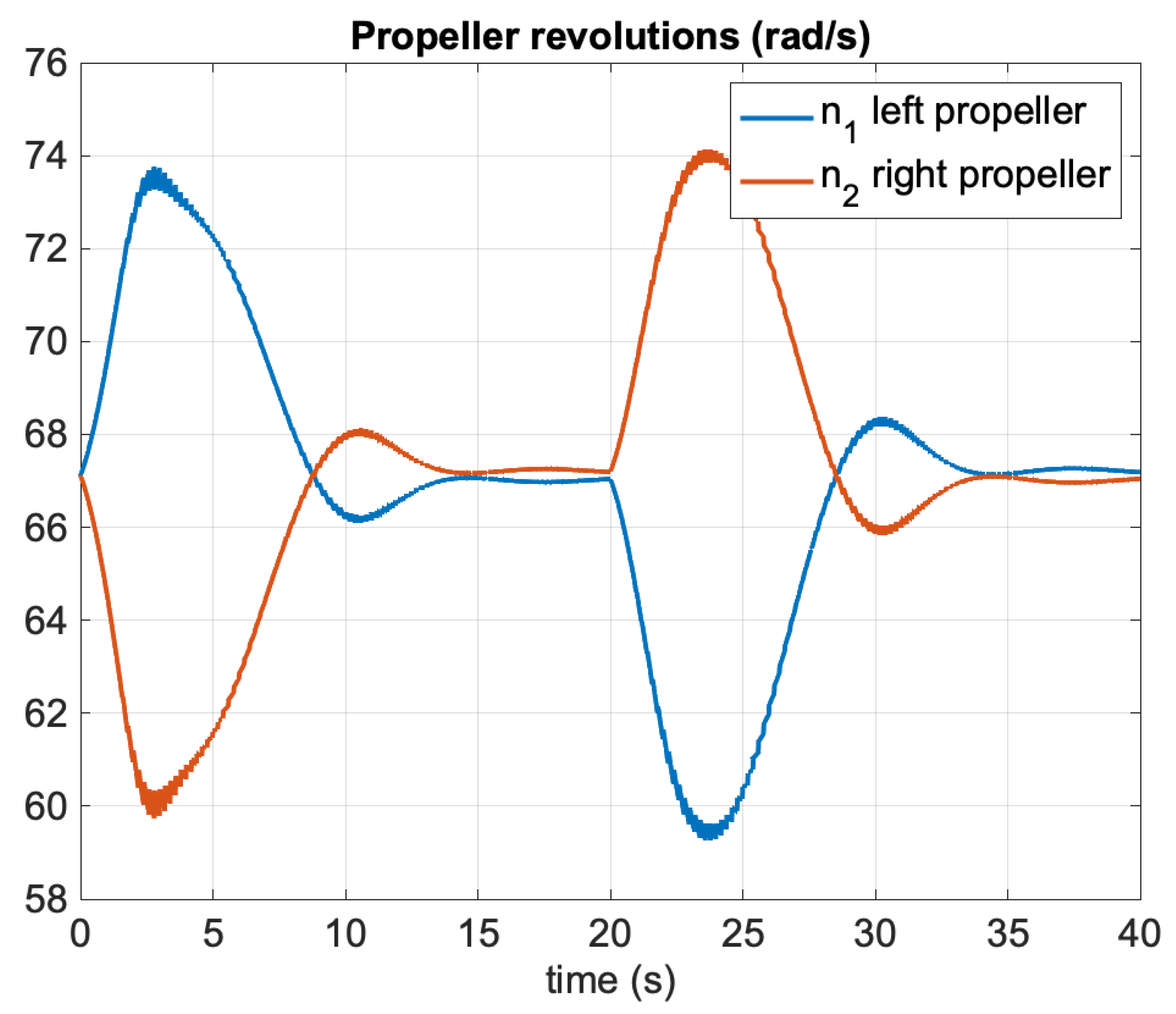
Figure 4 shows the North–East positions during autopilot control. The propeller commands are shown in
Figure 5 where the control allocation algorithm (
53)–(55) was applied.
Figure 6 clearly demonstrates that the EKF was able to estimate the unmeasured states
U,
, and
quite accurately. The zoomed windows show the 5 Hz slow update rate of the filter (GNSS measurements frequency) compared to the 50 Hz sampling frequency of the predictor.
6. Experiments with the Mariner USV
In the first experiment, the Mariner USV was used. The geographical location is shown in
Figure 7. The blue line indicates the traveled path in the Trondheim fjord, Norway. The experiments were performed in sea state 2 corresponding to wave amplitudes below 0.5 m. Latitude and longitude were measured using a u-blox NEO-M8Q GNSS receiver at 5 Hz [
15], while the SOG and COG measurements were complementary measurements used to benchmark the EKF. The accuracy of the NEO-MQ8 in the horizontal plane was 2.5 m when using GPS/Glonass.
It should be noted that the GNSS values for SOG and COG were not validated. Hence, they do not represent groundtruth. Because of this,
Figure 8 only shows the difference between the two algorithms. The GNSS receiver determines the distance between two fixes, and by using the time taken to travel this distance it can deduce its speed. The COG and SOG can therefore seem erratic under certain conditions. For example, when the USV was moving slowly through rough seas, the antenna moved from side to side as well as in the direction of the vehicle. In contrast, the EKF estimates were not affected by this.
The Kalman filter covariance matrices were chosen as
and
.
Figure 8 shows the performance of the five-state EKF. The EKF succeeded in estimating both the SOG and COG with good accuracy.
7. Experiments with the Otter USV
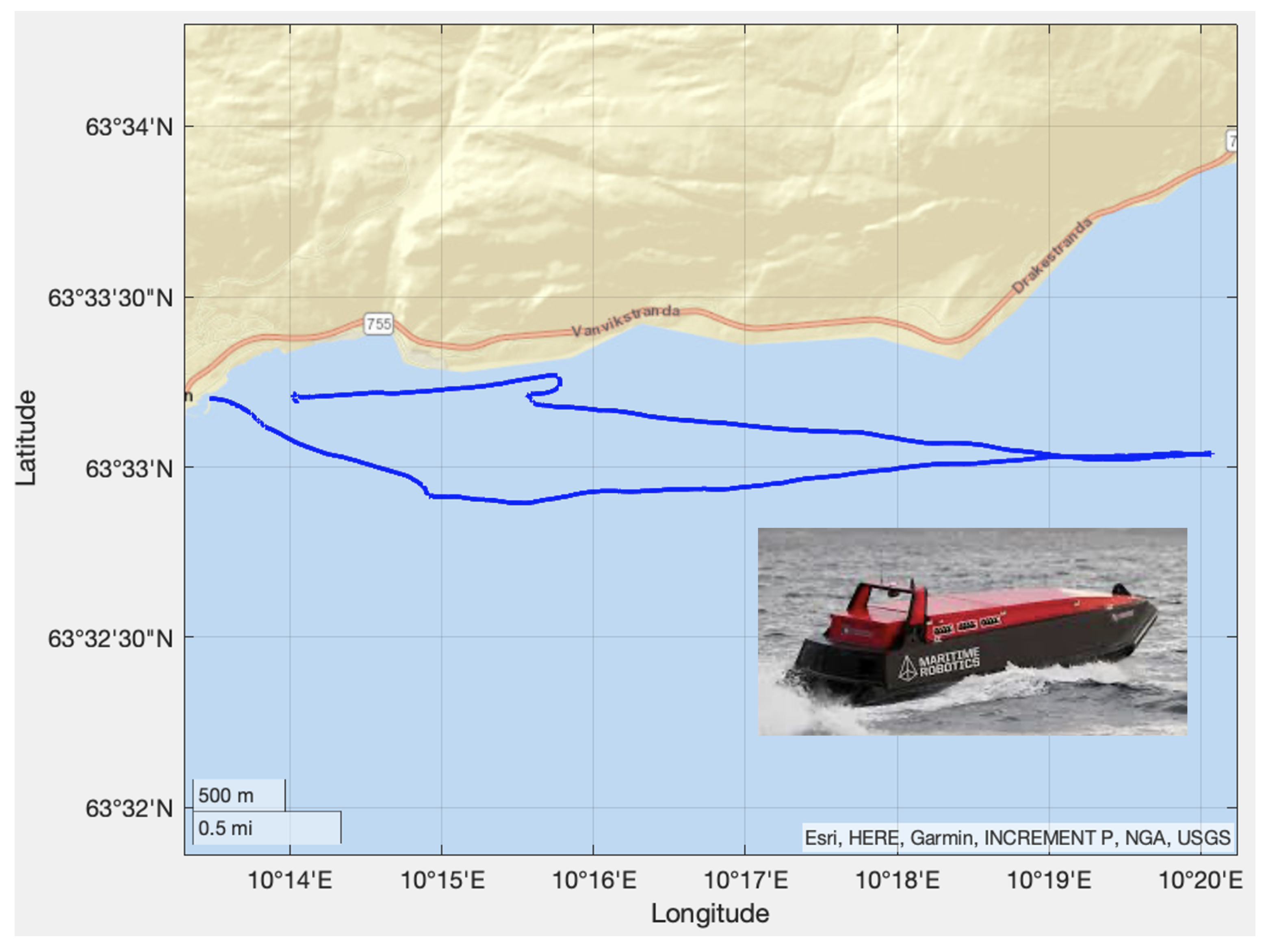
In the second experiment, the Otter USV was used. The USV’s location is shown in
Figure 9. The blue line indicates the traveled path, which is in the proximity of the Maritime Robotics main office in the Trondheim harbor, Norway. The experiments were performed in sea state 1 corresponding to wave amplitudes below 0.1 m. The Otter USV is a much smaller vehicle than the Mariner USV and it typically operates at very low speed (0–2 m/s). This is challenging for the state estimator since the course angle is not defined at zero speed. However, the EKF was stable even at zero speed thanks to the non-zero Singer constants
and
in the model. Latitude and longitude were measured using a u-blox NEO-M8Q GNSS receiver at 5 Hz [
15], while the SOG and COG measurements were complementary measurements used to benchmark the EKF. The filter covariance matrices were chosen as
and
.
The experiment with the Otter USV was repeated, but, the second time, the vehicle was taken out of the harbor to operate in the middle of the Trondheim fjord. However, similar performance was achieved as seen from the plots in
Figure 10 and
Figure 11. From this it can be concluded that the EKF works very well at forward speed while it reaches an arbitrary course angle at zero speed. This is expected since the course angle is not defined at zero speed.
8. Discussion
The experiments with the Otter and Mariner USV systems confirm that the COG, SOG, and course rate can be estimated from latitude and longitude measurements with great accuracy when the speed is above a certain threshold value (typically 0.5 m/s). The experiments also confirm that the speed estimates are less accurate close to zero speed. At zero speed the course angle is not defined. Hence, the course angle estimate will converge to an arbitrary angle in the interval . However, the EKF is exponentially stable at zero speed thanks to the Singer constants in the filter.
9. Conclusions
The main result of the article is a five-state extended Kalman filter (EKF) aided by GNSS latitude-longitude measurements for efficient estimation of course over ground (COG), speed over ground (SOG), and course rate. This is of particular interest for unmanned surface vehicle (USV) systems equipped with low-cost navigation sensor suites. For such systems, a gyrocompass is too expensive compared to the cost of the vehicle. A magnetic compass is unreliable due to electromagnetic interference caused by propellers and thrusters. A dual-antenna GNSS system on the same receiver (RTK GNSS) is an alternative, but the operational reliability (number of dropouts) depends on the density of the reference-station network, number of available satellites, multipath, ionospheric disturbances, etc. Furthermore, it has been demonstrated that the five-state EKF can estimate the SOG, COG, and course rate of a USV quite accurately using a single low-cost u-blox GNSS receiver. It has also been shown that the state estimates can be used to implement course and path-following control systems onboard the USV. The performance of the five-state EKF has been experimentally verified by using navigational data from two commercial USV systems, the Otter and the Mariner USVs by Maritime Robotics, which were operated west of Trondheim, Norway. The results from the experiments demonstrated that the EKF could estimate all states from low-cost latitude–longitude measurements.
Author Contributions
Conceptualization, S.F. and T.I.F.; methodology, S.F. and T.I.F.; software, S.F. and T.I.F.; validation, T.I.F.; investigation, S.F.; data curation, S.F.; writing—original draft preparation, T.I.F. All authors have read and agreed to the published version of the manuscript.
Funding
This work was partially supported by the Research Council (RCN) of Norway through the Center of Excellence funding scheme, SFF AMOS, project number 223254 and the RCN Pilot-T project 296630 RAPP.
Institutional Review Board Statement
Not applicable.
Informed Consent Statement
Not applicable.
Acknowledgments
The authors are grateful to Maritime Robotics AS who contributed USV navigation data and technical expertise. The authors are also grateful for the valuable suggestions and comments by Stephanie Kemna.
Conflicts of Interest
The authors declare no conflict of interest. The funders had no role in the design of the study; in the collection, analyses, or interpretation of data; in the writing of the manuscript, or in the decision to publish the results.
Appendix A. Matlab Function: EKF5states.m
It is straightforward to implement and use the five-state EKF in a practical implementation. The Matlab [
16] function EKF5states.m listed below can be used as template for coding in other languages. The function should be implemented in a loop or a real-time system according to:
![Sensors 21 07910 i002]()
![Sensors 21 07910 i003]()
![Sensors 21 07910 i004]()
References
- Fossen, T.I. Marine Craft Hydrodynamics and Motion Control; John Wiley & Sons.: Chichchester, UK, 2021. [Google Scholar]
- Farrell, J.A. Aided Navigation: GPS with High Rate Sensors; McGraw-Hill: New York, NY, USA, 2008. [Google Scholar]
- Maritime Robotics AS. 2021. Available online: https://www.maritimerobotics.com (accessed on 25 October 2021).
- Li, X.R.; Jilkov, V. Survey of Maneuvering Target Tracking. Part I. Dynamic Models. IEEE Trans. Aerosp. Electron. Syst. 2003, 39, 1333–1364. [Google Scholar] [CrossRef]
- Bar-Shalom, Y.; Li, X.R.; Kirubarajan, T. Estimation with Applications to Tracking and Navigation: Theory, Algorithms and Software; John Wiley & Sons.: New York, NY, USA, 2001. [Google Scholar] [CrossRef]
- Siegert, G.; Banyś, P.; Martinez, C.S.; Heymann, F. EKF Based Trajectory Tracking and Integrity Monitoring of AIS Data. In Proceedings of the 2016 IEEE/ION Position, Location and Navigation Symposium (PLANS), Savannah, GA, USA, 11–14 April 2016; 2016; pp. 887–897. [Google Scholar] [CrossRef] [Green Version]
- Fossen, S.; Fossen, T.I. eXogenous Kalman filter (XKF) for Visualization and Motion Prediction of Ships using Live Automatic Identification System (AIS) Data. Model. Identif. Control (MIC) 2018, 39, 233–244. [Google Scholar] [CrossRef] [Green Version]
- Gade, K. The Seven Ways to Find Heading. R. Inst. Navig. 2016, 69, 955–970. [Google Scholar] [CrossRef] [Green Version]
- Singer, R.A. Estimating Optimal Tracking Filter Performance for Manned Maneuvering Targets. Trans. Aerosp. Electron. Syst. 1970, 6, 473–483. [Google Scholar] [CrossRef]
- Brown, R.G.; Hwang, Y.C. Introduction to Random Signals and Applied Kalman Filtering; John Wiley & Sons.: New York, NY, USA, 2012. [Google Scholar]
- Department of Defense. World Geodetic System 1984—Its Definition and Relationships with Local Geodetic Systems, DMA TR 8350.2, 2nd ed.; National Imagery and Mapping Agency (NIMA): Springfield, VA, USA, 23 June 2004. [Google Scholar]
- Nomoto, K.; Taguchi, T.; Honda, K.; Hirano, S. On the Steering Qualities of Ships. Tech. Report. Int. Shipbuild. Prog. 1957, 4, 354–370. [Google Scholar] [CrossRef]
- Fossen, T.I.; Perez, T. Marine Systems Simulator (MSS). 2014. Available online: https://github.com/cybergalactic/MSS (accessed on 25 October 2021).
- Bhat, S.; Bernstein, D.S. A Topological Obstruction to Continuous Global Stabilization of Rotational Motion and the Unwinding Phenomenon. Syst. Control Lett. 2000, 39, 63–70. [Google Scholar] [CrossRef]
- u-Blox. 2021. Available online: https://www.u-blox.com (accessed on 25 October 2021).
- Matlab. Mathworks. Available online: https://www.mathworks.com (accessed on 25 October 2021).
| Publisher’s Note: MDPI stays neutral with regard to jurisdictional claims in published maps and institutional affiliations. |
© 2021 by the authors. Licensee MDPI, Basel, Switzerland. This article is an open access article distributed under the terms and conditions of the Creative Commons Attribution (CC BY) license (https://creativecommons.org/licenses/by/4.0/).


