
Improving Automatic Renal Segmentation in Clinically Normal and Abnormal Paediatric DCE-MRI via Contrast Maximisation and Convolutional Networks for Computing Markers of Kidney Function

 ,
,
Abstract
:
1. Introduction
- The proposed framework will (a) address whole-kidney segmentation in clinically “normal” and “abnormal” DCE-MRI cases and (b) provide a strategy for renal compartment segmentation in cases involving (i) high temporal resolution and resultant undersampling artefacts and (ii) a diverse range of kidney abnormalities.
- The proposed framework is modular in design, such that each module can be used as an independent task to produce (a) whole-kidney segmentation and/or (b) renal compartment segmentation with a given reference of localisation (bounding box).
- The renal compartment segmentation technique improves rigorous discrimination between the medulla and cortex, particularly in “abnormal” paediatric cases compared to the state of the art, and it achieves a higher mean quantitative accuracy.
- To the best of our knowledge, this paper is one of the first studies to address renal compartment segmentation in a paediatric dataset of high variation in terms of age and kidney condition and to image the intra-spatial domain complexity due to varying artefacts. The proposed framework utilises a paediatric dataset acquired from patients aged from 2 months to 17 years, in which the anatomical shape of their kidneys ranges from clinically “normal” to sharp deformations of “abnormalities”.
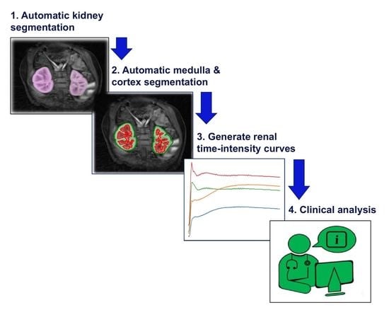
- The improved segmentation of internal kidney regions could provide an opportunity to explore large-scale time–intensity curves of the medulla and cortex and, in doing so, could allow radiologists to differentiate clinically “normal” kidneys from conditions caused by obstruction of urine flow and dilation of the ureter.
2. Materials and Methods
2.1. Data
2.2. Automatic Kidney Segmentation
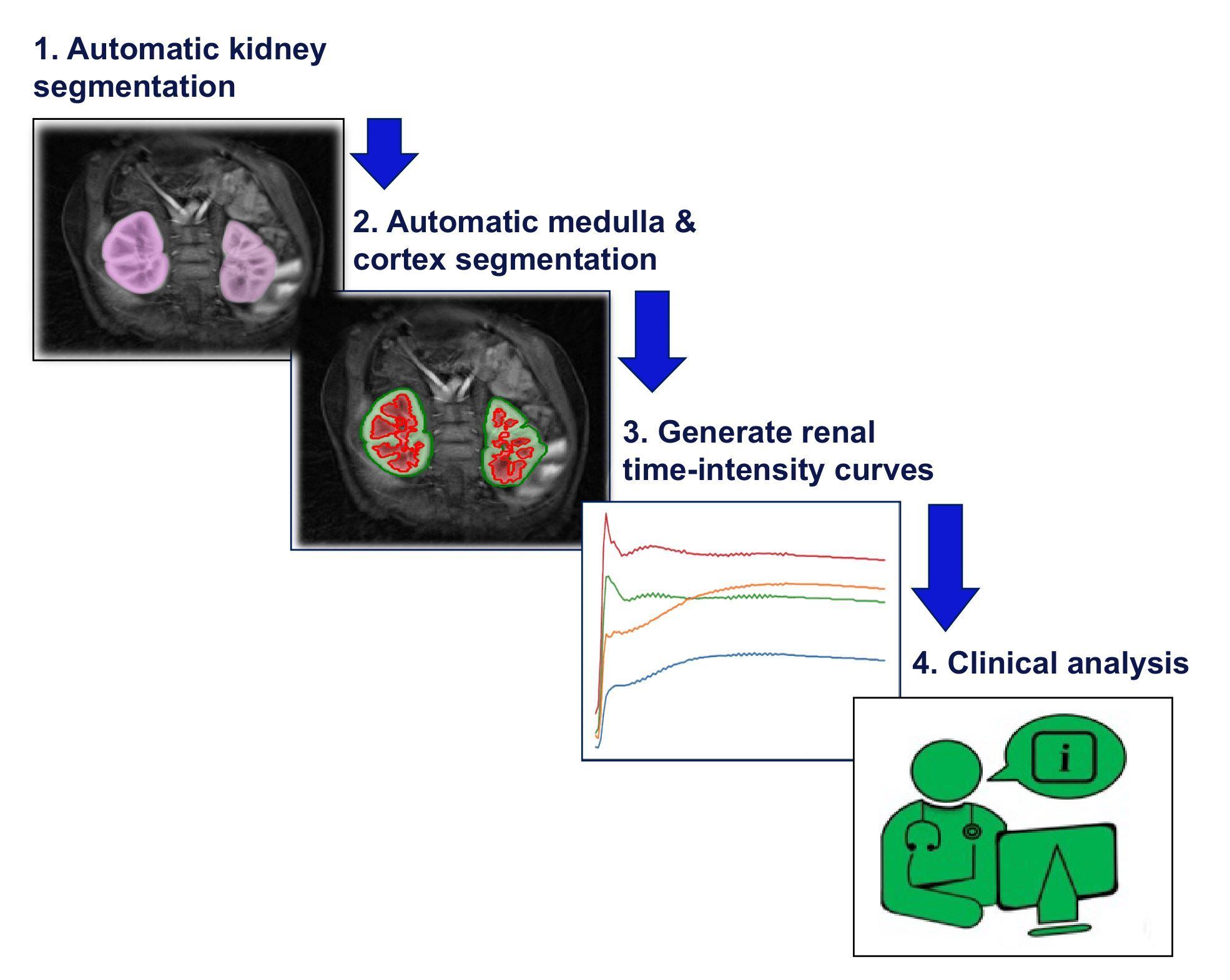
2.2.1. Training Stage
Detection and Localisation
Segmentation
2.2.2. Testing Stage
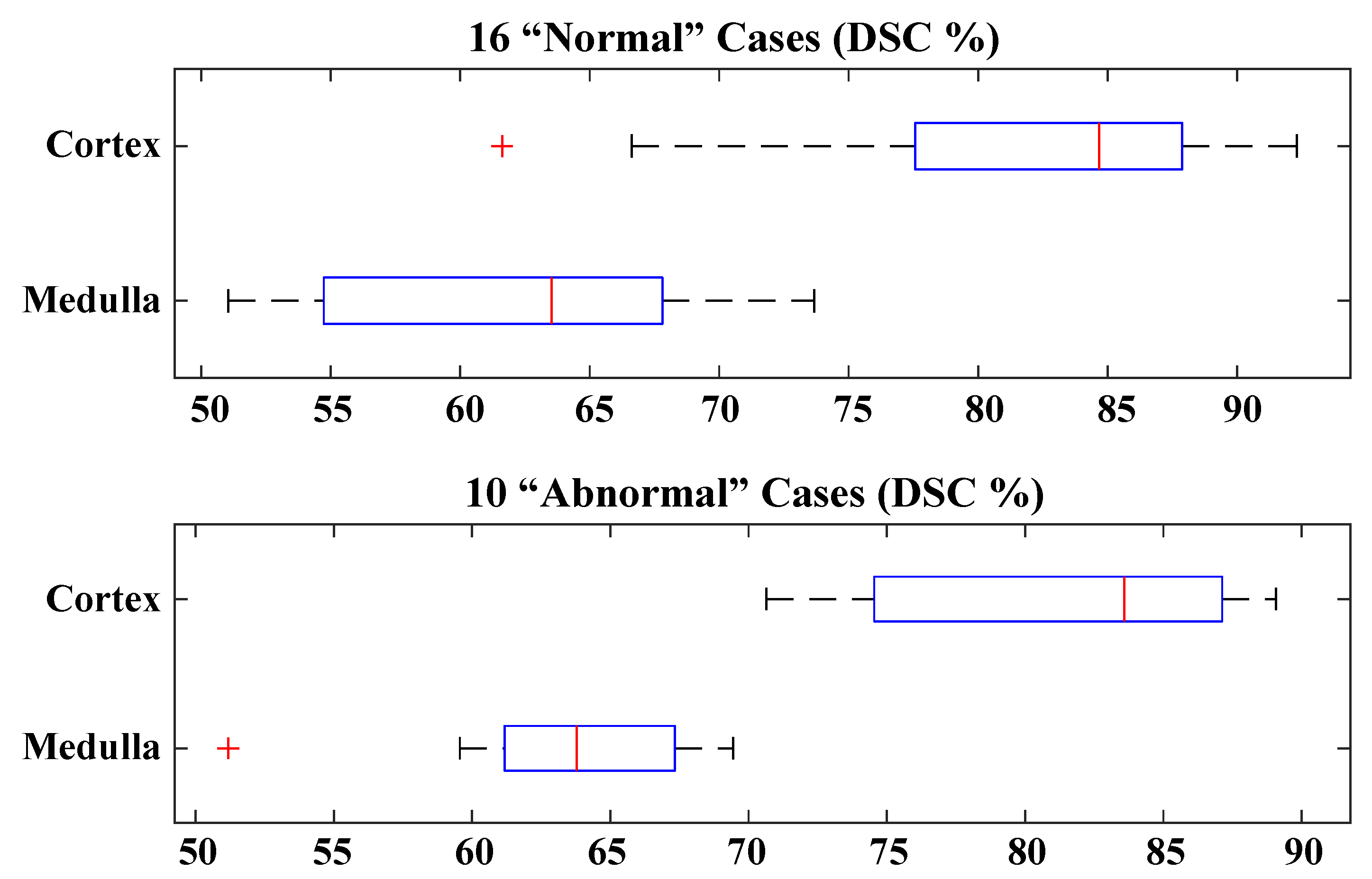
2.3. Automatic Medulla and Cortex Segmentation
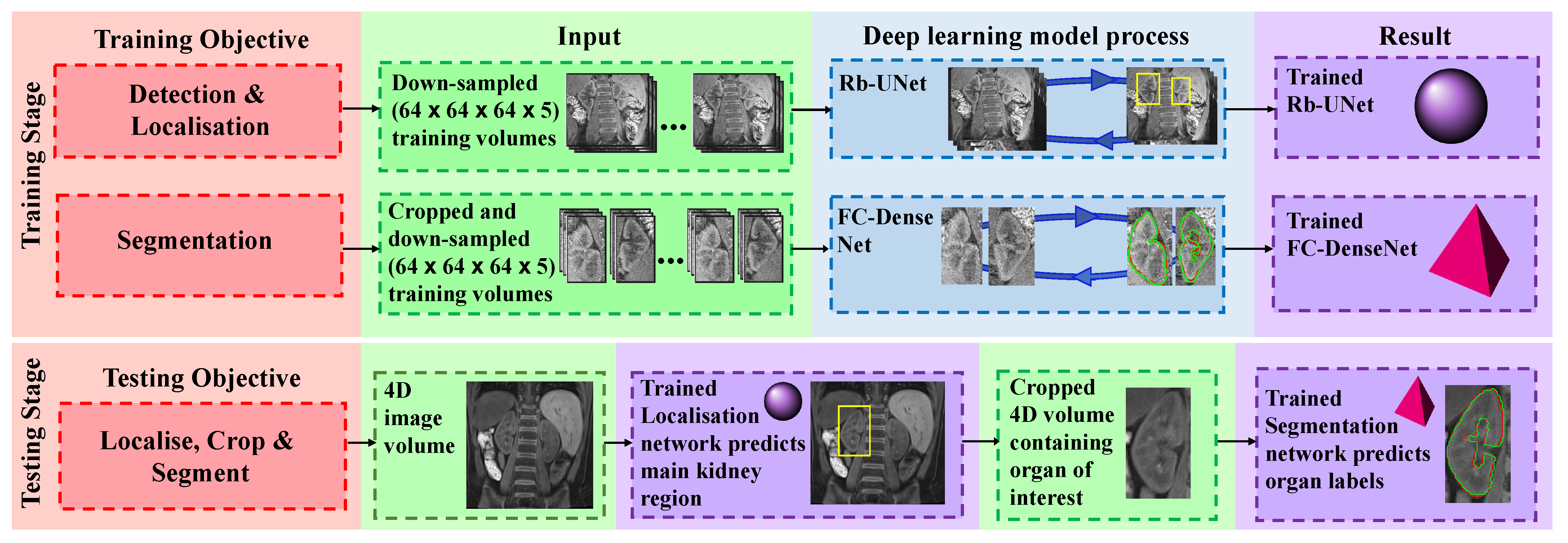
| Algorithm 1: Medulla and Cortex Segmentation Process |
Data: DCE-MRI scan as a sequence of T 3D volumes: , where and H is the height, W is the width and D is the depth of each volume; Threshold parameters: (gain), (cut-off), (gamma correction); Range parameters: , ; Whole-kidney segmented binary mask: where . Result: 3D volume segmentation mask of the medulla and cortex in the whole kidney: , where . Process 1: Establish if the right kidney exists and if left kidney exists. Process 2: Segment the medulla and cortex for all 3D volumes in V from to . Process 3: Fuse the “optimum” medulla and cortex from all segmentations over time, to , into the final medulla and cortex 3D volume. |
2.3.1. Segmenting the Medulla and Cortex for All 3D Volumes in 4D DCE-MRI
- The segmented binary mask of the kidney from Section 2.2 is defined as , where , as shown in Figure 2, Process 2(d). Here, a 2D image, , is fully closed to obtain , as shown in Figure 2, Process 2(e).
- Possible false positives in are eliminated by updating the background in to the same background as in , as shown in Figure 2, Process 2(f).
- If the initial pixel value is 0 and 1 in and , respectively, then this pixel is labelled as “medulla”, as shown in dark grey in Figure 2, Process 2(g). Otherwise, this pixel is labelled as “cortex”.
2.3.2. Generating the “Optimum” Medulla and Cortex 3D Volume
- Total area where as .
- Medulla area in as .
- Percentage of medulla in total kidney area, .
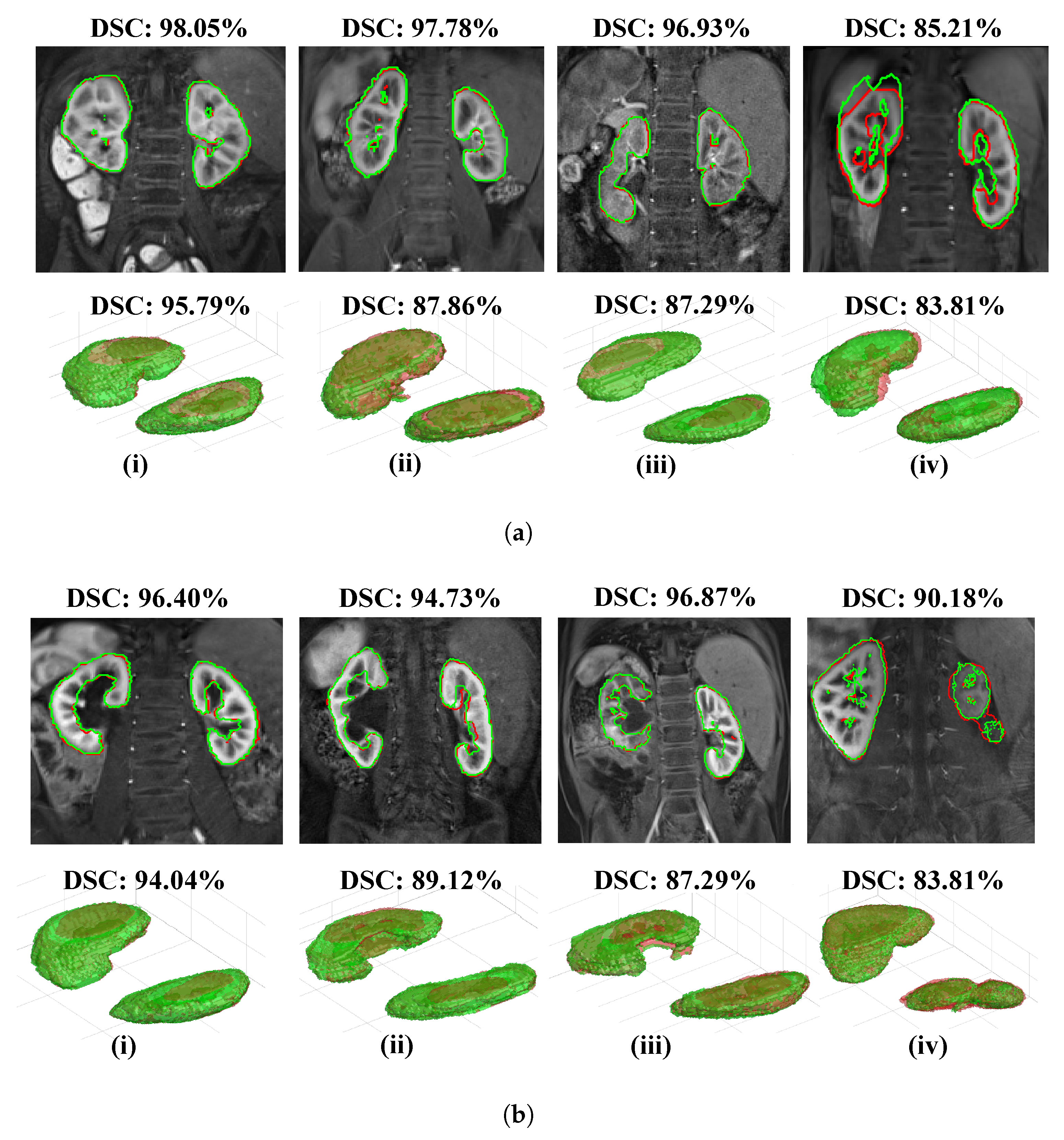
3. Results
3.1. Experimental Setup
Evaluation
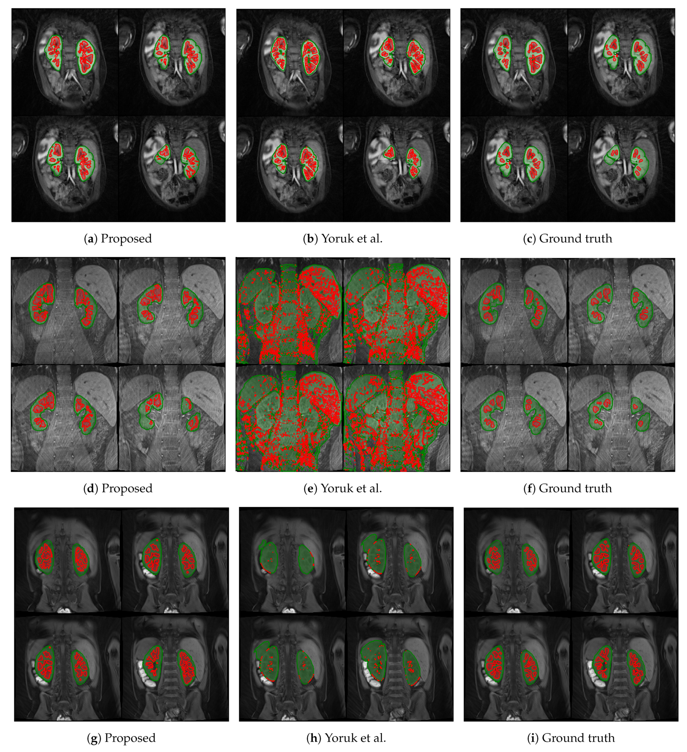
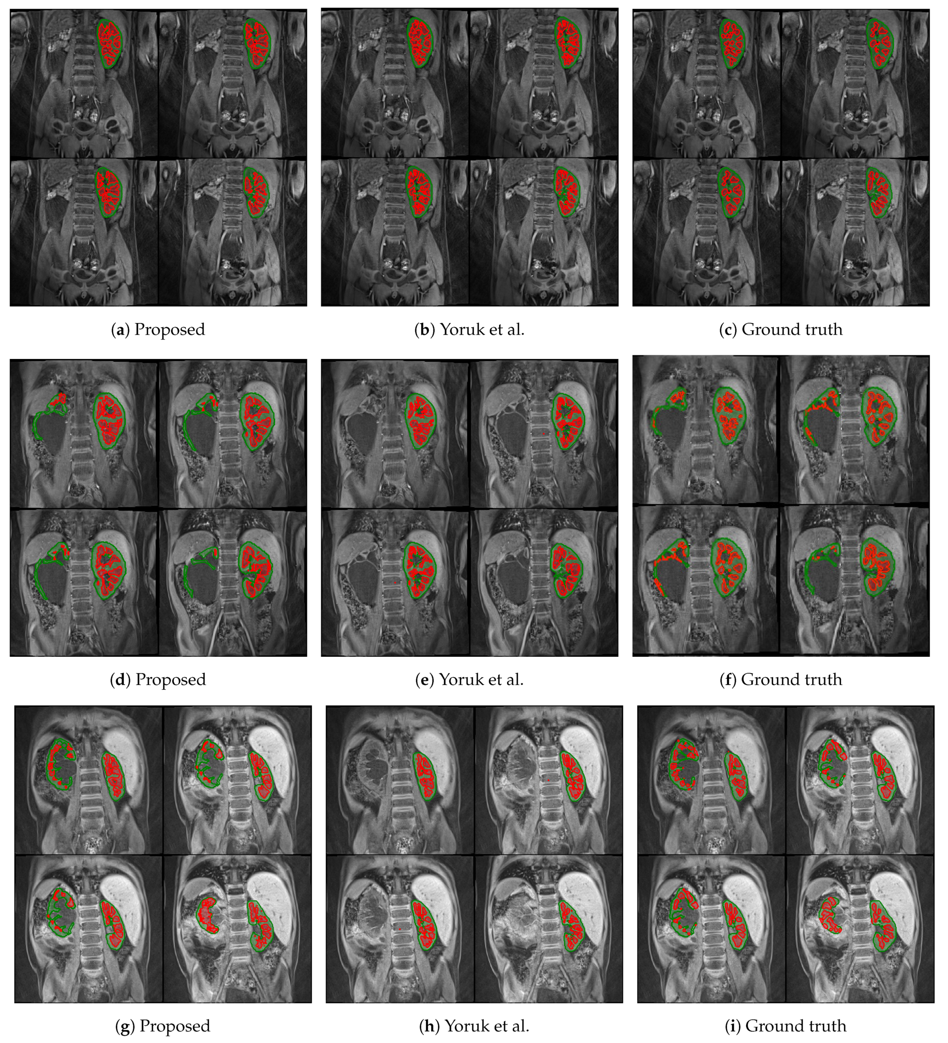
3.2. Renal Segmentation
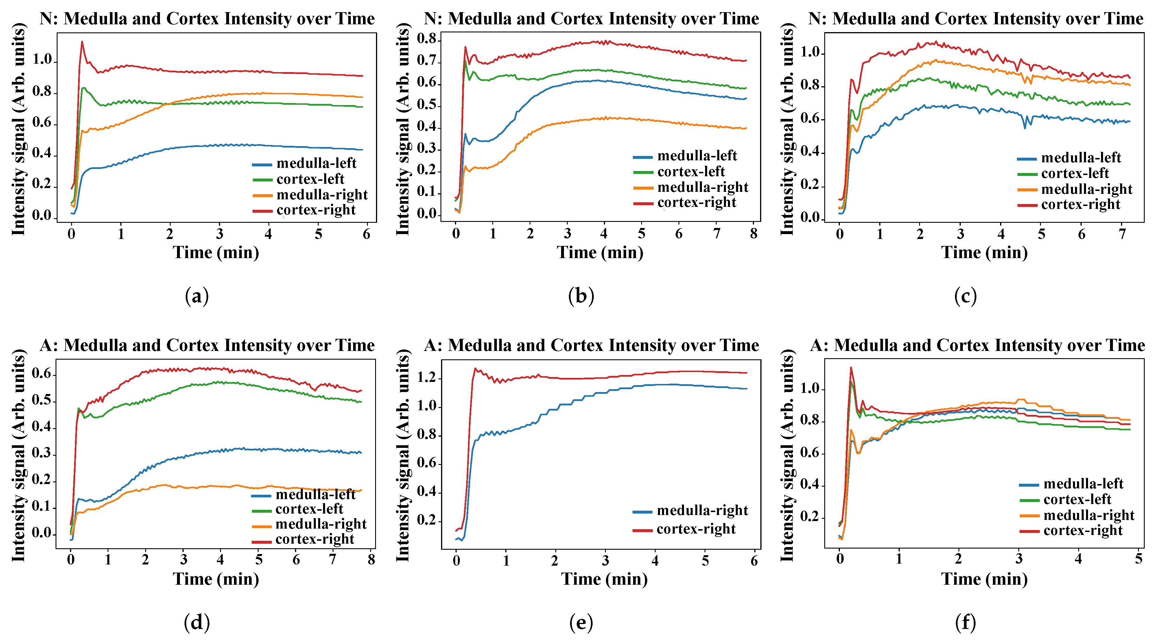
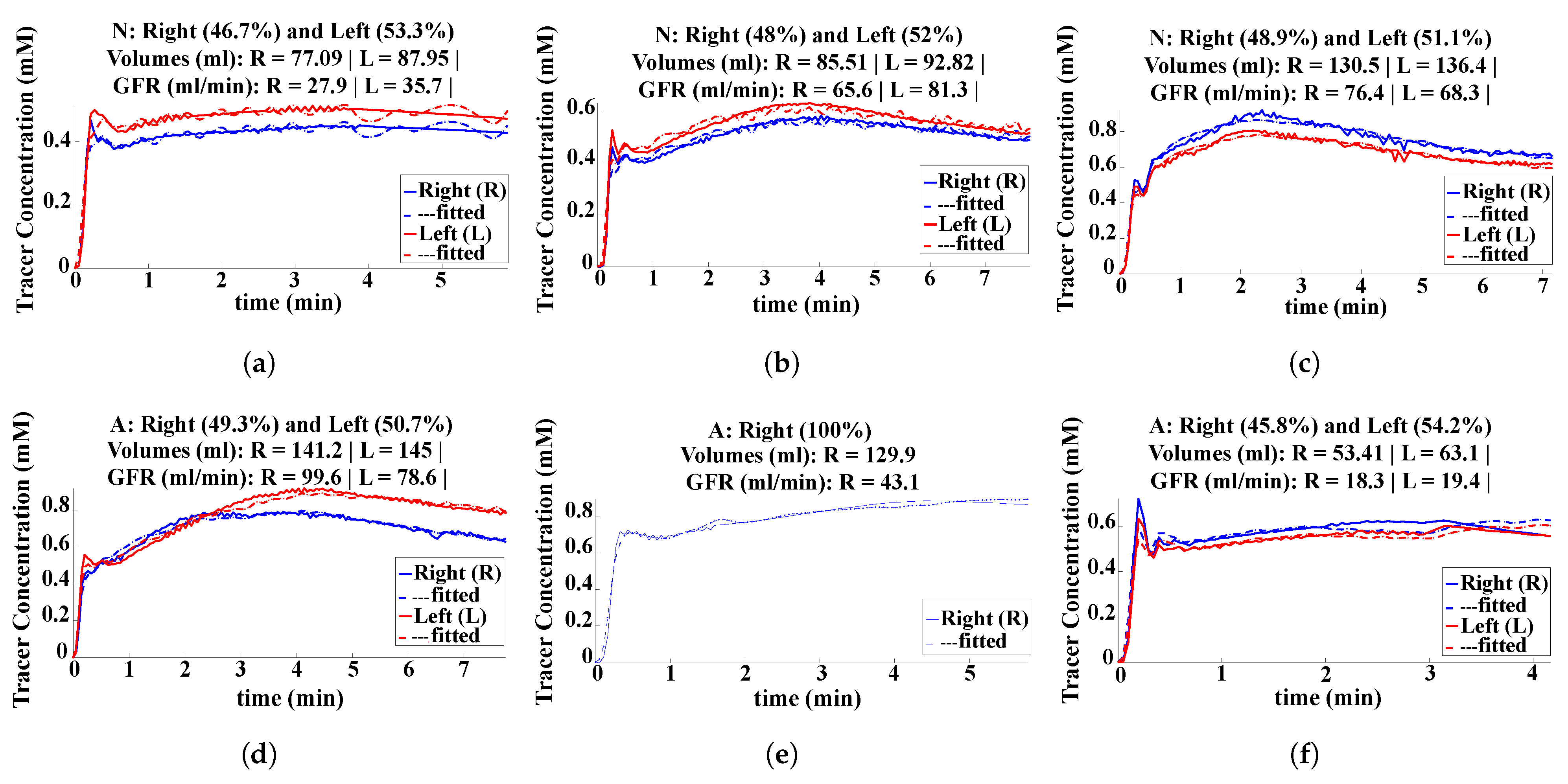
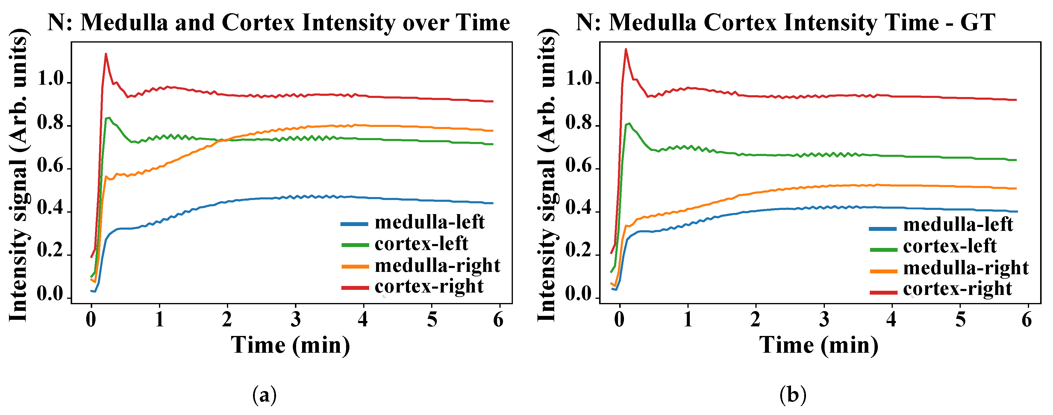
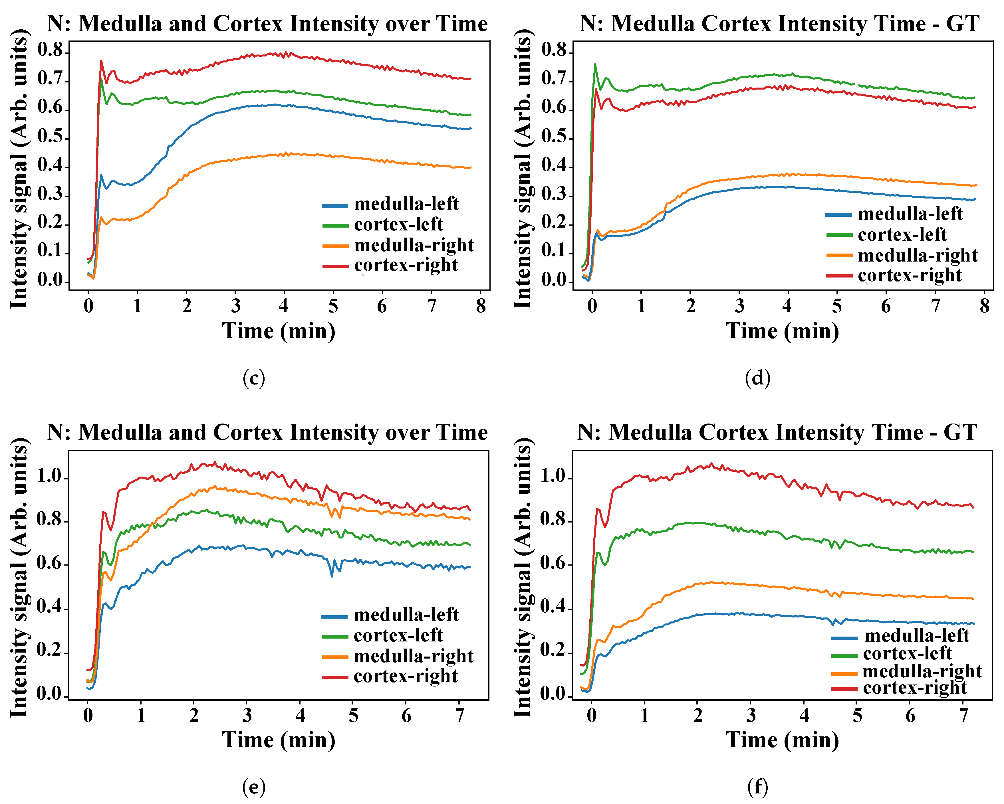
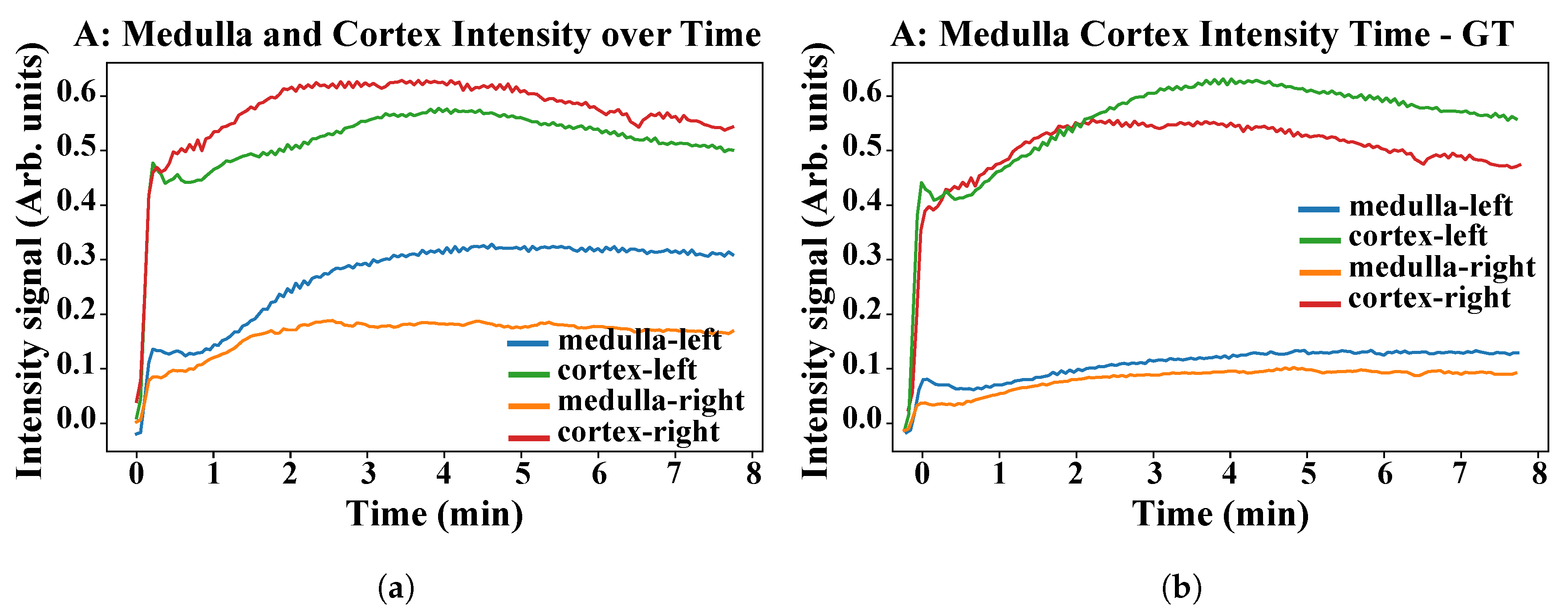
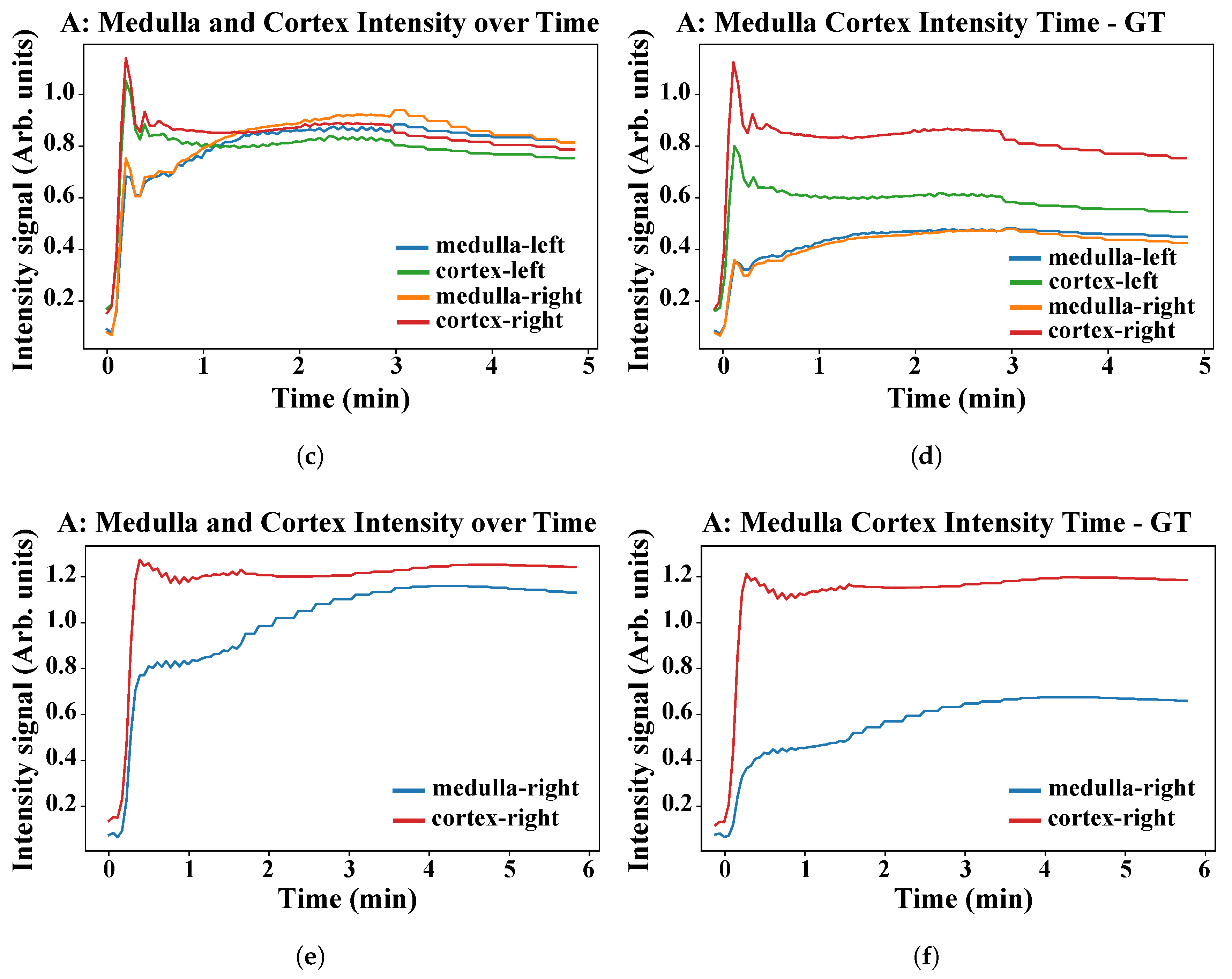
Time–Intensity and Tracer Concentration Curves
4. Discussion
Application
5. Conclusions
Author Contributions
Funding
Institutional Review Board Statement
Informed Consent Statement
Acknowledgments
Conflicts of Interest
Appendix A


References
- Raimann, J.G.; Riella, M.C.; Levin, N.W. International Society of Nephrology’s oby25 initiative (zero preventable deaths from acute kidney injury by 2025): Focus on diagnosis of acute kidney injury in low-income countries. Clin. Kidney J. 2018, 11, 12–19. [Google Scholar] [CrossRef] [PubMed]
- Cohen, S.D.; Davison, S.N.; Kimmel, P.L. Pain and Chronic Kidney Disease. In Chronic Renal Disease; Elsevier: Amsterdam, The Netherlands, 2020; pp. 1279–1289. [Google Scholar]
- Ebrahimi, B.; Textor, S.C.; Lerman, L.O. Renal relevant radiology: Renal functional magnetic resonance imaging. Clin. J. Am. Soc. Nephrol. 2014, 9, 395–405. [Google Scholar] [CrossRef] [PubMed] [Green Version]
- Asaturyan, H.; Thomas, E.L.; Bell, J.D.; Villarini, B. A Framework for Automatic Morphological Feature Extraction and Analysis of Abdominal Organs in MRI Volumes. J. Med Syst. 2019, 43, 334. [Google Scholar] [CrossRef] [PubMed] [Green Version]
- Gounden, V.; Jialal, I. Renal Function Tests; StatPearls Publishing: Treasure Island, FL, USA, 2019. [Google Scholar]
- Thurman, J.M.; Gueler, F. Recent advances in renal imaging. F1000Research 2018, 7, F1000. [Google Scholar] [CrossRef] [Green Version]
- Kong, H.; Chen, B.; Zhang, X.; Wang, C.; Yang, M.; Yang, L.; Wang, X.; Zhang, J. Quantitative renal function assessment of atheroembolic renal disease using view-shared compressed sensing based dynamic-contrast enhanced MR imaging: An in vivo study. Magn. Reson. Imaging 2020, 65, 67–74. [Google Scholar] [CrossRef]
- Kurugol, S.; Afacan, O.; Lee, R.S.; Seager, C.M.; Ferguson, M.A.; Stein, D.R.; Nichols, R.C.; Dugan, M.; Stemmer, A.; Warfield, S.K.; et al. Prospective pediatric study comparing glomerular filtration rate estimates based on motion-robust dynamic contrast-enhanced magnetic resonance imaging and serum creatinine (eGFR) to 99m Tc DTPA. Pediatr. Radiol. 2020, 50, 698–705. [Google Scholar] [CrossRef]
- Kurugol, S.; Seager, C.; Thaker, H.; Coll-Font, J.; Afacan, O.; Nichols, R.; Warfield, S.; Lee, R.; Chow, J. Feed and wrap magnetic resonance urography provides anatomic and functional imaging in infants without anesthesia. J. Pediatr. Urol. 2020, 16, 116–120. [Google Scholar] [CrossRef]
- Coll-Font, J.; Afacan, O.; Chow, J.S.; Lee, R.S.; Stemmer, A.; Warfield, S.K.; Kurugol, S. Bulk motion-compensated DCE-MRI for functional imaging of kidneys in newborns. J. Magn. Reson. Imaging 2020, 52, 207–216. [Google Scholar] [CrossRef]
- Nguyen, H.T.; Herndon, C.A.; Cooper, C.; Gatti, J.; Kirsch, A.; Kokorowski, P.; Lee, R.; Perez-Brayfield, M.; Metcalfe, P.; Yerkes, E.; et al. The Society for Fetal Urology consensus statement on the evaluation and management of antenatal hydronephrosis. J. Pediatr. Urol. 2010, 6, 212–231. [Google Scholar] [CrossRef]
- Zöllner, F.G.; Svarstad, E.; Munthe-Kaas, A.Z.; Schad, L.R.; Lundervold, A.; Rørvik, J. Assessment of kidney volumes from MRI: Acquisition and segmentation techniques. Am. J. Roentgenol. 2012, 199, 1060–1069. [Google Scholar] [CrossRef]
- Eikefjord, E.; Andersen, E.; Hodneland, E.; Zöllner, F.; Lundervold, A.; Svarstad, E.; Rørvik, J. Use of 3D DCE-MRI for the estimation of renal perfusion and glomerular filtration rate: An intrasubject comparison of FLASH and KWIC with a comprehensive framework for evaluation. Am. J. Roentgenol. 2015, 204, W273–W281. [Google Scholar] [CrossRef] [PubMed] [Green Version]
- Haghighi, M.; Warfield, S.K.; Kurugol, S. Automatic renal segmentation in DCE-MRI using convolutional neural networks. In Proceedings of the 2018 IEEE 15th International Symposium on Biomedical Imaging (ISBI 2018), Washington, DC, USA, 4–7 April 2018; pp. 1534–1537. [Google Scholar]
- Villarini, B.; Asaturyan, H.; Kurugol, S.; Afacan, O.; Bell, J.D.; Thomas, E.L. 3D Deep Learning for Anatomical Structure Segmentation in Multiple Imaging Modalities. In Proceedings of the 2021 IEEE 34th International Symposium on Computer-Based Medical Systems (CBMS), Online, 7–9 June 2021; pp. 166–171. [Google Scholar]
- Yoruk, U.; Hargreaves, B.A.; Vasanawala, S.S. Automatic renal segmentation for MR urography using 3D-GrabCut and random forests. Magn. Reson. Med. 2018, 79, 1696–1707. [Google Scholar] [CrossRef]
- Chevaillier, B.; Ponvianne, Y.; Collette, J.L.; Mandry, D.; Claudon, M.; Pietquin, O. Functional semi-automated segmentation of renal DCE-MRI sequences. In Proceedings of the 2008 IEEE International Conference on Acoustics, Speech and Signal Processing, Las Vegas, NV, USA, 31 March–4 April 2008; pp. 525–528. [Google Scholar]
- Huang, W.; Li, H.; Wang, R.; Zhang, X.; Wang, X.; Zhang, J. A self-supervised strategy for fully automatic segmentation of renal dynamic contrast-enhanced magnetic resonance images. Med Phys. 2019, 46, 4417–4430. [Google Scholar] [CrossRef]
- Yang, X.; Le Minh, H.; Cheng, K.T.T.; Sung, K.H.; Liu, W. Renal compartment segmentation in DCE-MRI images. Med. Image Anal. 2016, 32, 269–280. [Google Scholar] [CrossRef] [PubMed]
- Donoser, M.; Bischof, H. 3d segmentation by maximally stable volumes (msvs). In Proceedings of the 18th International Conference on Pattern Recognition (ICPR’06), Hong Kong, China, 20–24 August 2006; Volume 1, pp. 63–66. [Google Scholar]
- Boykov, Y.; Funka-Lea, G. Graph cuts and efficient ND image segmentation. Int. J. Comput. Vis. 2006, 70, 109–131. [Google Scholar] [CrossRef] [Green Version]
- Feng, L.; Grimm, R.; Block, K.T.; Chandarana, H.; Kim, S.; Xu, J.; Axel, L.; Sodickson, D.K.; Otazo, R. Golden-angle radial sparse parallel MRI: Combination of compressed sensing, parallel imaging, and golden-angle radial sampling for fast and flexible dynamic volumetric MRI. Magn. Reson. Med. 2014, 72, 707–717. [Google Scholar] [CrossRef] [Green Version]
- He, K.; Zhang, X.; Ren, S.; Sun, J. Deep residual learning for image recognition. In Proceedings of the IEEE Conference on Computer Vision and Pattern Recognition, Las Vegas, NV, USA, 27 June–1 July 2016; pp. 770–778. [Google Scholar]
- Ronneberger, O.; Fischer, P.; Brox, T. U-Net: Convolutional Networks for Biomedical Image Segmentation. In Proceedings of the MICCAI 2015, Munich, Germany, 5–9 October 2015; Springer International Publishing: New York, NY, USA, 2015; pp. 234–241. [Google Scholar]
- Huang, G.; Liu, Z.; Van Der Maaten, L.; Weinberger, K.Q. Densely connected convolutional networks. In Proceedings of the IEEE Conference on Computer Vision and Pattern Recognition, Honolulu, HI, USA, 21–26 July 2017; pp. 4700–4708. [Google Scholar]
- Çiçek, Ö.; Abdulkadir, A.; Lienkamp, S.S.; Brox, T.; Ronneberger, O. 3D U-Net: Learning dense volumetric segmentation from sparse annotation. In Proceedings of the International Conference on Medical Image Computing and Computer-Assisted Intervention, Athens, Greece, 17–21 October 2016; pp. 424–432. [Google Scholar]
- Jégou, S.; Drozdzal, M.; Vazquez, D.; Romero, A.; Bengio, Y. The one hundred layers tiramisu: Fully convolutional densenets for semantic segmentation. In Proceedings of the IEEE Conference on Computer Vision and Pattern Recognition Workshops, Honolulu, HI, USA, 21–26 July 2017; pp. 11–19. [Google Scholar]
- Abdi, H.; Williams, L.J. Principal component analysis. Wiley Interdiscip. Rev. Comput. Stat. 2010, 2, 433–459. [Google Scholar] [CrossRef]
- Asaturyan, H.; Gligorievski, A.; Villarini, B. Morphological and multi-level geometrical descriptor analysis in CT and MRI volumes for automatic pancreas segmentation. Comput. Med. Imaging Graph. 2019, 75, 1–13. [Google Scholar] [CrossRef]
- Bangare, S.L.; Dubal, A.; Bangare, P.S.; Patil, S. Reviewing Otsu’s method for image thresholding. Int. J. Appl. Eng. Res. 2015, 10, 21777–21783. [Google Scholar] [CrossRef]
- Kingma, D.P.; Ba, J. Adam: A method for stochastic optimization. arXiv 2014, arXiv:1412.6980. [Google Scholar]
- Milletari, F.; Navab, N.; Ahmadi, S.A. V-net: Fully convolutional neural networks for volumetric medical image segmentation. In Proceedings of the 2016 Fourth International Conference on 3D Vision (3DV), Stanford, CA, USA, 25–28 October 2016; pp. 565–571. [Google Scholar]
- Wu, Z.; Hai, J.; Zhang, L.; Chen, J.; Cheng, G.; Yan, B. Cascaded Fully Convolutional DenseNet for Automatic Kidney Segmentation in Ultrasound Images. In Proceedings of the 2019 2nd International Conference on Artificial Intelligence and Big Data (ICAIBD), Chengdu, China, 25–28 May 2019; pp. 384–388. [Google Scholar]
- Yoruk, U.; Hargreaves, B.A.; Vasanawala, S.S. Automatic Renal Segmentation for MR Urography Using 3D-GrabCut and Random Forests. 2018. Available online: https://github.com/umityoruk/renal-segmentation (accessed on 26 April 2020).
- Sivakumar, V.N.; Indiran, V.; Sathyanathan, B.P. Dynamic MRI and isotope renogram in the functional evaluation of pelviureteric junction obstruction: A comparative study. Turk. J. Urol. 2018, 44, 45. [Google Scholar] [CrossRef] [PubMed] [Green Version]
- Floege, J.; Johnson, R.J.; Feehally, J. Comprehensive Clinical Nephrology E-Book; Elsevier Health Sciences: Amsterdam, The Netherlands, 2010. [Google Scholar]
- Sourbron, S.P.; Michaely, H.J.; Reiser, M.F.; Schoenberg, S.O. MRI measurement of perfusion and glomerular filtration in the human kidney with a separable compartment model. Investig. Radiol. 2008, 43, 40–48. [Google Scholar] [CrossRef] [PubMed]
- Tangri, N.; Hougen, I.; Alam, A.; Perrone, R.; McFarlane, P.; Pei, Y. Total kidney volume as a biomarker of disease progression in autosomal dominant polycystic kidney disease. Can. J. Kidney Health Dis. 2017, 4, 2054358117693355. [Google Scholar] [CrossRef] [PubMed] [Green Version]
- Wachs-Lopes, G.A.; Santos, R.M.; Saito, N.; Rodrigues, P.S. Recent nature-Inspired algorithms for medical image segmentation based on tsallis statistics. Commun. Nonlinear Sci. Numer. Simul. 2020, 88, 105256. [Google Scholar] [CrossRef]
- Kallenberg, M.; Petersen, K.; Nielsen, M.; Ng, A.Y.; Diao, P.; Igel, C.; Vachon, C.M.; Holland, K.; Winkel, R.R.; Karssemeijer, N.; et al. Unsupervised deep learning applied to breast density segmentation and mammographic risk scoring. IEEE Trans. Med. Imaging 2016, 35, 1322–1331. [Google Scholar] [CrossRef] [PubMed]
- Moriya, T.; Roth, H.R.; Nakamura, S.; Oda, H.; Nagara, K.; Oda, M.; Mori, K. Unsupervised segmentation of 3D medical images based on clustering and deep representation learning. In Proceedings of the Medical Imaging 2018: Biomedical Applications in Molecular, Structural, and Functional Imaging. International Society for Optics and Photonics, Houston, TX, USA, 11–13 February 2018; Volume 10578, p. 1057820. [Google Scholar]
- Zhang, R.; Isola, P.; Efros, A.A. Split-brain autoencoders: Unsupervised learning by cross-channel prediction. In Proceedings of the IEEE Conference on Computer Vision and Pattern Recognition, Honolulu, HI, USA, 21–26 July 2017; pp. 1058–1067. [Google Scholar]
- Xu, Y.; Du, J.; Dai, L.R.; Lee, C.H. A regression approach to speech enhancement based on deep neural networks. IEEE/ACM Trans. Audio Speech Lang. Process. 2014, 23, 7–19. [Google Scholar] [CrossRef]


| Kidney Condition | Accuracy Result | Proposed Approach | 3D Rb-UNet + 3D U-Net [26] |
|---|---|---|---|
| All | DSC | ||
| PC | |||
| RC | |||
| Normal | DSC | ||
| PC | |||
| RC | |||
| Abnormal | DSC | ||
| PC | |||
| RC |
| Kidney Condition | DCE-MRI Case | Compartment | Proposed | Yoruk et al. [16] |
|---|---|---|---|---|
| Normal | 1 | Medulla | ||
| Cortex | ||||
| 2 | Medulla | |||
| Cortex | ||||
| 3 | Medulla | |||
| Cortex | ||||
| 4 | Medulla | |||
| Cortex | ||||
| 5 | Medulla | |||
| Cortex | ||||
| 6 | Medulla | |||
| Cortex | ||||
| 7 | Medulla | |||
| Cortex | ||||
| 8 | Medulla | |||
| Cortex | ||||
| 9 | Medulla | |||
| Cortex | ||||
| 10 | Medulla | |||
| Cortex | ||||
| 11 | Medulla | |||
| Cortex | ||||
| 12 | Medulla | |||
| Cortex | ||||
| 13 | Medulla | |||
| Cortex | ||||
| 14 | Medulla | |||
| Cortex | ||||
| 15 | Medulla | |||
| Cortex | ||||
| 16 | Medulla | |||
| Cortex | ||||
| Abnormal | 1 | Medulla | ||
| Cortex | ||||
| 2 | Medulla | |||
| Cortex | ||||
| 3 | Medulla | |||
| Cortex | ||||
| 4 | Medulla | |||
| Cortex | ||||
| 5 | Medulla | |||
| Cortex | ||||
| 6 | Medulla | |||
| Cortex | ||||
| 7 | Medulla | |||
| Cortex | ||||
| 8 | Medulla | |||
| Cortex | ||||
| 9 | Medulla | |||
| Cortex | ||||
| 10 | Medulla | |||
| Cortex |
| Compartment | Proposed (%) | Yoruk et al. [16] (%) | |
|---|---|---|---|
| N-16 cases | Cortex | ||
| Medulla | |||
| A-10 cases | Cortex | ||
| Medulla |
Publisher’s Note: MDPI stays neutral with regard to jurisdictional claims in published maps and institutional affiliations. |
© 2021 by the authors. Licensee MDPI, Basel, Switzerland. This article is an open access article distributed under the terms and conditions of the Creative Commons Attribution (CC BY) license (https://creativecommons.org/licenses/by/4.0/).
Share and Cite
Asaturyan, H.; Villarini, B.; Sarao, K.; Chow, J.S.; Afacan, O.; Kurugol, S. Improving Automatic Renal Segmentation in Clinically Normal and Abnormal Paediatric DCE-MRI via Contrast Maximisation and Convolutional Networks for Computing Markers of Kidney Function. Sensors 2021, 21, 7942. https://0-doi-org.brum.beds.ac.uk/10.3390/s21237942
Asaturyan H, Villarini B, Sarao K, Chow JS, Afacan O, Kurugol S. Improving Automatic Renal Segmentation in Clinically Normal and Abnormal Paediatric DCE-MRI via Contrast Maximisation and Convolutional Networks for Computing Markers of Kidney Function. Sensors. 2021; 21(23):7942. https://0-doi-org.brum.beds.ac.uk/10.3390/s21237942
Chicago/Turabian StyleAsaturyan, Hykoush, Barbara Villarini, Karen Sarao, Jeanne S. Chow, Onur Afacan, and Sila Kurugol. 2021. "Improving Automatic Renal Segmentation in Clinically Normal and Abnormal Paediatric DCE-MRI via Contrast Maximisation and Convolutional Networks for Computing Markers of Kidney Function" Sensors 21, no. 23: 7942. https://0-doi-org.brum.beds.ac.uk/10.3390/s21237942