
Localization with Transfer Learning Based on Fine-Grained Subcarrier Information for Dynamic Indoor Environments


Abstract
:1. Introduction
- To overcome the variations in Wi-Fi signals across time, we apply transfer learning to CSI readings for indoor fingerprinting localization.
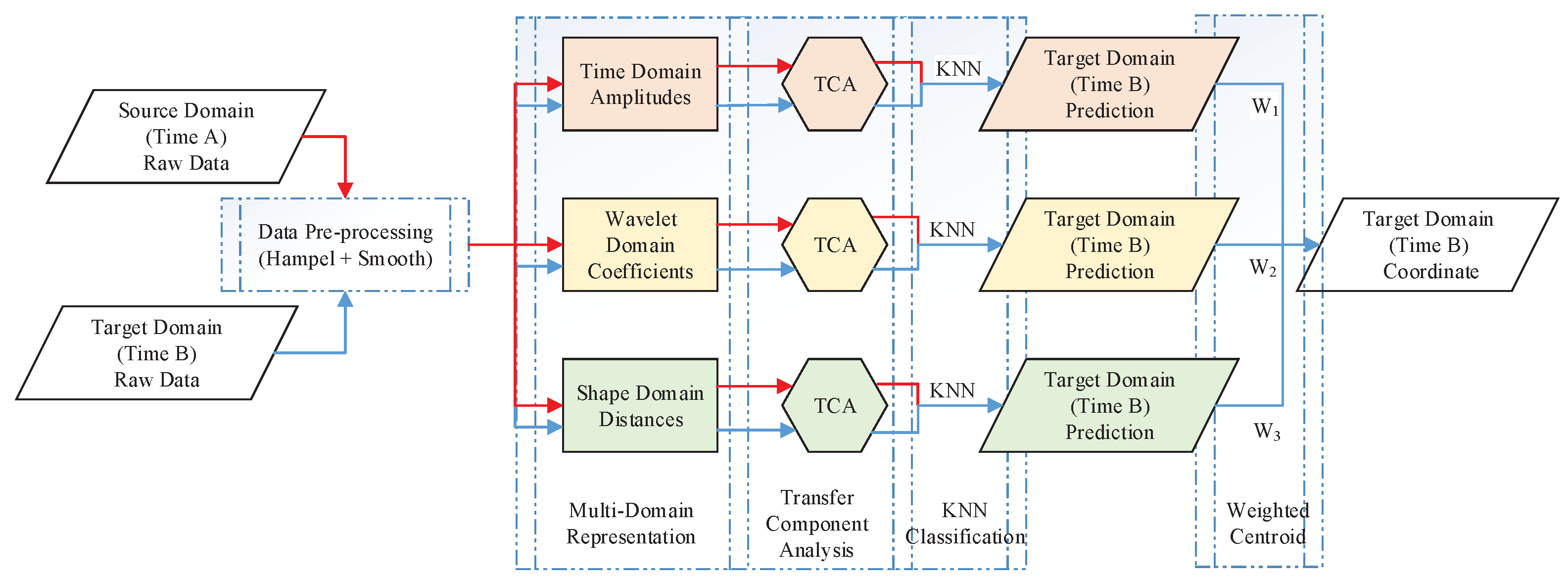
- Unlike using one feature as a fingerprint, we propose three types of CSI feature representations-amplitude in the time domain, wavelet transformations in the frequency domain, and similarity distance in the shape domain-which make full use of the CSI characters in three domains. We also propose a novel strategy utilizing Bayesian model averaging and the weighted centroid algorithm to better fuse the localization results corresponding to the three features.
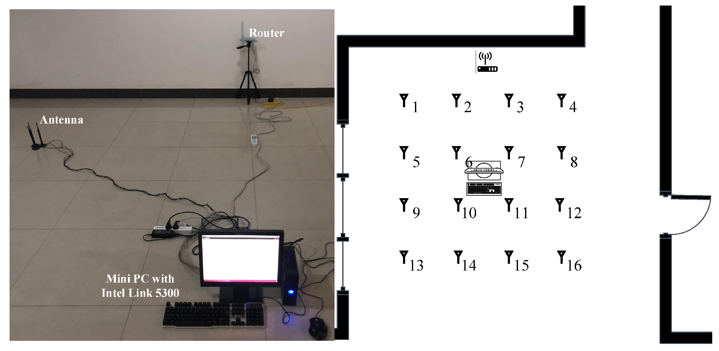
- We collected CSI data from a computer equipped with an Intel WiFi Link 5300 wireless network interface card and conducted two experiments in an open hall and a laboratory. The proposed method’s effectiveness and robustness were verified by comparing the traditional CSI fingerprinting location method with different algorithm parameters.
- We also evaluated our method for the efficiency and validity of localization across several days on a smartphone platform. The experimental results show that the proposed system can achieve performance on a smartphone platform that is comparable with that on the computer platform and is characterized by good robustness.
2. Motivation
2.1. RSSI vs. CSI
2.2. Limitations and Opportunities
3. Methodology
3.1. Data Statement
3.2. Data Preprocessing
3.3. Multi-Domain Representation
3.3.1. Time-Domain Amplitudes
3.3.2. Wavelet-Domain Transformations
3.3.3. Shape-Domain Distances
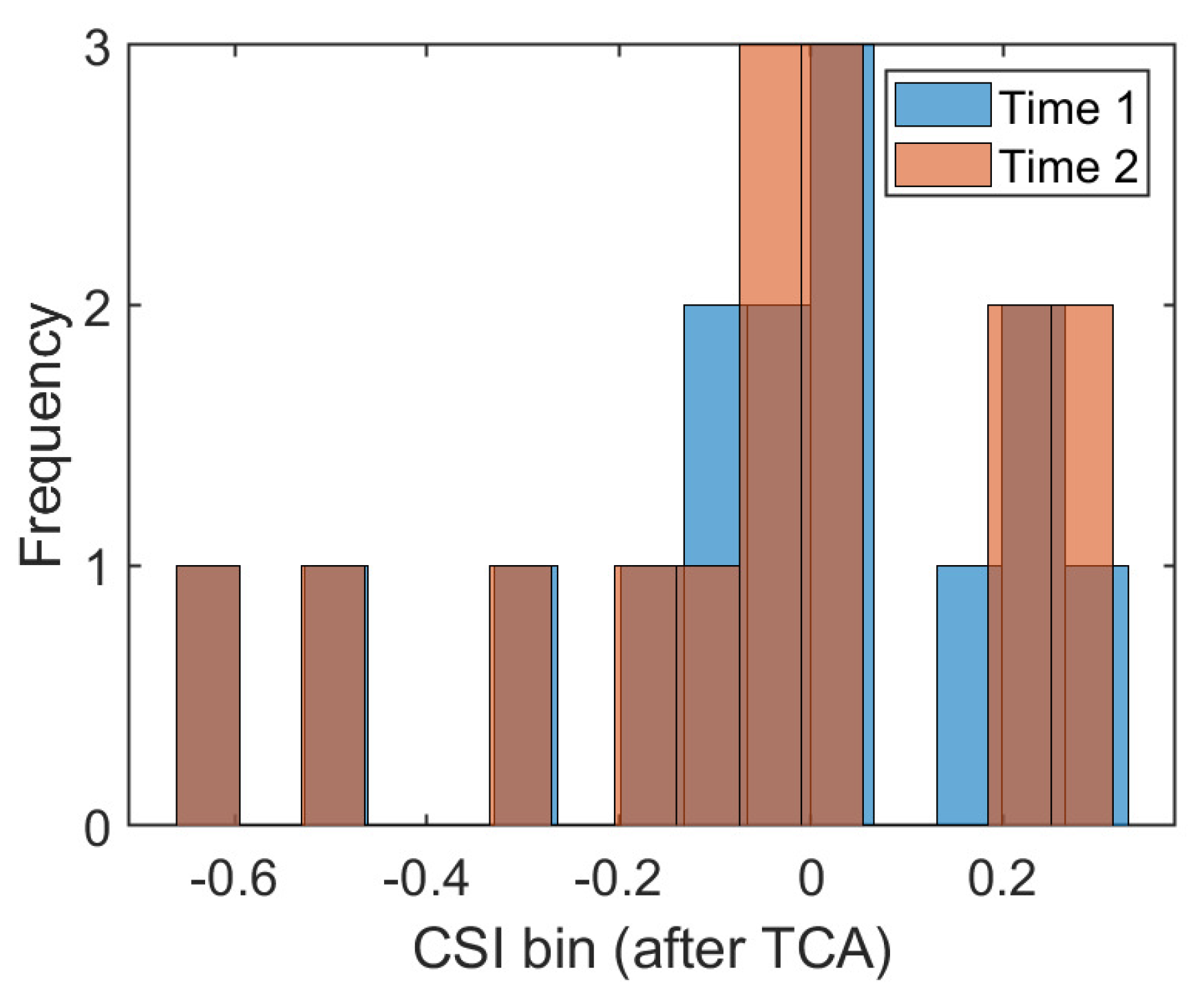
3.4. Transfer Component Analysis
3.5. Label Alignment
3.6. Localization Estimation
4. Experiments
4.1. Experiment 1-Open Hall
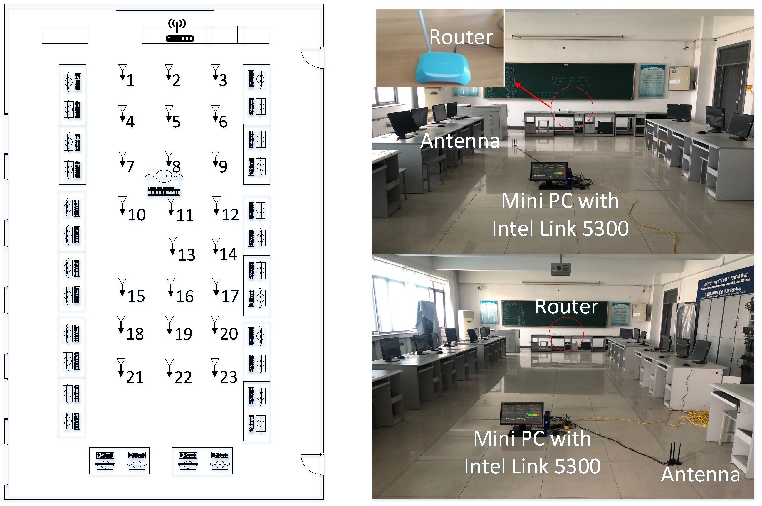
4.1.1. Data Setup
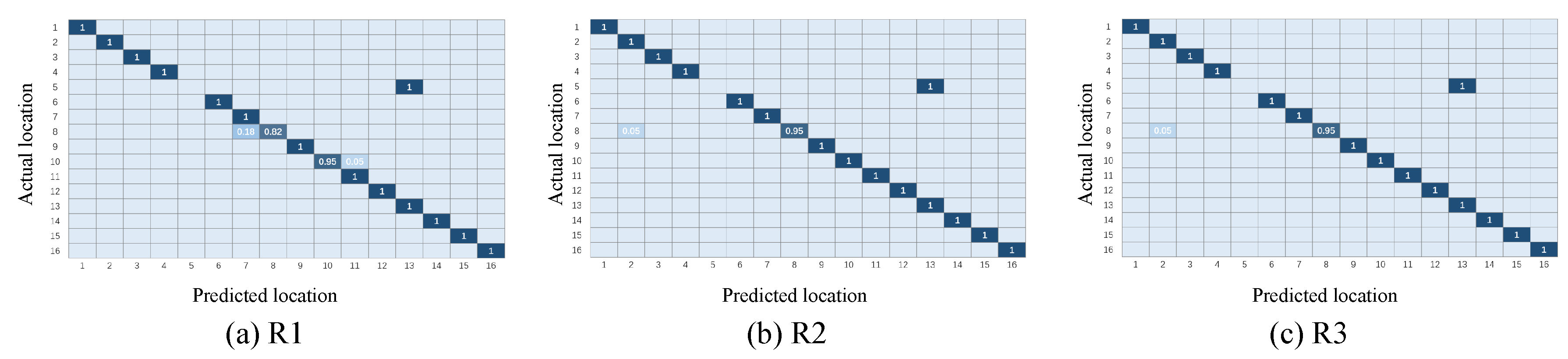
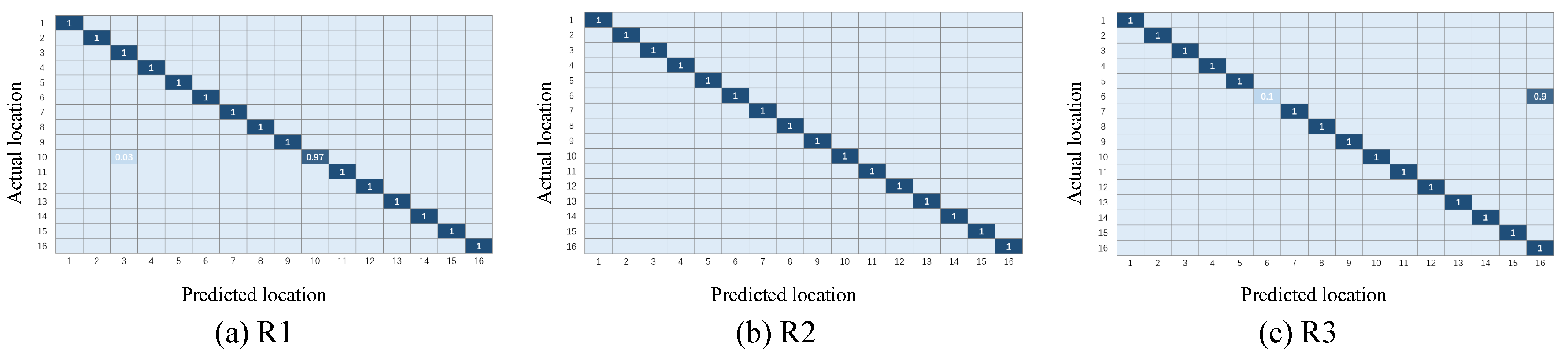
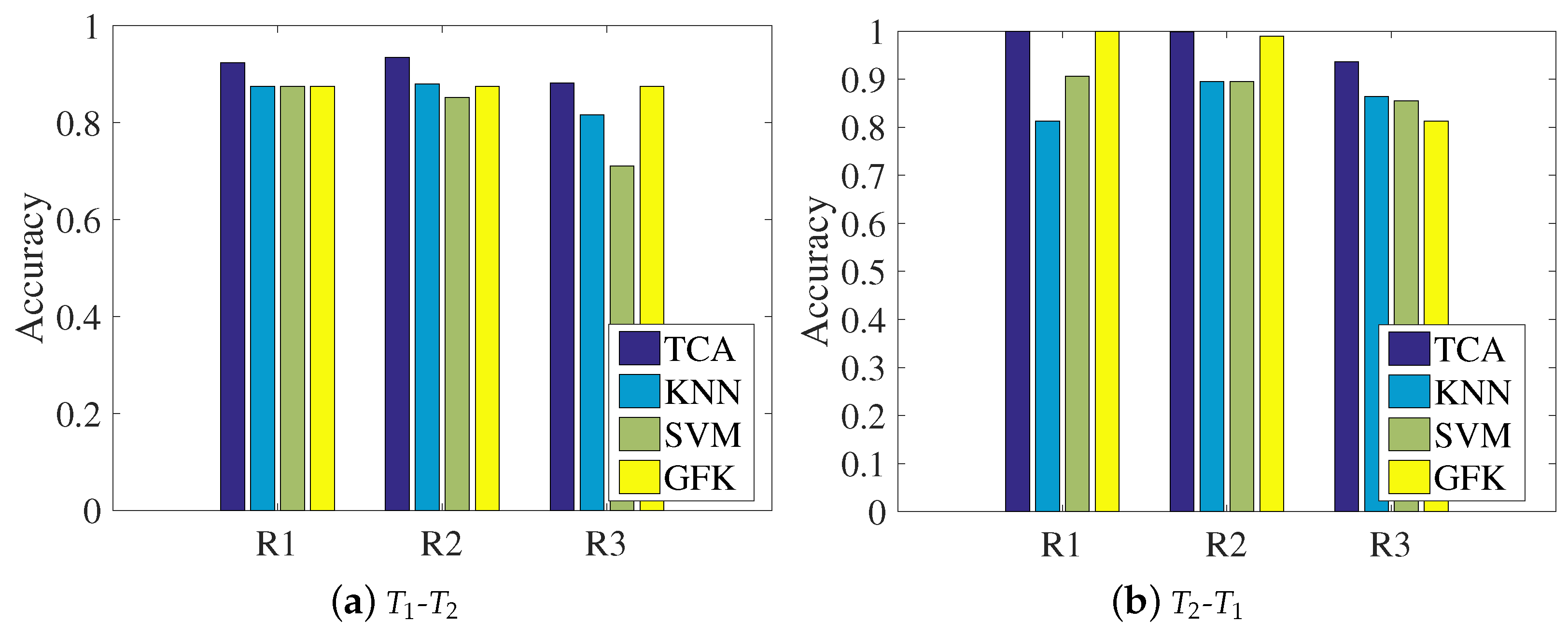
4.1.2. Classification Results of Transfer Learning under Different Representations
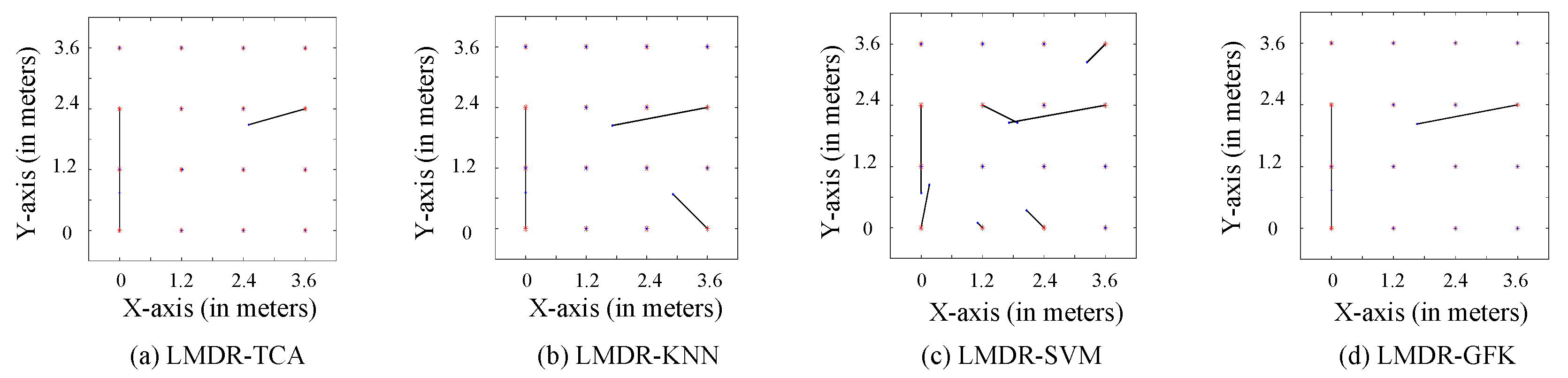
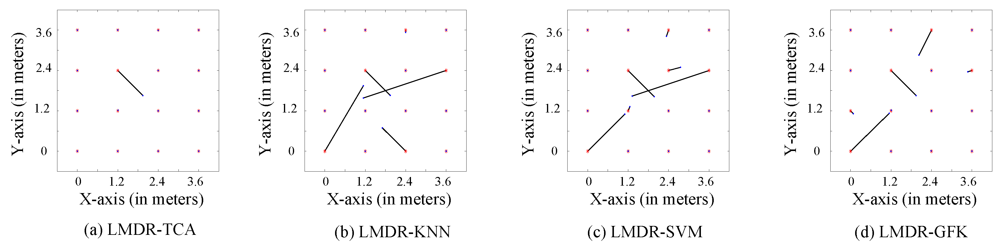
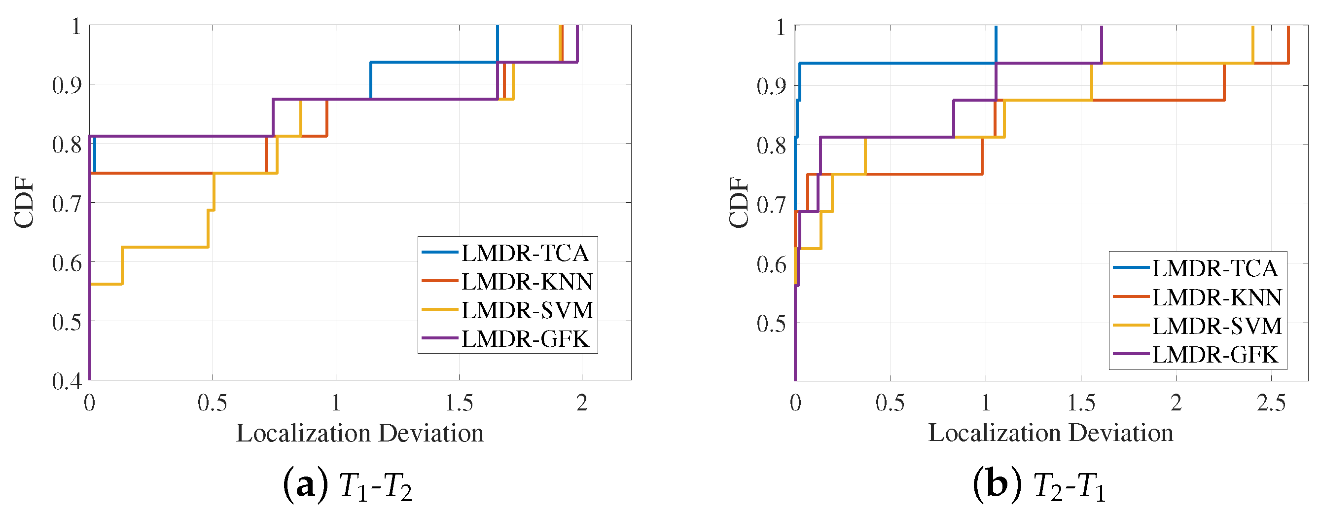
4.1.3. Comparison with Different Methods
4.1.4. Localization Performance under Different Influence Factors
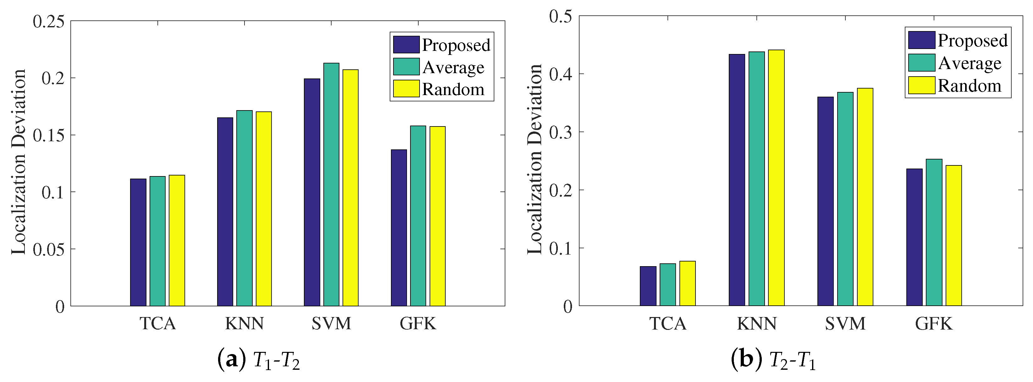
- Impact of the weight coefficient
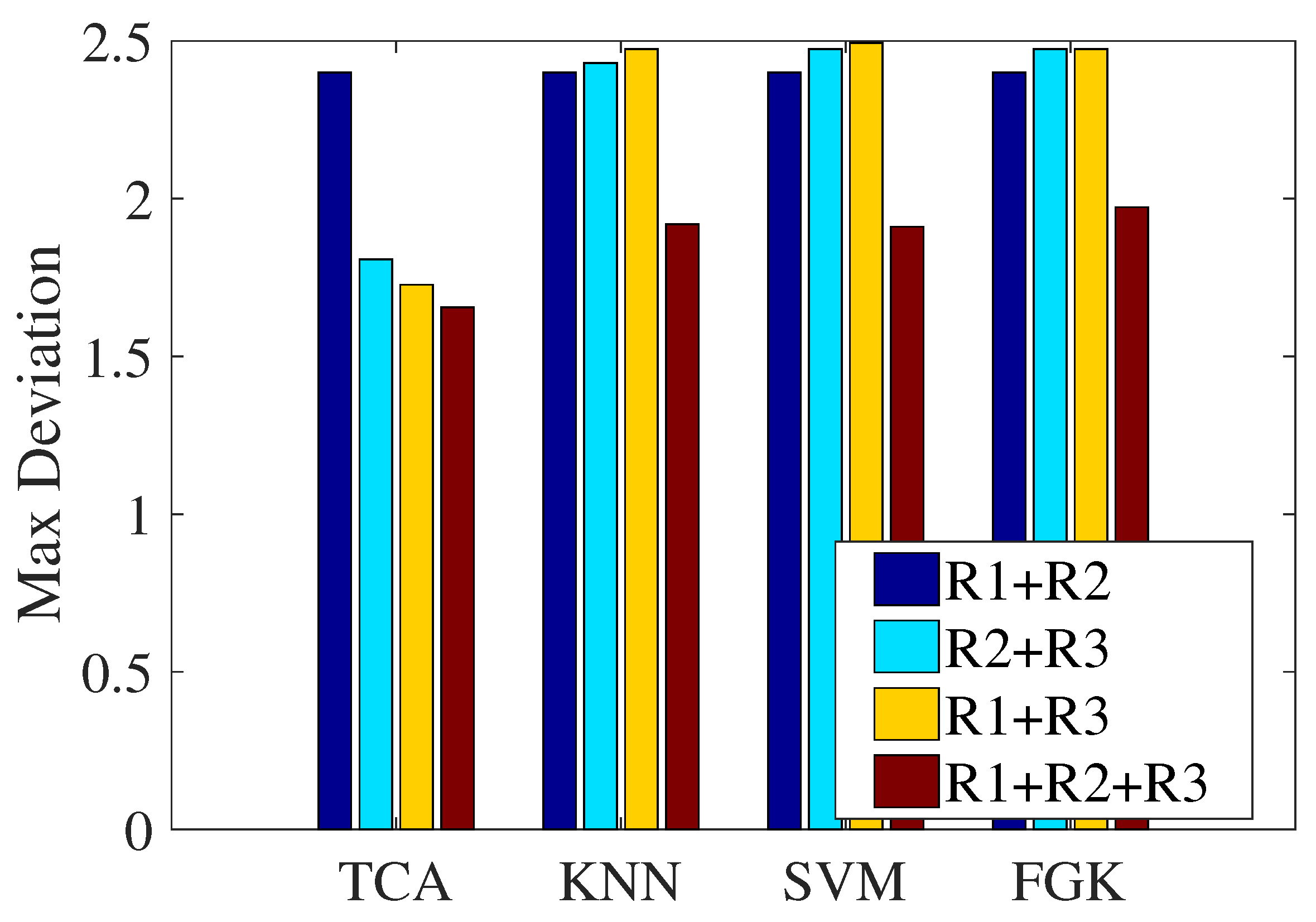
- Impact of the combination of multi-domain representations
4.2. Experiment 2-Closed Laboratory
4.2.1. Setup
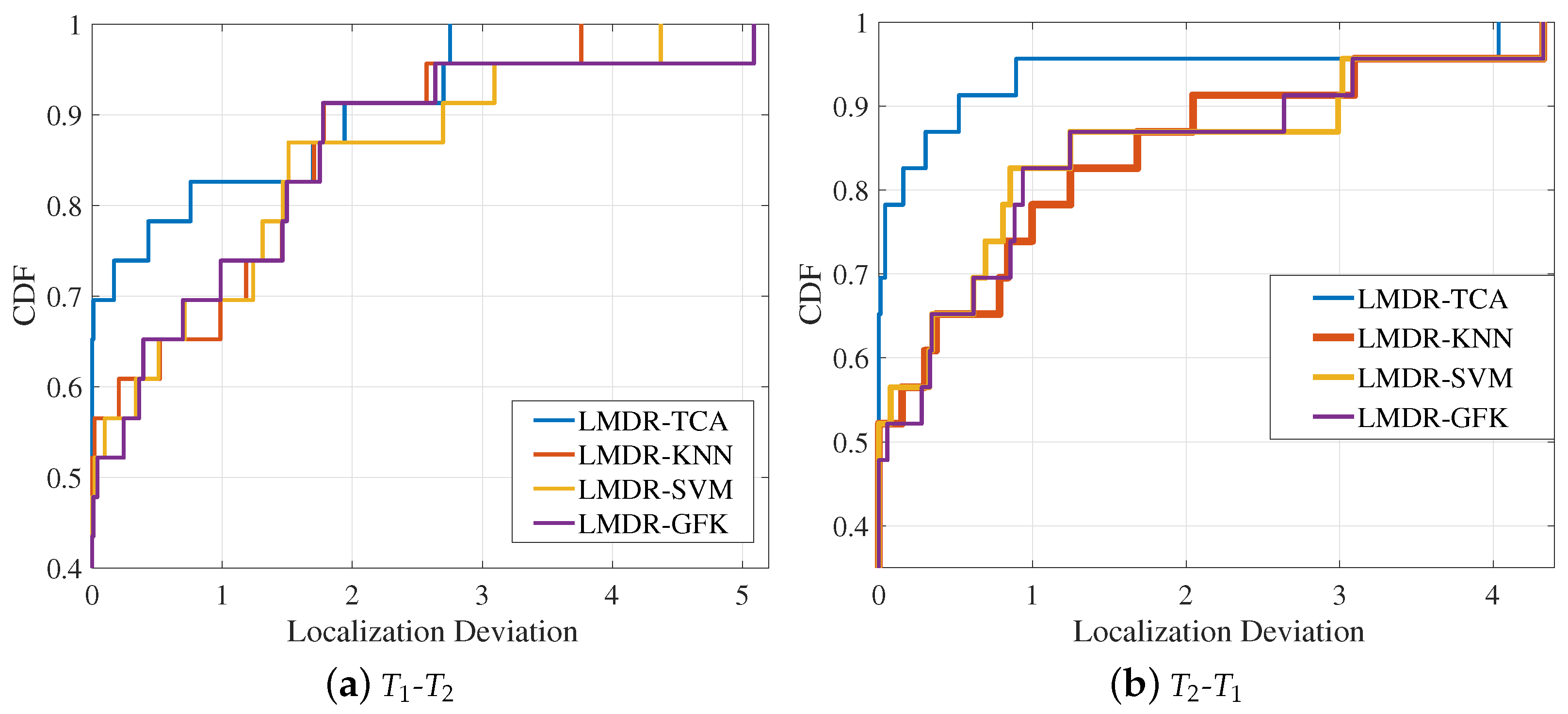
4.2.2. Localization Performance and Comparison
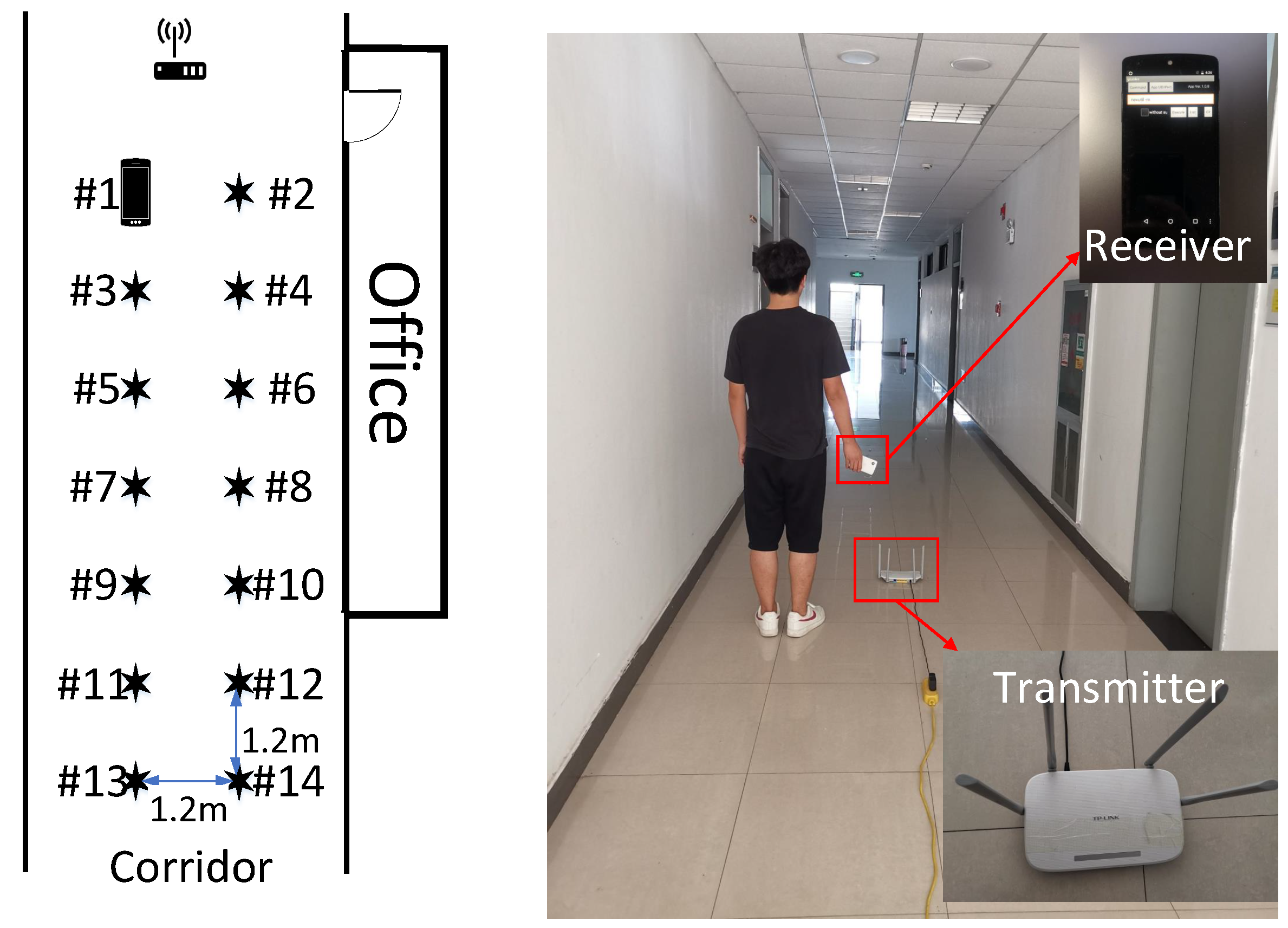
4.3. Experiment 3-Corridor
4.3.1. Setup
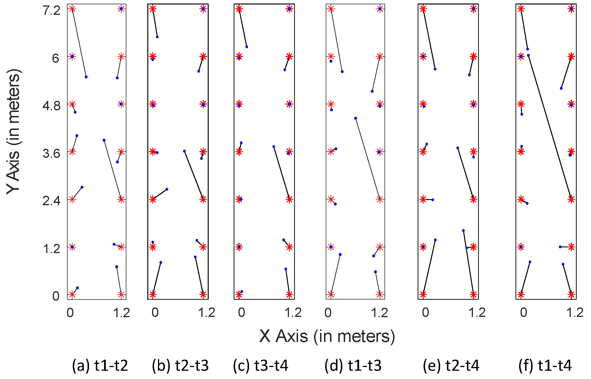
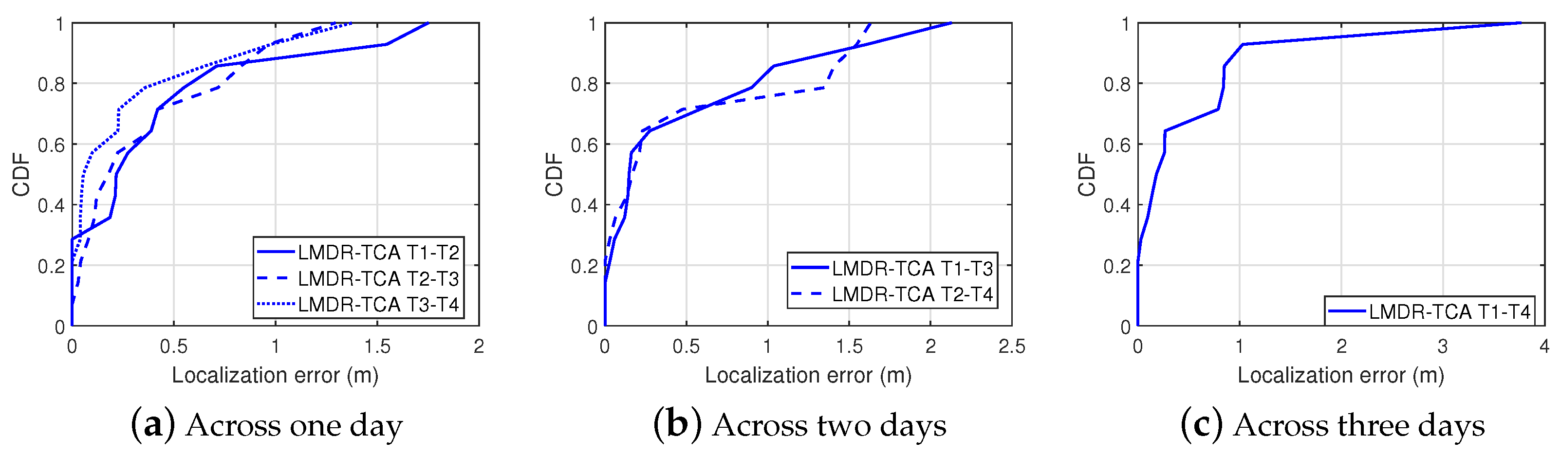
4.3.2. Localization Performance over Time
4.4. Analysis and Prospects
- (i)
- This paper proposes a novel indoor localization method for overcoming the problem of accuracy degradation because of time-varying Wi-Fi CSI readings. Experimental results verify that the proposed multi-domain representation mechanism plays a great role in improving localization accuracy, as with the fusion of the three alignment results after TCA, the max localization error decreases by up to 0.74 m compared to that obtained without using a combination of three representations.
- (ii)
- We chose TCA to shorten the distribution differences of two time-varying CSI readings, achieving approximately 48%, 78%, and 22% increases in classification performance, on average, compared with other traditional methods (KNN and SVM) and another transfer learning method (GFK).
- (iii)
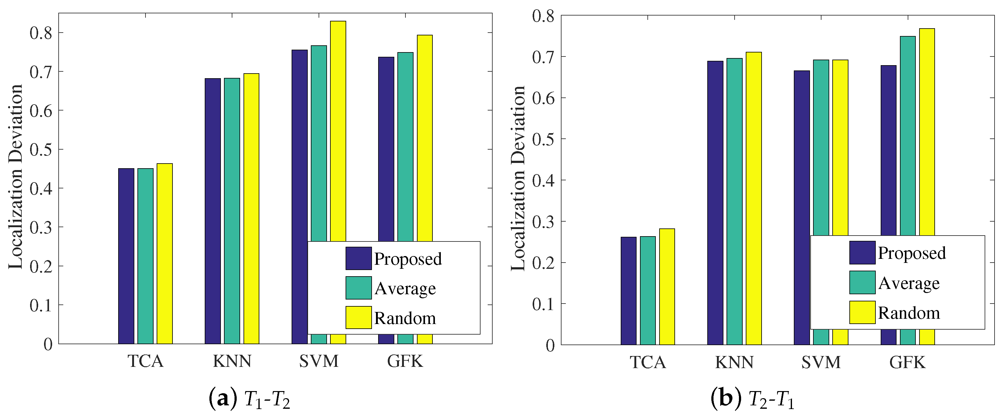
- We also evaluated the proposed novel fusion mechanism for position estimation using a combination of the Bayesian model averaging and weighted centroid algorithms. The correlation coefficients of the three representation models served as the weight, which outperformed the methods using random weights and average weights.
- (iv)
- In addition to a traditional computer platform based on an Intel Wi-Fi Link 5300 wireless network interface card, we also realized the experiments on a smartphone platform. Our method was proven effective even in an experiment that spanned three days.
- (v)
- Regarding the first and second experiments, we found an interesting phenomenon in which the experimental results of - were often better than those of -, whether in terms of the classification accuracy or positioning accuracy. The potential reason is the time difference in data collection. CSI values are influenced by many factors, such as multi-path effects, object obstacles, and even moving of targets upstairs or downstairs. These two groups of data may contain some noise affected by invisible factors, and we cannot tell which one is “cleaner”. We cannot ensure the relative stillness of an environment over time, and that is the reason that we explored a novel method for resolving this challenge in this paper. This interesting phenomenon may also inspire us to think about and research the impact of training data on the model performance and about how to judge the quality of training data.
- (vi)
- Another interesting experimental result was also found: In experiment 1, positions #13 and #5 were confused in all three representations, but in different ways. One reasonable explanation is that points #13 and #5 were on the same line in the geography, and the attenuation paths and multiple paths might have been similar. Inspired by this, we could explore the impact of the similarity of different areas/positions on fingerprinting localization in the work.
5. Conclusions
Author Contributions
Funding
Data Availability Statement
Conflicts of Interest
References
- Shu, Y.; Shin, K.G.; He, T.; Chen, J. Last-mile navigation using smartphones. In Proceedings of the ACM 21st Annual International Conference on Mobile Computing and Networking, Paris, France, 7–11 September 2015; pp. 512–524. [Google Scholar]
- Daud Kamal, M.; Tahir, A.; Babar Kamal, M.; Moeen, F.; Naeem, M.A. A Survey for the Ranking of Trajectory Prediction Algorithms on Ubiquitous Wireless Sensors. Sensors 2020, 20, 6495. [Google Scholar] [CrossRef] [PubMed]
- Wang, Y.; Tian, P.; Zhou, Y.; Chen, Q. The Encountered Problems and Solutions in the Development of Coal Mine Rescue Robot. J. Robot. 2018, 2018, 8471503. [Google Scholar] [CrossRef]
- Wang, Y.; Wu, K.; Ni, L.M. Wifall: Device-free fall detection by wireless networks. IEEE Trans. Mob. Comput. 2016, 16, 581–594. [Google Scholar] [CrossRef]
- Li, X.; Li, S.; Zhang, D.; Xiong, J.; Wang, Y.; Mei, H. Dynamic-music: Accurate device-free indoor localization. In Proceedings of the 2016 ACM International Joint Conference on Pervasive and Ubiquitous Computing, Heidelberg, Germany, 12–16 September 2016; pp. 196–207. [Google Scholar]
- Chang, L.; Xiong, J.; Wang, Y.; Chen, X.; Hu, J.; Fang, D. iUpdater: Low cost RSS fingerprints updating for device-free localization. In Proceedings of the 2017 IEEE 37th International Conference on Distributed Computing Systems (ICDCS), Atlanta, GA, USA, 5–8 June 2017; pp. 900–910. [Google Scholar]
- Guo, R.; Qin, D.; Zhao, M.; Wang, X. Indoor Radio Map Construction Based on Position Adjustment and Equipment Calibration. Sensors 2020, 20, 2818. [Google Scholar] [CrossRef]
- Kotaru, M.; Joshi, K.; Bharadia, D.; Katti, S. Spotfi: Decimeter level localization using wifi. In ACM SIGCOMM Computer Communication Review; ACM: New York, NY, USA, 2015; Volume 45, pp. 269–282. [Google Scholar]
- Seidel, S.Y.; Rappaport, T.S. 914 MHz path loss prediction models for indoor wireless communications in multifloored buildings. IEEE Trans. Antennas Propag. 1992, 40, 207–217. [Google Scholar] [CrossRef] [Green Version]
- Tian, Y.; Tang, Z.; Yu, Y. Third-order channel propagation model-based indoor adaptive localization algorithm for wireless sensor networks. IEEE Antennas Wirel. Propag. Lett. 2013, 12, 1578–1581. [Google Scholar] [CrossRef]
- Wu, K.; Xiao, J.; Yi, Y.; Gao, M.; Ni, L.M. Fila: Fine-grained indoor localization. In Proceedings of the IEEE INFOCOM, Orlando, FL, USA, 25–30 March 2012; pp. 2210–2218. [Google Scholar]
- Wang, X.; Gao, L.; Mao, S.; Pandey, S. CSI-based fingerprinting for indoor localization: A deep learning approach. IEEE Trans. Veh. Technol. 2016, 66, 763–776. [Google Scholar] [CrossRef] [Green Version]
- Wang, X.; Gao, L.; Mao, S. CSI phase fingerprinting for indoor localization with a deep learning approach. IEEE Internet Things J. 2016, 3, 1113–1123. [Google Scholar] [CrossRef]
- Wang, J.; Xiong, J.; Jiang, H.; Jamieson, K.; Chen, X.; Fang, D.; Wang, C. Low human-effort, device-free localization with fine-grained subcarrier information. IEEE Trans. Mob. Comput. 2018, 17, 2550–2563. [Google Scholar] [CrossRef]
- Abbas, M.; Elhamshary, M.; Rizk, H.; Torki, M.; Youssef, M. WiDeep: WiFi-based accurate and robust indoor localization system using deep learning. In Proceedings of the IEEE PerCom, Kyoto, Japan, 11–15 March 2019; Volume 19. [Google Scholar]
- Wang, B.; Liu, X.; Yu, B.; Jia, R.; Gan, X. An improved WiFi positioning method based on fingerprint clustering and signal weighted Euclidean distance. Sensors 2019, 19, 2300. [Google Scholar] [CrossRef] [Green Version]
- Liu, K.; Zhang, H.; Ng, J.K.Y.; Xia, Y.; Feng, L.; Lee, V.C.; Son, S.H. Toward low-overhead fingerprint-based indoor localization via transfer learning: Design, implementation, and evaluation. IEEE Trans. Ind. Inform. 2017, 14, 898–908. [Google Scholar] [CrossRef]
- Zou, H.; Zhou, Y.; Jiang, H.; Huang, B.; Xie, L.; Spanos, C. Adaptive localization in dynamic indoor environments by transfer kernel learning. In Proceedings of the 2017 IEEE Wireless Communications and Networking Conference (WCNC), San Francisco, CA, USA, 19–22 March 2017; pp. 1–6. [Google Scholar]
- Xiao, J.; Wu, K.; Yi, Y.; Wang, L.; Ni, L.M. Pilot: Passive device-free indoor localization using channel state information. In Proceedings of the 2013 IEEE 33rd International Conference on Distributed Computing Systems, Philadelphia, PA, USA, 8–11 July 2013; pp. 236–245. [Google Scholar]
- Yang, W.; Gong, L.; Man, D.; Lv, J.; Cai, H.; Zhou, X.; Yang, Z. Enhancing the performance of indoor device-free passive localization. Int. J. Distrib. Sens. Netw. 2015, 11, 256162. [Google Scholar] [CrossRef]
- Wang, J.; Gao, Q.; Cheng, P.; Yu, Y.; Xin, K.; Wang, H. Lightweight robust device-free localization in wireless networks. IEEE Trans. Ind. Electron. 2014, 61, 5681–5689. [Google Scholar] [CrossRef]
- Zhang, D.; Liu, Y.; Guo, X.; Ni, L.M. Rass: A real-time, accurate, and scalable system for tracking transceiver-free objects. IEEE Trans. Parallel Distrib. Syst. 2012, 24, 996–1008. [Google Scholar] [CrossRef]
- Youssef, M.; Mah, M.; Agrawala, A. Challenges: Device-free passive localization for wireless environments. In Proceedings of the 13th Annual ACM International Conference on Mobile Computing and Networking, Montreal, QC, Canada, 9–14 September 2007; pp. 222–229. [Google Scholar]
- Halperin, D.; Hu, W.; Sheth, A.; Wetherall, D. Predictable 802.11 packet delivery from wireless channel measurements. ACM SIGCOMM Comput. Commun. Rev. 2011, 41, 159–170. [Google Scholar]
- Yang, Z.; Zhou, Z.; Liu, Y. From RSSI to CSI: Indoor localization via channel response. ACM Comput. Surv. (CSUR) 2013, 46, 25. [Google Scholar] [CrossRef]
- Rai, A.; Chintalapudi, K.K.; Padmanabhan, V.N.; Sen, R. Zee: Zero-effort crowdsourcing for indoor localization. In Proceedings of the 18th ACM Annual International Conference on Mobile Computing and Networking, Istanbul, Turkey, 22–26 August 2012; pp. 293–304. [Google Scholar]
- Chen, H.; Zhang, Y.; Li, W.; Tao, X.; Zhang, P. ConFi: Convolutional neural networks based indoor Wi-Fi localization using channel state information. IEEE Access 2017, 5, 18066–18074. [Google Scholar] [CrossRef]
- Pan, S.J.; Tsang, I.W.; Kwok, J.T.; Yang, Q. Domain adaptation via transfer component analysis. IEEE Trans. Neural Netw. 2010, 22, 199–210. [Google Scholar] [CrossRef] [Green Version]
- Borgwardt, K.M.; Gretton, A.; Rasch, M.J.; Kriegel, H.P.; Schölkopf, B.; Smola, A.J. Integrating structured biological data by kernel maximum mean discrepancy. Bioinformatics 2006, 22, e49–e57. [Google Scholar] [CrossRef] [Green Version]
- Fragoso, T.M.; Bertoli, W.; Louzada, F. Bayesian model averaging: A systematic review and conceptual classification. Int. Stat. Rev. 2018, 86, 1–28. [Google Scholar] [CrossRef] [Green Version]
- Halperin, D.; Hu, W.; Sheth, A.; Wetherall, D. Tool release: Gathering 802.11 n traces with channel state information. ACM SIGCOMM Comput. Commun. Rev. 2011, 41, 53. [Google Scholar] [CrossRef]
- Gong, B.; Shi, Y.; Sha, F.; Grauman, K. Geodesic flow kernel for unsupervised domain adaptation. In Proceedings of the 2012 IEEE Conference on Computer Vision and Pattern Recognition, Providence, RI, USA, 16–21 June 2012; pp. 2066–2073. [Google Scholar]
- Schulz, M.; Link, J.; Gringoli, F.; Hollick, M. Shadow Wi-Fi: Teaching Smartphones to Transmit Raw Signals and to Extract Channel State Information to Implement Practical Covert Channels over Wi-Fi. In Proceedings of the ACM 16th Annual International Conference on Mobile Systems, Applications, and Services, Munich, Germany, 10–15 June 2018; pp. 256–268. [Google Scholar]


| - | - | |||||||
|---|---|---|---|---|---|---|---|---|
| LMDR- | TCA | KNN | SVM | GFK | TCA | KNN | SVM | GFK |
| Mean deviation | 0.2227 | 0.3301 | 0.398 | 0.2737 | 0.0678 | 0.4335 | 0.3596 | 0.2362 |
| Max deviation | 1.6558 | 1.9187 | 1.911 | 1.9733 | 1.0525 | 2.5903 | 2.4034 | 1.6081 |
| - | - | |||||||
|---|---|---|---|---|---|---|---|---|
| LMDR- | TCA | KNN | SVM | GFK | TCA | KNN | SVM | GFK |
| Mean deviation | 0.4547 | 0.6814 | 0.7547 | 0.7367 | 0.2611 | 0.6887 | 0.6653 | 0.6783 |
| Max deviation | 2.7514 | 3.761 | 4.3716 | 5.0876 | 4.0353 | 4.3267 | 4.3267 | 4.3267 |
| Interval Days | One Day | Two Days | Three Days | |||
|---|---|---|---|---|---|---|
| Source-Target | - | - | - | - | - | - |
| Mean error (m) | 0.4466 | 0.3855 | 0.2926 | 0.5132 | 0.5174 | 0.5888 |
| Max error (m) | 1.7514 | 1.2945 | 1.3788 | 2.1294 | 1.6323 | 3.7698 |
Publisher’s Note: MDPI stays neutral with regard to jurisdictional claims in published maps and institutional affiliations. |
© 2021 by the authors. Licensee MDPI, Basel, Switzerland. This article is an open access article distributed under the terms and conditions of the Creative Commons Attribution (CC BY) license (http://creativecommons.org/licenses/by/4.0/).
Share and Cite
Yin, Y.; Yang, X.; Li, P.; Zhang, K.; Chen, P.; Niu, Q. Localization with Transfer Learning Based on Fine-Grained Subcarrier Information for Dynamic Indoor Environments. Sensors 2021, 21, 1015. https://0-doi-org.brum.beds.ac.uk/10.3390/s21031015
Yin Y, Yang X, Li P, Zhang K, Chen P, Niu Q. Localization with Transfer Learning Based on Fine-Grained Subcarrier Information for Dynamic Indoor Environments. Sensors. 2021; 21(3):1015. https://0-doi-org.brum.beds.ac.uk/10.3390/s21031015
Chicago/Turabian StyleYin, Yuqing, Xu Yang, Peihao Li, Kaiwen Zhang, Pengpeng Chen, and Qiang Niu. 2021. "Localization with Transfer Learning Based on Fine-Grained Subcarrier Information for Dynamic Indoor Environments" Sensors 21, no. 3: 1015. https://0-doi-org.brum.beds.ac.uk/10.3390/s21031015