
Automatic Ankle Angle Detection by Integrated RGB and Depth Camera System

 , and
, and
Abstract
:1. Introduction
2. Related Work
3. Materials and Methods
3.1. Tests
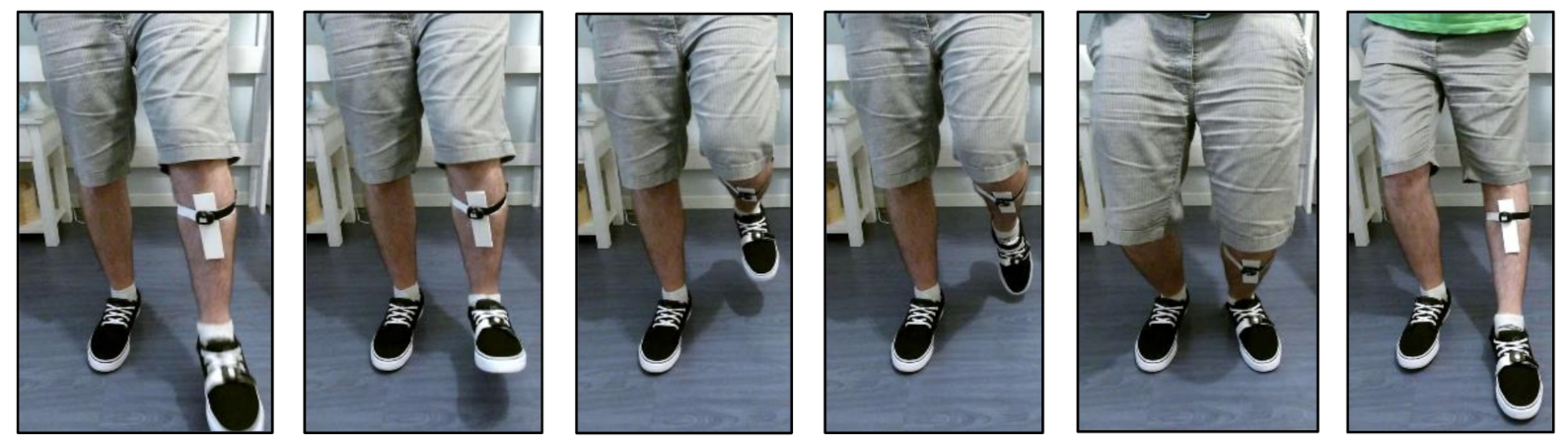
3.1.1. Fixed Distance Tests
3.1.2. Walking Test
3.2. Experimental Setup
3.2.1. Kinect v2-Integrated RGB and Depth Camera System
3.2.2. Inertial Measurement Units for Angle Detection
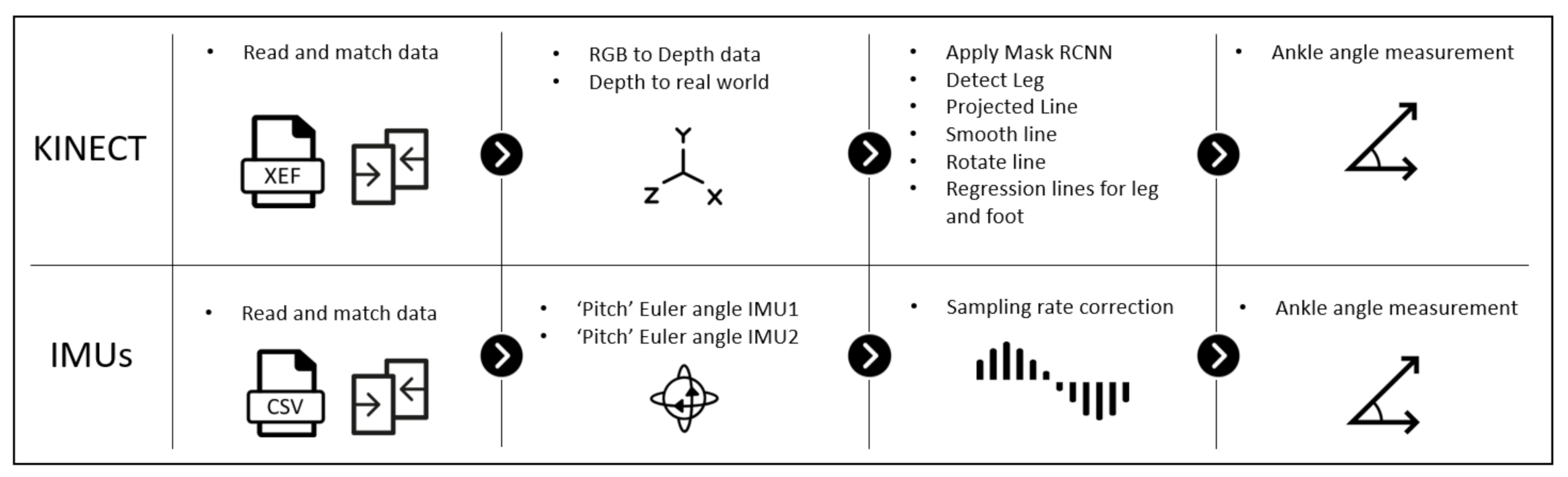
3.3. Methods
3.3.1. Data Acquisition
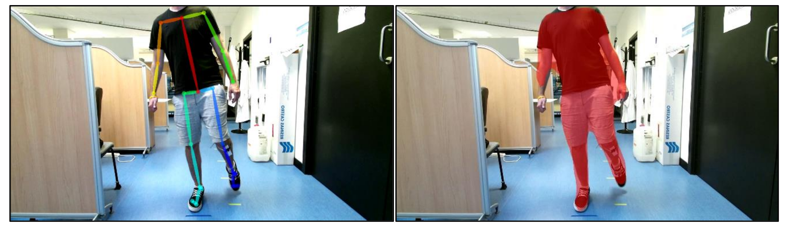
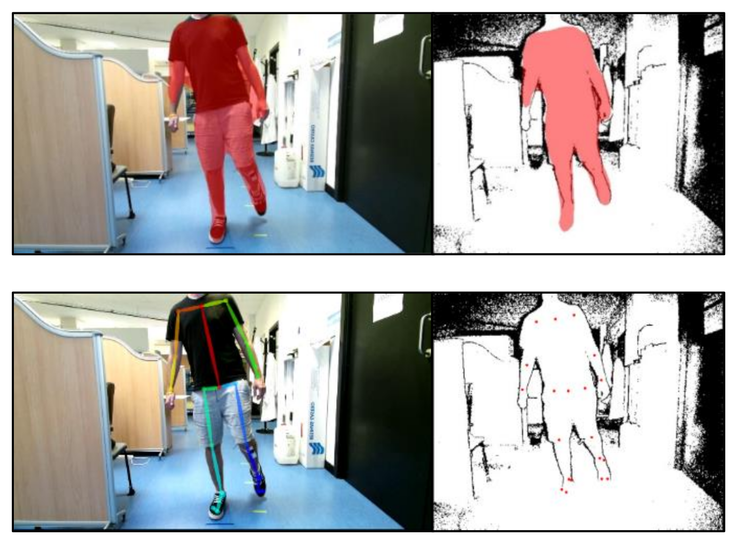
3.3.2. Body Recognition for RGB and Depth Images
3.3.3. Ankle Angle Measurement
3.3.4. Statistics
3.3.5. Propagation of Uncertainty
4. Results
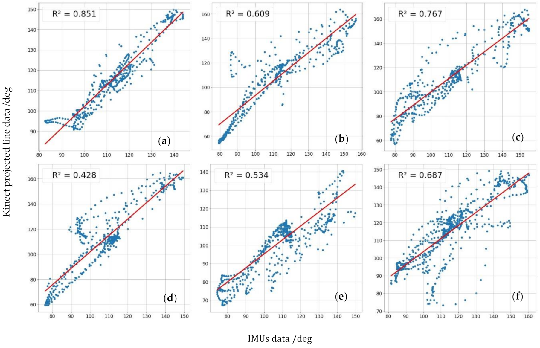
4.1. Distance Tests
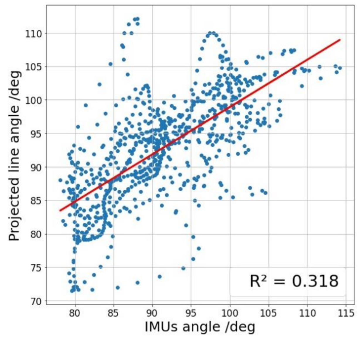
4.2. Walking Test
5. Discussion
6. Conclusions
Author Contributions
Funding
Informed Consent Statement
Data Availability Statement
Conflicts of Interest
References
- Tinetti, M.E.; Speechley, M.; Ginter, S.F. Risk Factors for Falls among Elderly Persons Living in the Community. N. Engl. J. Med. 1988, 319, 1701–1707. [Google Scholar] [CrossRef]
- Tinetti, M.E.; De Leon, C.F.M.; Doucette, J.T.; Baker, D.I. Fear of Falling and Fall-Related Efficacy in Relationship to Functioning Among Community-Living Elders. J. Gerontol. 1994, 49, M140–M147. [Google Scholar] [CrossRef]
- Baker, R. Gait analysis methods in rehabilitation. J. Neuroeng. Rehabil. 2006, 3, 4. [Google Scholar] [CrossRef] [Green Version]
- Gouwanda, D.; Senanayake, S.M.N.A. Emerging Trends of Body-Mounted Sensors in Sports and Human Gait Analysis. In Proceedings of the 4th Kuala Lumpur International Conference on Biomedical Engineering, Kuala Lumpur, Malaysia, 25–28 June 2008. [Google Scholar]
- Gard, S.A. Use of Quantitative Gait Analysis for the Evaluation of Prosthetic Walking Performance. JPO J. Prosthetics Orthot. 2006, 18, P93–P104. [Google Scholar] [CrossRef]
- Hao, S.; Dawei, W.; Rongjie, K.; Yan, C. Gait analysis and control of a deployable robot. Mech. Mach. Theory 2018, 120, 107–119. [Google Scholar]
- Bridenbaugh, S.A.; Kressig, R.W. Laboratory Review: The Role of Gait Analysis in Seniors’ Mobility and Fall Prevention. Gerontology 2010, 57, 256–264. [Google Scholar] [CrossRef] [Green Version]
- Woollacott, M.; Shumway-Cook, A. Attention and the control of posture and gait: A review of an emerging area of research. Gait Posture 2002, 16, 1–14. [Google Scholar] [CrossRef]
- Dubois, A.; Bihl, T.; Bresciani, J.-P. Automating the Timed Up and Go Test Using a Depth Camera. Sensors 2017, 18, 14. [Google Scholar] [CrossRef] [Green Version]
- Steinert, A.; Sattler, I.; Otte, K.; Röhling, H.; Mansow-Model, S.; Müller-Werdan, U. Using New Camera-Based Technologies for Gait Analysis in Older Adults in Comparison to the Established GAITRite System. Sensors 2019, 20, 125. [Google Scholar] [CrossRef] [Green Version]
- Capecci, M.; Ceravolo, M.G.; Ferracuti, F.; Iarlori, S.; Longhi, S.; Romeo, L.; Russi, S.N.; Verdini, F. Accuracy evaluation of the Kinect v2 sensor during dynamic movements in a rehabilitation scenario. In Proceedings of the 2016 38th Annual International Conference of the IEEE Engineering in Medicine and Biology Society (EMBC), Orlando, FL, USA, 6 August 2016; Volume 2016, pp. 5409–5412. [Google Scholar]
- Paolini, G.; Peruzzi, A.; Mirelman, A.; Cereatti, A.; Gaukrodger, S.; Hausdorff, J.M.; Della Croce, U. Validation of a Method for Real Time Foot Position and Orientation Tracking With Microsoft Kinect Technology for Use in Virtual Reality and Treadmill Based Gait Training Programs. IEEE Trans. Neural Syst. Rehabil. Eng. 2013, 22, 997–1002. [Google Scholar] [CrossRef]
- Tan, D.; Pua, Y.-H.; Balakrishnan, S.; Scully, A.; Bower, K.J.; Prakash, K.M.; Tan, E.-K.; Chew, J.-S.; Poh, E.; Tan, S.-B.; et al. Automated analysis of gait and modified timed up and go using the Microsoft Kinect in people with Parkinson’s disease: Associations with physical outcome measures. Med. Biol. Eng. Comput. 2018, 57, 369–377. [Google Scholar] [CrossRef]
- Liu, L.; Mehrotra, S. Patient walk detection in hospital room using Microsoft Kinect V2. In Proceedings of the 2016 38th Annual International Conference of the IEEE Engineering in Medicine and Biology Society (EMBC), Orlando, FL, USA, 16–20 August 2016; pp. 4395–4398. [Google Scholar]
- Cippitelli, E.; Gasparrini, S.; Spinsante, S.; Gambi, E. Kinect as a Tool for Gait Analysis: Validation of a Real-Time Joint Extraction AlgorithmWorking in Side View. Sensors 2015, 15, 1417–1434. [Google Scholar]
- Geerse, D.; Coolen, B.; Kolijn, D.; Roerdink, M. Validation of Foot Placement Locations from Ankle Data of a Kinect v2 Sensor. Sensors 2017, 17, 2301. [Google Scholar] [CrossRef] [Green Version]
- Lin, P.-Y.; Yang, Y.-R.; Cheng, S.-J.; Wang, R.-Y. The Relation Between Ankle Impairments and Gait Velocity and Symmetry in People With Stroke. Arch. Phys. Med. Rehabil. 2006, 87, 562–568. [Google Scholar] [CrossRef]
- Buck, P.; Morrey, B.F.; Chao, E.Y. The optimum position of arthrodesis of the ankle. A gait study of the knee and ankle. J. Bone Jt. Surg. Am. 1987, 69, 1052–1062. [Google Scholar]
- Seel, T.; Raisch, J.; Schauer, T. IMU-Based Joint Angle Measurement for Gait Analysis. Sensors 2014, 14, 6891–6909. [Google Scholar] [CrossRef] [Green Version]
- Otte, K.; Kayser, B.; Mansow-Model, S.; Verrel, J.; Paul, F.; Brandt, A.U.; Schmitz-Hübsch, T. Accuracy and Reliability of the Kinect Version 2 for Clinical Measurement of Motor Function. PLoS ONE 2016, 11, e0166532. [Google Scholar] [CrossRef]
- Cao, Z.; Hidalgo Martinez, G.; Simon, T.; Wei, S.-E.; Sheikh, Y.A. OpenPose: Realtime Multi-Person 2D Pose Estimation using Part Affinity Fields. IEEE Trans. Pattern Anal. Mach. Intell. 2019, 1–14, in press. [Google Scholar] [CrossRef] [Green Version]
- Kharazi, M.R.; Memari, A.H.; Shahrokhi, A.; Nabavi, H.; Khorami, S.; Rasooli, A.H.; Barnamei, H.R.; Jamshidian, A.R.; Mirbagheri, M.M. Validity of Microsoft KinectTM for measuring gait parameters. In Proceedings of the 22nd Iranian Conference on Biomedical Engineering(ICBME 2015), Iranian Research Organization for Science and Technology (IROST), Tehran, Iran, 25–27 November 2015. [Google Scholar]
- Jamali, Z.; Behzadipour, S. Quantitative evaluation of parameters affecting the accuracy of Microsoft Kinect in GAIT analysis. In Proceedings of the 2016 23rd Iranian Conference on Biomedical Engineering and 2016 1st International Iranian Conference on Biomedical Engineering (ICBME), Tehran, Iran, 24–25 November 2016; IEEE: New York, NY, USA, 2016; pp. 306–311. [Google Scholar]
- Wang, Q.; Kurillo, G.; Ofli, F.; Bajcsy, R. Evaluation of Pose Tracking Accuracy in the First and Second Generations of Microsoft Kinect. In Proceedings of the 2015 International Conference on Healthcare Informatics, Dallas, TX, USA, 21–23 October 2015; pp. 380–389. [Google Scholar]
- Eltoukhy, M.; Oh, J.; Kuenze, C.; Signorile, J. Improved kinect-based spatiotemporal and kinematic treadmill gait assessment. Gait Posture 2017, 51, 77–83. [Google Scholar] [CrossRef]
- Lamine, H.; Bennour, S.; Laribi, M.; Romdhane, L.; Zaghloul, S. Evaluation of Calibrated Kinect Gait Kinematics Using a Vicon Motion Capture System. Comput. Methods Biomech. Biomed. Eng. 2017, 20, S111–S112. [Google Scholar] [CrossRef] [Green Version]
- Oh, J.; Kuenze, C.; Jacopetti, M.; Signorile, J.F.; Eltoukhy, M. Validity of the Microsoft Kinect™ in assessing spatiotemporal and lower extremity kinematics during stair ascent and descent in healthy young individuals. Med. Eng. Phys. 2018, 60, 70–76. [Google Scholar] [CrossRef]
- Bilesan, A.; Owlia, M.; Behzadipour, S.; Ogawa, S.; Tsujita, T.; Komizunai, S.; Konno, A. Marker-based motion tracking using Microsoft Kinect. IFAC-PapersOnLine 2018, 51, 399–404. [Google Scholar] [CrossRef]
- Latorre, J.; Colomer, C.; Alcañiz, M.; Llorens, R. Gait analysis with the Kinect v2: Normative study with healthy individuals and comprehensive study of its sensitivity, validity, and reliability in individuals with stroke. J. Neuroeng. Rehabil. 2019, 16, 1–11. [Google Scholar]
- D’ Eusanio, A.; Pini, S.; Borghi, G.; Vezzani, R.; Cucchiara, R. Manual Annotations on Depth Maps for Human Pose Estimation. In Mathematics and Computation in Music; Springer Science and Business Media LLC: Berlin/Heidelberg, Germany, 2019; pp. 233–244. [Google Scholar]
- Shotton, J.; Sharp, T.; Kipman, A.; FitzGibbon, A.; Finocchio, M.; Blake, A.; Cook, M.; Moore, R. Real-time human pose recognition in parts from single depth images. Commun. ACM 2013, 56, 116–124. [Google Scholar] [CrossRef] [Green Version]
- Haque, A.; Peng, B.; Luo, Z.; Alahi, A.; Yeung, S.; Fei-Fei, L. Towards Viewpoint Invariant 3D Human Pose Estimation. In Machine Learning and Knowledge Discovery in Databases, Proceedings of the Applied Data Science and Demo Track, Amsterdam, The Netherlands, 11–14 October 2016; Springer Science and Business Media LLC: Berlin/Heidelberg, Germany, 2016; pp. 160–177. [Google Scholar]
- Ballotta, D.; Borghi, G.; Vezzani, R.; Cucchiara, R. Fully Convolutional Network for Head Detection with Depth Images. In Proceedings of the 2018 24th International Conference on Pattern Recognition (ICPR), Beijing, China, 20–24 August 2018; pp. 752–757. [Google Scholar]
- D’Antonio, E.; Taborri, J.; Palermo, E.; Rossi, S.; Patane, F. A markerless system for gait analysis based on OpenPose library. In Proceedings of the 2020 IEEE International Instrumentation and Measurement Technology Conference (I2MTC), Dubrovnik, Croatia, 25–28 May 2020; pp. 1–6. [Google Scholar] [CrossRef]
- Stenum, J.; Rossi, C.; Roemmich, R. Two-dimensional video-based analysis of human gait using pose estimation. Biorxiv 2020. [Google Scholar]
- Lee, D.-S.; Kim, J.-S.; Jeong, S.C.; Kwon, S.-K. Human Height Estimation by Color Deep Learning and Depth 3D Conversion. Appl. Sci. 2020, 10, 5531. [Google Scholar] [CrossRef]
- Junkins, J.L.; Shuster, M.D. The Geometry of the Euler Angles. J. Astronaut. Sci. 1993, 41, 531–543. [Google Scholar]
- Pagliari, D.; Pinto, L. Calibration of Kinect for Xbox One and Comparison between the Two Generations of Microsoft Sensors. Sensors 2015, 15, 27569–27589. [Google Scholar] [CrossRef] [Green Version]
- He, K.; Gkioxari, G.; Dollár, P.; Girshick, R. Mask R-CNN. arXiv 2018. [Google Scholar]
- Mask R-CNN for Object Detection and Instance Segmentation on Keras and TensorFlow. 2018. Available online: https://github.com/matterport/Mask_RCNN. (accessed on 4 April 2020).
- Hidalgo, G.; Cao, Z.; Simon, T.; Wei, S.-E.; Raaj, Y.; Joo, H.; Sheikh, Y. Available online: https://github.com/CMU-Perceptual-Computing-Lab/openpose (accessed on 22 October 2020).


| Distance/m | f |
|---|---|
| 0.5 | 0.65 |
| 1 | 0.65 |
| 1.5 | 0.75 |
| 2 | 0.8 |
| 3 | 0.9 |
| 4 | 0.95 |
| Pearson, r [95%CI] | [95%CI] | |||||
|---|---|---|---|---|---|---|
| Distance/m | Projected Line | OpenPose | Default Skeleton | Projected Line | OpenPose | Default Skeleton |
| 0.5 | 0.95 (0.94, 0.96) | - | - | 0.94 (0.93, 0.95) | - | - |
| 1 | 0.90 (0.88, 0.91) | 0.60 (0.55, 0.66) | 0.86 (0.84, 0.88) | 0.90 (0.88, 0.91) | 0.60 (0.54, 0.65) | 0.89 (0.87, 0.90) |
| 1.5 | 0.92 (0.90, 0.93) | 0.61 (0.55, 0.67) | 0.19 (0.10, 0.28) | 0.91 (0.89, 0.92) | 0.66 (0.60, 0.71) | 0.33 (0.25, 0.41) |
| 2 | 0.89 (0.87, 0.91) | 0.74 (0.70, 0.77) | 0.33 (0.25, 0.41) | 0.75 (0.71, 0.78) | 0.75 (0.71, 0.78) | 0.50 (0.43, 0.56) |
| 3 | 0.85 (0.83, 0.87) | 0.28 (0.22, 0.35) | 0.74 (0.70, 0.77) | 0.67 (0.63, 0.71) | 0.18 (0.11, 0.25) | 0.57 (0.51, 0.61) |
| 4 | 0.83 (0.80, 0.85) | 0.43 (0.37, 0.49) | 0.28 (0.21, 0.35) | 0.85 (0.83, 0.87) | 0.25 (0.18, 0.32) | 0.38 (0.31, 0.44) |
| Mean ± SD | 0.89 ± 0.04 | 0.53 ± 0.15 | 0.4 ± 0.2 | 0.83 ± 0.09 | 0.5 ± 0.2 | 0.5 ± 0.2 |
| RMSE/deg | MAE/deg | |||||
|---|---|---|---|---|---|---|
| Distance/m | Projected Line | OpenPose | Default Skeleton | Projected Line | OpenPose | Default Skeleton |
| 0.5 | 5.50 | - | - | 4.40 | - | - |
| 1 | 13.40 | 19.10 | 12.20 | 9.90 | 11.71 | 8.22 |
| 1.5 | 10.50 | 24.20 | 28.80 | 7.70 | 16.90 | 17.40 |
| 2 | 13.60 | 16.50 | 19.10 | 10.00 | 10.72 | 11.30 |
| 3 | 10.69 | 23.40 | 14.90 | 7.49 | 14.53 | 9.70 |
| 4 | 10.60 | 18.37 | 30.70 | 7.40 | 14.50 | 21.00 |
| Mean ± SD | 10 ± 2 | 20 ± 3 | 20 ± 4 | 7.5 ± 1.8 | 13 ± 2 | 13 ± 7. |
| Pearson, r (95% CI) | [95%CI] | ||||
|---|---|---|---|---|---|
| Projected Line | OpenPose | Default Skeleton | Projected Line | OpenPose | Default Skeleton |
| 0.74 (0.78,0.70) | 0.25 (0.20, 0.30) | - | 0.72 (0.68, 0.74) | 0.26 (0.20, 0.32) | - |
| RMSE/deg | MAE/deg | ||||
|---|---|---|---|---|---|
| Projected Line | OpenPose | Default Skeleton | Projected Line | OpenPose | Default Skeleton |
| 6.39 | 11.75 | - | 4.76 | 8.63 | - |
Publisher’s Note: MDPI stays neutral with regard to jurisdictional claims in published maps and institutional affiliations. |
© 2021 by the authors. Licensee MDPI, Basel, Switzerland. This article is an open access article distributed under the terms and conditions of the Creative Commons Attribution (CC BY) license (http://creativecommons.org/licenses/by/4.0/).
Share and Cite
Díaz-San Martín, G.; Reyes-González, L.; Sainz-Ruiz, S.; Rodríguez-Cobo, L.; López-Higuera, J.M. Automatic Ankle Angle Detection by Integrated RGB and Depth Camera System. Sensors 2021, 21, 1909. https://0-doi-org.brum.beds.ac.uk/10.3390/s21051909
Díaz-San Martín G, Reyes-González L, Sainz-Ruiz S, Rodríguez-Cobo L, López-Higuera JM. Automatic Ankle Angle Detection by Integrated RGB and Depth Camera System. Sensors. 2021; 21(5):1909. https://0-doi-org.brum.beds.ac.uk/10.3390/s21051909
Chicago/Turabian StyleDíaz-San Martín, Guillermo, Luis Reyes-González, Sergio Sainz-Ruiz, Luis Rodríguez-Cobo, and José M. López-Higuera. 2021. "Automatic Ankle Angle Detection by Integrated RGB and Depth Camera System" Sensors 21, no. 5: 1909. https://0-doi-org.brum.beds.ac.uk/10.3390/s21051909