
Imbalanced Loss-Integrated Deep-Learning-Based Ultrasound Image Analysis for Diagnosis of Rotator-Cuff Tear


Abstract
:1. Introduction
2. Methods
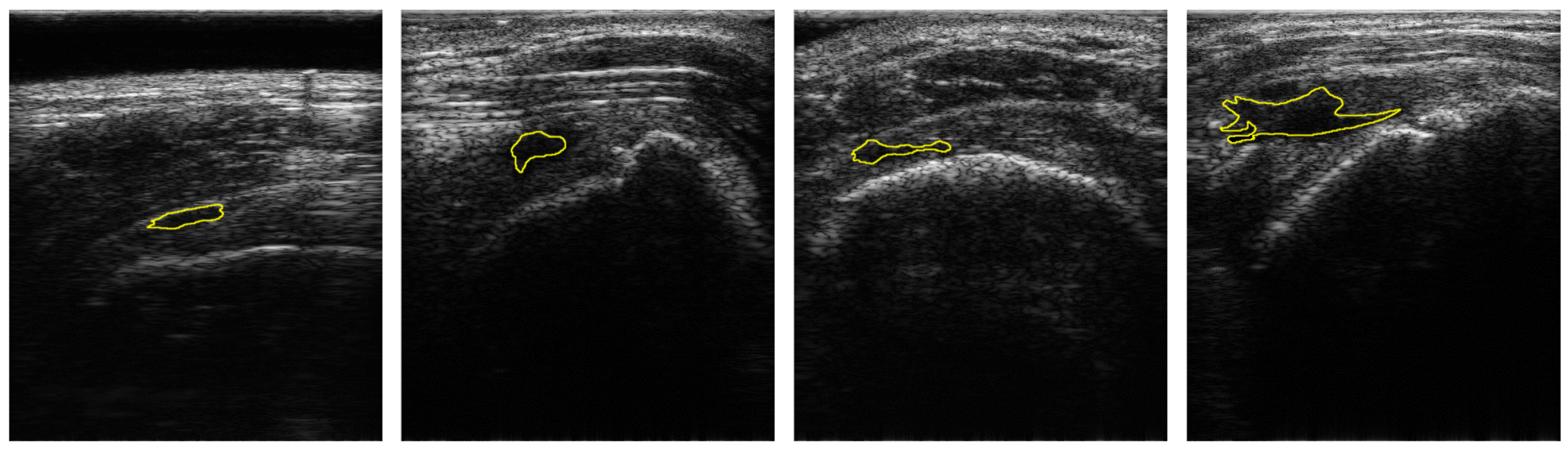
2.1. Dataset
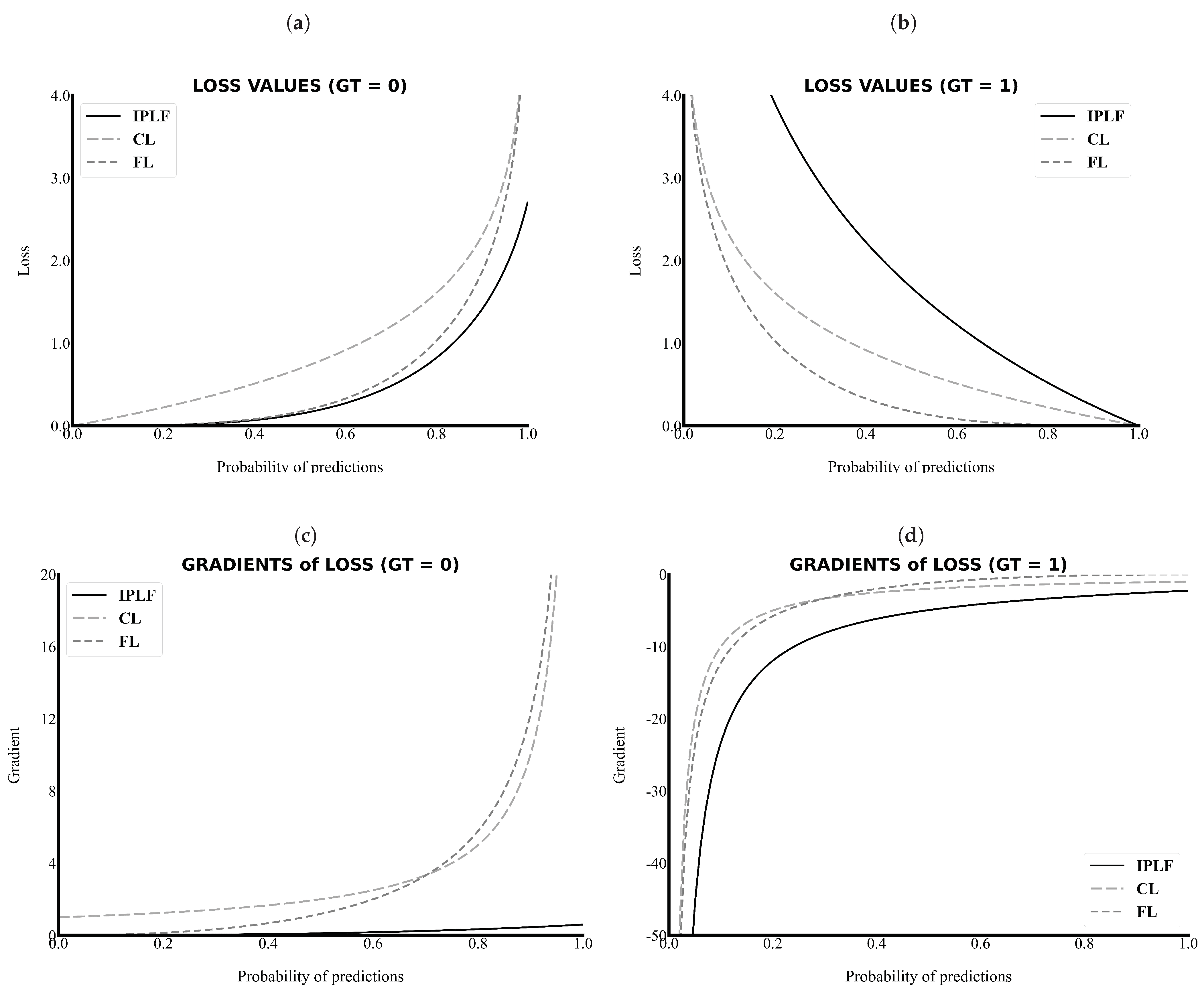
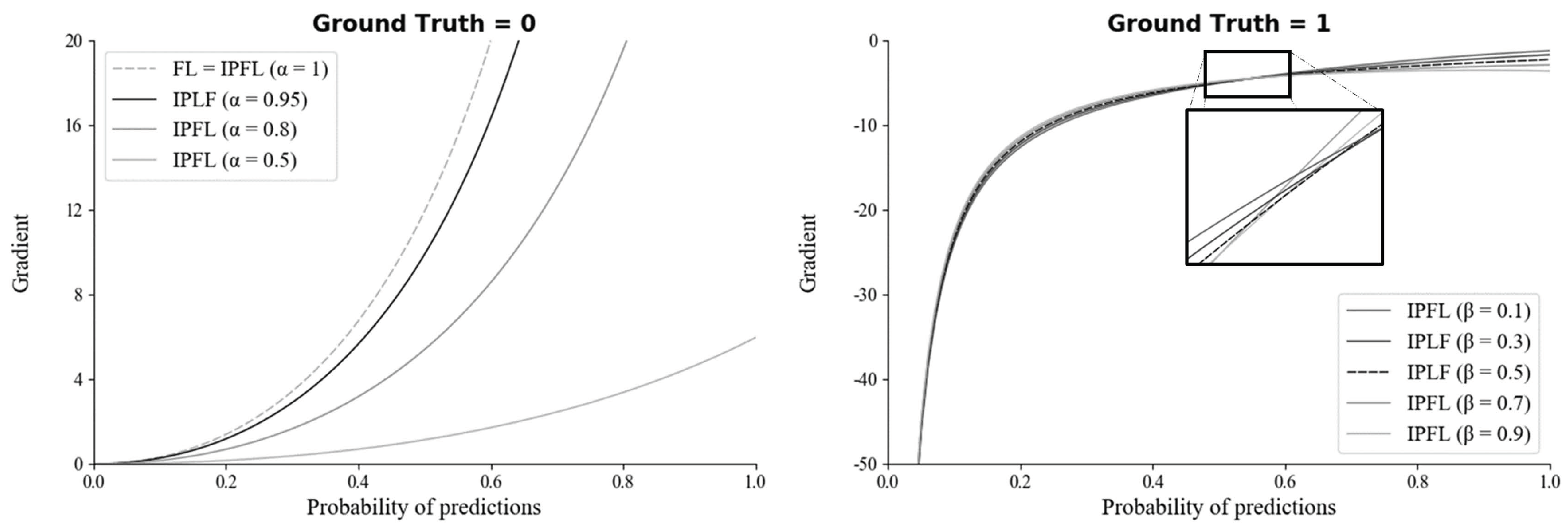
2.2. Integrated-on-Positive-Loss Function
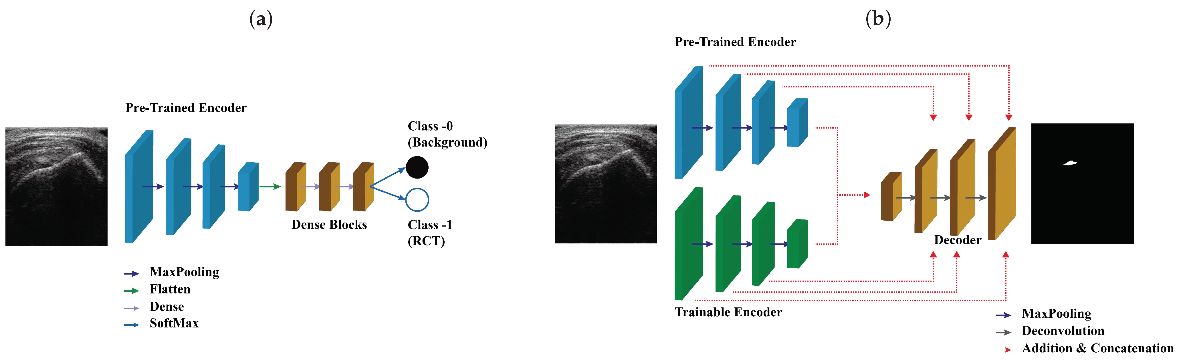
2.3. Architecture of the SMART-CA
2.4. Training of SMART-CA
2.5. Experimental Setup
2.6. Evaluation Metrics
3. Results
3.1. Effects of IPLF in the Segmentation of RCT
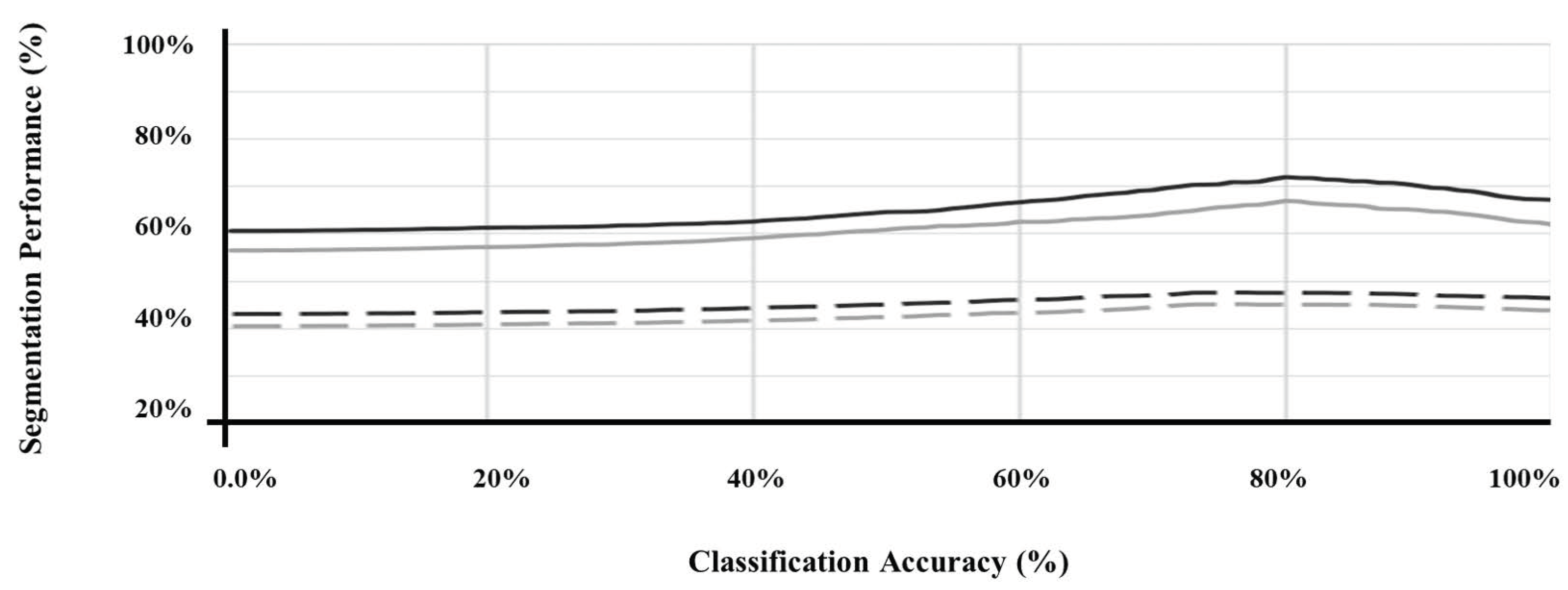
3.2. Evaluation of Performance of SMART-CA for the Segmentation of RCT in US Images
4. Discussion
4.1. Analysis of SMART-CA
4.2. Analysis of IPLF
4.3. Feature Extraction by SMART-CA
4.4. Analysis of Results
5. Conclusions
Author Contributions
Funding
Institutional Review Board Statement
Informed Consent Statement
Data Availability Statement
Conflicts of Interest
Appendix A
Appendix A.1.

| Name | Image Size | Operation | Channel | |
|---|---|---|---|---|
| Input image | 3 | |||
| Part I | Down 1 | Conv | 64 | |
| Conv | 64 | |||
| Maxpooling (SeLU) | 64 | |||
| Down 2 | Conv | 128 | ||
| Conv | 128 | |||
| Maxpooling (SeLU) | 128 | |||
| Down 3 | Conv | 256 | ||
| Conv | 256 | |||
| Conv | 256 | |||
| Conv | 256 | |||
| Maxpooling (SeLU) | 256 | |||
| Down 4 | Conv | 512 | ||
| Conv | 512 | |||
| Conv | 512 | |||
| Conv | 512 | |||
| Maxpooling (SeLU) | 512 | |||
| Part II | Flatten | 1 | Flatten | |
| Fully Connected 1 | 1 | Dense (SeLU activation) | 4096 | |
| Fully Connected 2 | 1 | Dense (SeLU activation) | 4096 | |
| Fully Connected 3 | 1 | Dense (None activation) | 2 | |
| SoftMax | 1 | SoftMax | 2 |
| Name | Image Size | Operation | Channel | ||
|---|---|---|---|---|---|
| Pre-Trained Encoder | Trainable Encoder | ||||
| Input image | 3 | ||||
| Encoder | Down 1 | Conv | Conv | 64 | |
| Conv | Conv | 64 | |||
| Maxpooling (SeLU) | 64 | ||||
| Down 2 | Conv | Conv | 128 | ||
| Conv | Conv | 128 | |||
| Maxpooling (SeLU) | 128 | ||||
| Down 3 | Conv | Conv | 256 | ||
| Conv | Conv | 256 | |||
| Conv | Conv | 256 | |||
| Conv | Conv | 256 | |||
| Maxpooling (SeLU) | 256 | ||||
| Down 4 | Conv | Conv | 512 | ||
| Conv | Conv | 512 | |||
| Conv | Conv | 512 | |||
| Conv | Conv | 512 | |||
| Maxpooling (SeLU) | 512 | ||||
| Bridge | Bottom | Addition (Down 4) | 512 | ||
| Conv | 512 | ||||
| Conv | 512 | ||||
| Decoder | Upsampling 1 | Deconv(Bottom) + Conv | 512 | ||
| Concatenate(Upsampling1, Down 4) | 1024 | ||||
| Conv | 512 | ||||
| Conv | 512 | ||||
| Upsampling 2 | Deconv(Upsampling1) + Conv | 256 | |||
| Concatenate(Upsampling2, Down 3) | 512 | ||||
| Conv | 256 | ||||
| Conv | 256 | ||||
| Upsampling 3 | Deconv(Upsampling2) + Conv | 128 | |||
| Concatenate(Upsampling3, Down 2) | 256 | ||||
| Conv | 128 | ||||
| Conv | 128 | ||||
| Upsampling 4 | Deconv(Upsampling4) + Conv | 64 | |||
| Concatenate(Upsampling3, Down 1) | 128 | ||||
| Conv | 64 | ||||
| Conv | 64 | ||||
| Logit | Logit | Conv | 64 | ||
| Conv | 2 | ||||
| SoftMax | 2 | ||||
Appendix A.2.
Appendix B
Appendix B.1.
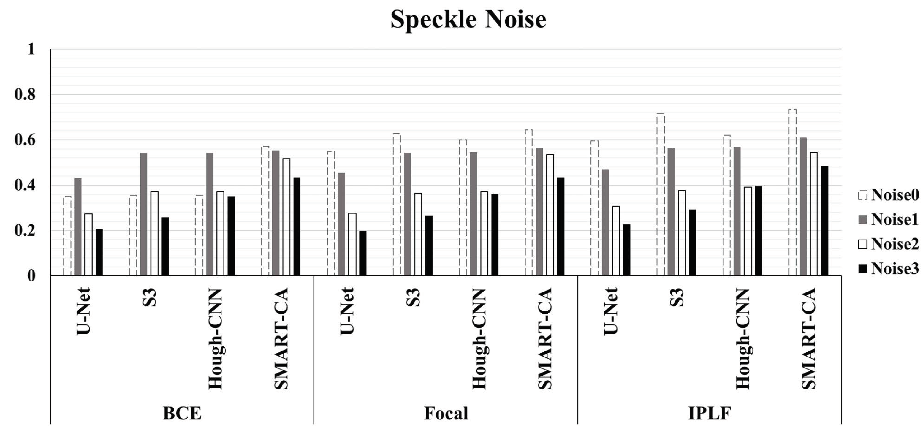
| Speckle | Metric | U-Net | Hough-CNN | SMART-CA | |||||||||
|---|---|---|---|---|---|---|---|---|---|---|---|---|---|
| BCE | Focal | IPLF | BCE | Focal | IPLF | BCE | Focal | IPLF | BCE | Focal | IPLF | ||
| Original | Precision | 0.22 | 0.406 | 0.459 | 0.222 | 0.512 | 0.665 | 0.224 | 0.475 | 0.476 | 0.443 | 0.518 | 0.604 |
| Recall | 0.85 | 0.845 | 0.846 | 0.885 | 0.815 | 0.772 | 0.842 | 0.816 | 0.894 | 0.802 | 0.853 | 0.942 | |
| D.C. | 0.35 | 0.549 | 0.595 | 0.355 | 0.629 | 0.715 | 0.354 | 0.6 | 0.621 | 0.571 | 0.645 | 0.736 | |
| Accuracy | 0.655 | 0.848 | 0.874 | 0.649 | 0.895 | 0.933 | 0.664 | 0.881 | 0.881 | 0.868 | 0.897 | 0.926 | |
| B.A. | 0.740 | 0.847 | 0.862 | 0.752 | 0.860 | 0.862 | 0.742 | 0.853 | 0.887 | 0.839 | 0.878 | 0.933 | |
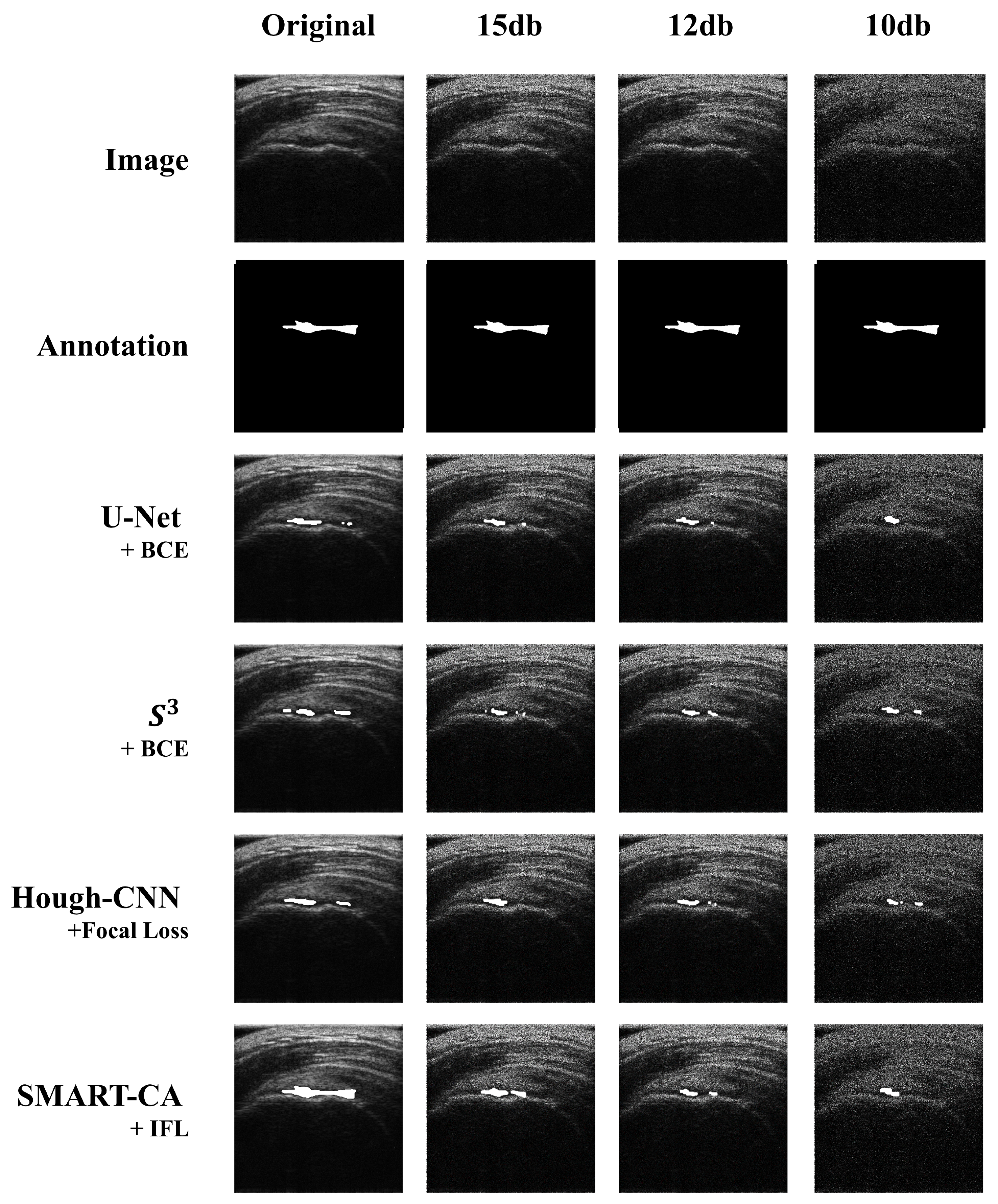
| PSNR = 15 | Precision | 0.296 | 0.316 | 0.322 | 0.423 | 0.414 | 0.437 | 0.413 | 0.411 | 0.478 | 0.42 | 0.425 | 0.426 |
| Recall | 0.795 | 0.806 | 0.869 | 0.755 | 0.793 | 0.793 | 0.794 | 0.805 | 0.839 | 0.81 | 0.85 | 0.857 | |
| D.C. | 0.431 | 0.454 | 0.47 | 0.543 | 0.544 | 0.563 | 0.543 | 0.545 | 0.569 | 0.553 | 0.566 | 0.609 | |
| Accuracy | 0.771 | 0.788 | 0.786 | 0.861 | 0.855 | 0.866 | 0.854 | 0.853 | 0.882 | 0.857 | 0.858 | 0.858 | |
| B.A. | 0.781 | 0.796 | 0.822 | 0.815 | 0.828 | 0.834 | 0.828 | 0.832 | 0.863 | 0.836 | 0.854 | 0.858 | |
| PSNR = 12 | Precision | 0.163 | 0.164 | 0.185 | 0.242 | 0.23 | 0.24 | 0.24 | 0.239 | 0.25 | 0.375 | 0.392 | 0.389 |
| Recall | 0.863 | 0.859 | 0.91 | 0.797 | 0.877 | 0.887 | 0.826 | 0.837 | 0.902 | 0.828 | 0.844 | 0.915 | |
| D.C. | 0.275 | 0.276 | 0.307 | 0.372 | 0.365 | 0.378 | 0.372 | 0.372 | 0.392 | 0.516 | 0.536 | 0.546 | |
| Accuracy | 0.502 | 0.508 | 0.551 | 0.705 | 0.666 | 0.681 | 0.695 | 0.691 | 0.694 | 0.831 | 0.834 | 0.840 | |
| B.A. | 0.660 | 0.662 | 0.708 | 0.746 | 0.758 | 0.771 | 0.752 | 0.755 | 0.786 | 0.829 | 0.842 | 0.869 | |
| PSNR = 10 | Precision | 0.118 | 0.112 | 0.129 | 0.154 | 0.158 | 0.175 | 0.221 | 0.23 | 0.254 | 0.295 | 0.294 | 0.337 |
| Recall | 0.891 | 0.897 | 0.935 | 0.777 | 0.819 | 0.886 | 0.847 | 0.852 | 0.886 | 0.818 | 0.827 | 0.860 | |
| D.C. | 0.208 | 0.199 | 0.227 | 0.257 | 0.265 | 0.292 | 0.35 | 0.363 | 0.395 | 0.434 | 0.434 | 0.484 | |
| Accuracy | 0.257 | 0.212 | 0.305 | 0.510 | 0.503 | 0.531 | 0.657 | 0.673 | 0.704 | 0.767 | 0.764 | 0.799 | |
| B.A. | 0.535 | 0.513 | 0.582 | 0.627 | 0.642 | 0.686 | 0.740 | 0.751 | 0.784 | 0.789 | 0.792 | 0.826 | |
References
- Gupta, R.; Elamvazuthi, I.; Dass, S.C.; Faye, I.; Vasant, P.; George, J.; Izza, F. Curvelet based automatic segmentation of supraspinatus tendon from ultrasound image: A focused assistive diagnostic method. Biomed. Eng. Online 2014, 13, 157. [Google Scholar] [CrossRef] [Green Version]
- Raikar, V.P.; Kwartowitz, D.M. Towards predictive diagnosis and management of rotator cuff disease: Using curvelet transform for edge detection and segmentation of tissue. In Proceedings of the Medical Imaging 2016: Ultrasonic Imaging and Tomography, San Diego, CA, USA, 28–29 February 2016; p. 97901P. [Google Scholar]
- Lee, M.H.; Kim, J.Y.; Lee, K.; Choi, C.H.; Hwang, J.Y. Wide-Field 3D Ultrasound Imaging Platform With a Semi-Automatic 3D Segmentation Algorithm for Quantitative Analysis of Rotator Cuff Tears. IEEE Access 2020, 8, 65472–65487. [Google Scholar] [CrossRef]
- Read, J.W.; Perko, M. Shoulder ultrasound: Diagnostic accuracy for impingement syndrome, rotator cuff tear, and biceps tendon pathology. J. Shoulder Elb. Surg. 1998, 7, 264–271. [Google Scholar] [CrossRef]
- Kartus, J.; Kartus, C.; Rostgård-Christensen, L.; Sernert, N.; Read, J.; Perko, M. Long-term clinical and ultrasound evaluation after arthroscopic acromioplasty in patients with partial rotator cuff tears. Arthrosc. J. Arthrosc. Relat. Surg. 2006, 22, 44–49. [Google Scholar] [CrossRef] [PubMed]
- Okoroha, K.R.; Fidai, M.S.; Tramer, J.S.; Davis, K.D.; Kolowich, P.A. Diagnostic accuracy of ultrasound for rotator cuff tears. Ultrasonography 2019, 38, 215. [Google Scholar] [CrossRef] [PubMed] [Green Version]
- Noble, J.A.; Boukerroui, D. Ultrasound image segmentation: A survey. IEEE Trans. Med. Imaging 2006, 25, 987–1010. [Google Scholar] [CrossRef] [Green Version]
- Ma, J.; Wu, F.; Jiang, T.; Zhao, Q.; Kong, D. Ultrasound image-based thyroid nodule automatic segmentation using convolutional neural networks. Int. J. Comput. Assist. Radiol. Surg. 2017, 12, 1895–1910. [Google Scholar] [CrossRef]
- Mitchell, S.C.; Bosch, J.G.; Lelieveldt, B.P.; Van der Geest, R.J.; Reiber, J.H.; Sonka, M. 3-D active appearance models: Segmentation of cardiac MR and ultrasound images. IEEE Trans. Med. Imaging 2002, 21, 1167–1178. [Google Scholar] [CrossRef] [Green Version]
- Anas, E.M.A.; Mousavi, P.; Abolmaesumi, P. A deep learning approach for real time prostate segmentation in freehand ultrasound guided biopsy. Med. Image Anal. 2018, 48, 107–116. [Google Scholar] [CrossRef] [PubMed]
- Lenz, I.; Lee, H.; Saxena, A. Deep learning for detecting robotic grasps. Int. J. Robot. Res. 2015, 34, 705–724. [Google Scholar] [CrossRef] [Green Version]
- Xian, M.; Zhang, Y.; Cheng, H.D.; Xu, F.; Zhang, B.; Ding, J. Automatic breast ultrasound image segmentation: A survey. Pattern Recognit. 2018, 79, 340–355. [Google Scholar] [CrossRef] [Green Version]
- Chang, R.F.; Lee, C.C.; Lo, C.M. Computer-aided diagnosis of different rotator cuff lesions using shoulder musculoskeletal ultrasound. Ultrasound Med. Biol. 2016, 42, 2315–2322. [Google Scholar] [CrossRef]
- Lee, H.; Park, J.; Hwang, J.Y. Channel Attention Module with Multi-scale Grid Average Pooling for Breast Cancer Segmentation in an Ultrasound Image. IEEE Trans. Ultrason. Ferroelectr. Freq. Control 2020, 67, 1344–1353. [Google Scholar] [CrossRef]
- Li, M.; Dong, S.; Gao, Z.; Feng, C.; Xiong, H.; Zheng, W.; Ghista, D.; Zhang, H.; de Albuquerque, V.H.C. Unified model for interpreting multi-view echocardiographic sequences without temporal information. Appl. Soft Comput. 2020, 88, 106049. [Google Scholar] [CrossRef]
- Choi, H.H.; Lee, J.H.; Kim, S.M.; Park, S.Y. Speckle noise reduction in ultrasound images using a discrete wavelet transform-based image fusion technique. Bio-Med. Mater. Eng. 2015, 26, S1587–S1597. [Google Scholar] [CrossRef] [Green Version]
- Badrinarayanan, V.; Kendall, A.; Cipolla, R. Segnet: A deep convolutional encoder-decoder architecture for image segmentation. IEEE Trans. Pattern Anal. Mach. Intell. 2017, 39, 2481–2495. [Google Scholar] [CrossRef]
- Kim, K.; Chun, S.Y. SREdgeNet: Edge Enhanced Single Image Super Resolution using Dense Edge Detection Network and Feature Merge Network. arXiv 2018, arXiv:1812.07174. [Google Scholar]
- Wang, Z.; Simoncelli, E.P.; Bovik, A.C. Multiscale structural similarity for image quality assessment. In Proceedings of the Thrity-Seventh Asilomar Conference on Signals, Systems & Computers, Pacific Grove, CA, USA, 9–12 November 2003; pp. 1398–1402. [Google Scholar]
- Johnson, J.; Alahi, A.; Li, F. Perceptual Losses for Real-Time Style Transfer and Super-Resolution. In Proceedings of the European Conference on Computer Vision, Amsterdam, The Netherlands, 11–14 October 2016; Available online: https://arxiv.org/pdf/1603.08155.pdf (accessed on 22 March 2021).
- Ross, T.Y.L.P.G.; Dollár, G. Focal loss for dense object detection. In Proceedings of the IEEE Conference on Computer Vision and Pattern Recognition, Honolulu, HI, USA, 21–26 July 2017. [Google Scholar]
- Yan, Y.; Chen, M.; Shyu, M.L.; Chen, S.C. Deep learning for imbalanced multimedia data classification. In Proceedings of the 2015 IEEE International Symposium on Multimedia (ISM), Miami, FL, USA, 14–16 December 2015; pp. 483–488. [Google Scholar]
- Han, X.; Zhong, Y.; Cao, L.; Zhang, L. Pre-trained alexnet architecture with pyramid pooling and supervision for high spatial resolution remote sensing image scene classification. Remote Sens. 2017, 9, 848. [Google Scholar] [CrossRef] [Green Version]
- Marmanis, D.; Datcu, M.; Esch, T.; Stilla, U. Deep learning earth observation classification using ImageNet pretrained networks. IEEE Geosci. Remote. Sens. Lett. 2015, 13, 105–109. [Google Scholar] [CrossRef] [Green Version]
- Ronneberger, O.; Fischer, P.; Brox, T. U-net: Convolutional networks for biomedical image segmentation. In Proceedings of the International Conference on Medical Image Computing and Computer-Assisted Intervention, Munich, Germany, 5–9 October 2015; pp. 234–241. [Google Scholar]
- Simonyan, K.; Zisserman, A. Very Deep Convolutional Networks for Large-Scale Image Recognition. arXiv 2014, arXiv:1409.1556. [Google Scholar]
- He, K.; Zhang, X.; Ren, S.; Sun, J. Deep residual learning for image recognition. In Proceedings of the IEEE conference on computer vision and pattern recognition, Las Vegas, NV, USA, 27–30 June 2016; pp. 770–778. [Google Scholar]
- Abadi, M.; Barham, P.; Chen, J.; Chen, Z.; Davis, A.; Dean, J.; Devin, M.; Ghemawat, S.; Irving, G.; Isard, M.; et al. Tensorflow: A system for large-scale machine learning. In Proceedings of the 12th USENIX Symposium on Operating Systems Design and Implementation (OSDI 16), Savannah, GA, USA, 2–4 November 2016; pp. 265–283. [Google Scholar]
- Wu, Y.; He, K. Group normalization. In Proceedings of the European Conference on Computer Vision (ECCV), Munich, Germany, 8–14 September 2018; pp. 3–19. [Google Scholar]
- Ioffe, S.; Szegedy, C. Batch normalization: Accelerating deep network training by reducing internal covariate shift. arXiv 2015, arXiv:1502.03167. [Google Scholar]
- Bottou, L. Large-scale machine learning with stochastic gradient descent. In Proceedings of the COMPSTAT’2010, Paris, France, 22–27 August 2010; pp. 177–186. [Google Scholar]
- Srivastava, N.; Hinton, G.; Krizhevsky, A.; Sutskever, I.; Salakhutdinov, R. Dropout: A simple way to prevent neural networks from overfitting. J. Mach. Learn. Res. 2014, 15, 1929–1958. [Google Scholar]
- Orteu, J.J.; Garcia, D.; Robert, L.; Bugarin, F. A speckle texture image generator. In Proceedings of the Speckle06: Speckles, from Grains to Flowers; International Society for Optics and Photonics: Bellingham, WA, USA, 2006; p. 63410H. [Google Scholar]
- Quan, T.M.; Hildebrand, D.G.; Jeong, W.K. Fusionnet: A deep fully residual convolutional neural network for image segmentation in connectomics. arXiv 2016, arXiv:1612.05360. [Google Scholar]
- Wang, Y.W.; Lee, C.C.; Lo, C.M. Supraspinatus Segmentation From Shoulder Ultrasound Images Using a Multilayer Self-Shrinking Snake. IEEE Access 2018, 7, 146724–146731. [Google Scholar] [CrossRef]
- Milletari, F.; Ahmadi, S.A.; Kroll, C.; Plate, A.; Rozanski, V.; Maiostre, J.; Levin, J.; Dietrich, O.; Ertl-Wagner, B.; Bötzel, K.; et al. Hough-CNN: Deep learning for segmentation of deep brain regions in MRI and ultrasound. Comput. Vis. Image Underst. 2017, 164, 92–102. [Google Scholar] [CrossRef] [Green Version]
- Zhou, B.; Khosla, A.; Lapedriza, A.; Oliva, A.; Torralba, A. Learning deep features for discriminative localization. In Proceedings of the IEEE Conference on Computer Vision and Pattern Recognition, Las Vegas, NV, USA, 27–30 June 2016; pp. 2921–2929. [Google Scholar]
- Pedamonti, D. Comparison of non-linear activation functions for deep neural networks on MNIST classification task. arXiv 2018, arXiv:1804.02763. [Google Scholar]


| Baseline Model | Encoder | |||||||
|---|---|---|---|---|---|---|---|---|
| VGG19 | Google Net | ResNet 151 | U-Net | SegNet | Dense Net | Fusion Net | ||
| Decoder | VGG19 | 0.525 | 0.537 | 0.504 | 0.513 | 0.536 | 0.525 | 0.527 |
| ResNet151 | 0.568 | 0.592 | 0.572 | 0.536 | 0.581 | 0.478 | 0.498 | |
| U-Net | 0.771 | 0.702 | 0.672 | 0.625 | 0.691 | 0.718 | 0.325 | |
| SegNet | 0.770 | 0.769 | 0.684 | 0.655 | 0.733 | 0.692 | 0.657 | |
| FusionNet | 0.750 | 0.761 | 0.659 | 0.678 | 0.492 | 0.632 | 0.655 | |
| Binary Cross-Entropy Loss | F-Loss | Focal Loss | Integrated on Positive Loss Function | ||
|---|---|---|---|---|---|
| U-Net | Precision | 0.2304 | 0.3600 | 0.4075 | 0.4763 |
| Recall | 0.8553 | 0.8913 | 0.8480 | 0.8849 | |
| D.C. | 0.3630 | 0.5129 | 0.5505 | 0.6192 | |
| Accuracy | 0.6679 | 0.8127 | 0.8468 | 0.8796 | |
| B.A. | 0.7499 | 0.8471 | 0.8473 | 0.8819 | |
| FusionNet | Precision | 0.2106 | 0.3238 | 0.4009 | 0.5129 |
| Recall | 0.9040 | 0.9054 | 0.8690 | 0.9041 | |
| D.C. | 0.3417 | 0.4770 | 0.5486 | 0.6545 | |
| Accuracy | 0.6145 | 0.7749 | 0.8418 | 0.8944 | |
| B.A. | 0.7412 | 0.8517 | 0.8537 | 0.8986 | |
| Precision | 0.2264 | 0.3149 | 0.5260 | 0.6693 | |
| Recall | 0.8911 | 0.8975 | 0.8459 | 0.8190 | |
| D.C. | 0.3610 | 0.4663 | 0.6487 | 0.7366 | |
| Accuracy | 0.6511 | 0.7726 | 0.8986 | 0.9352 | |
| B.A. | 0.7562 | 0.8273 | 0.8755 | 0.8843 | |
| Hough-CNN | Precision | 0.2326 | 0.3138 | 0.4767 | 0.5021 |
| Recall | 0.8761 | 0.8592 | 0.8493 | 0.9302 | |
| D.C. | 0.3676 | 0.4597 | 0.6106 | 0.6521 | |
| Accuracy | 0.6665 | 0.7765 | 0.8802 | 0.8902 | |
| B.A. | 0.7583 | 0.8127 | 0.8667 | 0.9077 | |
| Speckle Noise | Watershed | Active Contour | U-Net | Hough-CNN | SMART-CA | |
|---|---|---|---|---|---|---|
| Original | 0.562 | 0.636 | 0.595 | 0.715 | 0.621 | 0.736 |
| PSNR = 15 | 0.406 | 0.486 | 0.470 | 0.563 | 0.569 | 0.609 |
| PSNR = 12 | 0.168 | 0.224 | 0.307 | 0.378 | 0.392 | 0.546 |
| PSNR = 10 | 0.051 | 0.107 | 0.227 | 0.292 | 0.395 | 0.484 |
Publisher’s Note: MDPI stays neutral with regard to jurisdictional claims in published maps and institutional affiliations. |
© 2021 by the authors. Licensee MDPI, Basel, Switzerland. This article is an open access article distributed under the terms and conditions of the Creative Commons Attribution (CC BY) license (http://creativecommons.org/licenses/by/4.0/).
Share and Cite
Lee, K.; Kim, J.Y.; Lee, M.H.; Choi, C.-H.; Hwang, J.Y. Imbalanced Loss-Integrated Deep-Learning-Based Ultrasound Image Analysis for Diagnosis of Rotator-Cuff Tear. Sensors 2021, 21, 2214. https://0-doi-org.brum.beds.ac.uk/10.3390/s21062214
Lee K, Kim JY, Lee MH, Choi C-H, Hwang JY. Imbalanced Loss-Integrated Deep-Learning-Based Ultrasound Image Analysis for Diagnosis of Rotator-Cuff Tear. Sensors. 2021; 21(6):2214. https://0-doi-org.brum.beds.ac.uk/10.3390/s21062214
Chicago/Turabian StyleLee, Kyungsu, Jun Young Kim, Moon Hwan Lee, Chang-Hyuk Choi, and Jae Youn Hwang. 2021. "Imbalanced Loss-Integrated Deep-Learning-Based Ultrasound Image Analysis for Diagnosis of Rotator-Cuff Tear" Sensors 21, no. 6: 2214. https://0-doi-org.brum.beds.ac.uk/10.3390/s21062214