
Bluetooth Low Energy Interference Awareness Scheme and Improved Channel Selection Algorithm for Connection Robustness

 , , , , and
Abstract
:1. Introduction
- Accurate interference detection. Due to the complexity of interference in the real world, detecting this interference accurately becomes one of the main requirements for AFH. The interference can be estimated by some metrics inside BLE, such as supervision timeout (ST) and packet loss (PL). However, which ones to be used and how to use them are key challenges.
- Continuous channel monitoring. Due to the lack of predictability of interference, another requirement for AFH is to monitor the interference and channel conditions continuously. Neither a periodic detection nor a random sampling detection seems a logical choice for continuously changing interference. Thus, a continuous monitoring for the connection is considered as the best choice, even under some special situations, such as channel map blacklisting or whitelisting procedures.
- Compatibility. The integration of the interference detection process into the AFH is also challenging. We have to pay attention to whether there is any conflict between them. Some further improvements or even changes are needed if the conflict is irreconcilable.
- Interference awareness. An interference awareness scheme is proposed, based on the packet status of a BLE connection. In the BLE connection, multiple aspects of each packet transmitted and received are monitored so that we can detect the interference as soon as possible.
- Interference avoidance. Some improvements for the channel selection process which rely more on probability are proposed. The information of interference is collected in the algorithm and helps the BLE to choose a data channel based on probability.
- Validation experiments. To validate both the interference awareness process and the avoidance process, they are further proved by testing them with experiments under various environments. Experimental results are discussed in detail to show the performance improvement.
2. Related Work
3. Background on BLE Connections
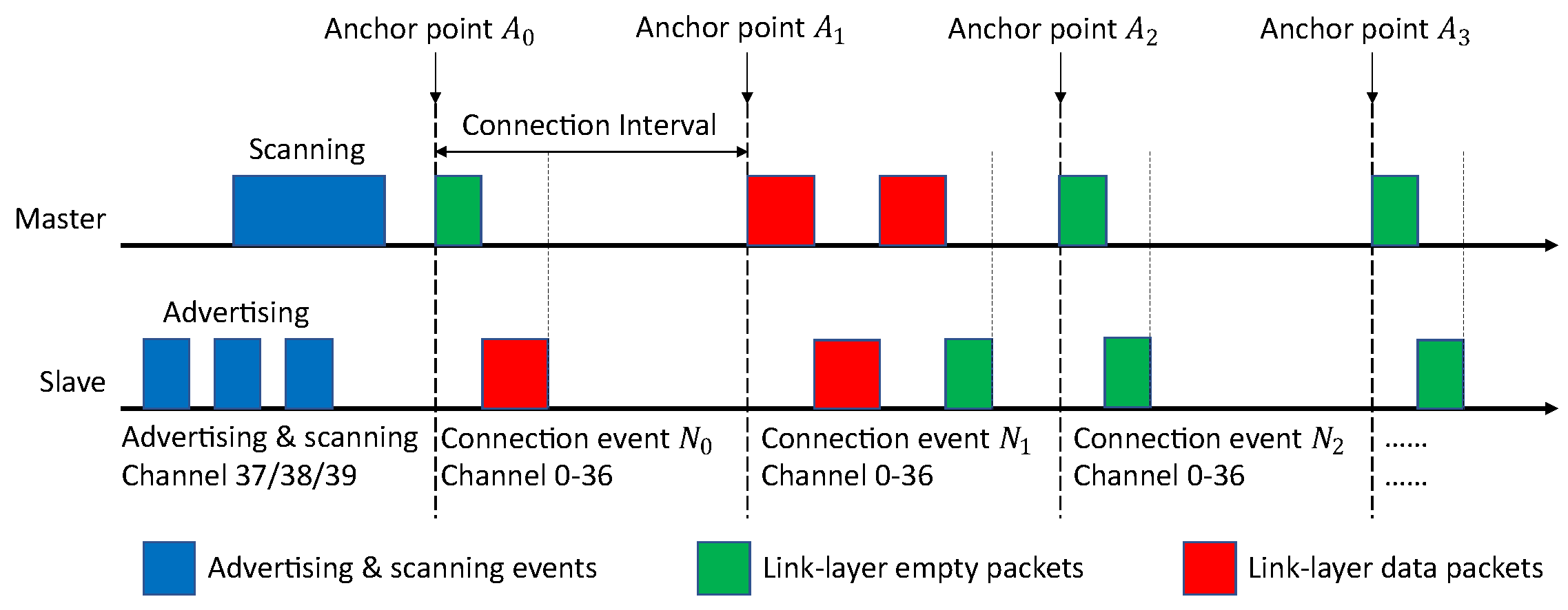
3.1. BLE Communication Process
3.2. Anchor Point
3.3. Acknowledgment
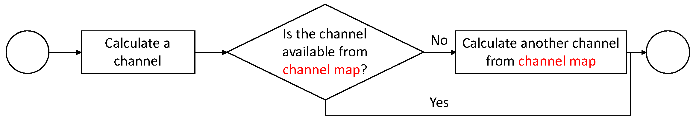
3.4. AFH and CSAs
3.5. Current Issues and Challenges
4. BLE Link Layer Robustness
4.1. Link Layer Parameters
4.1.1. Supervision Timeout Ratio
4.1.2. Packet Loss Rate
4.2. Case Analysis
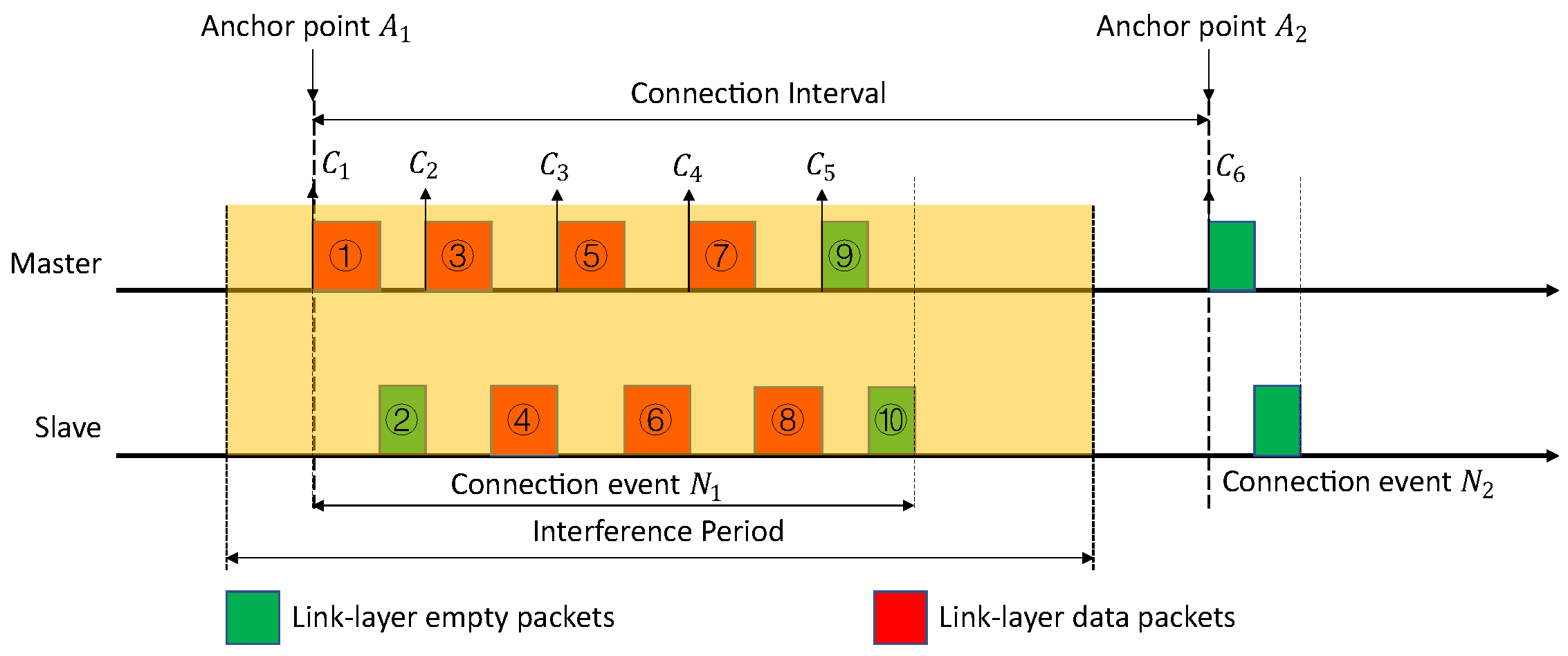
4.2.1. Case 1
- Assuming that packet ① is received successfully by the slave. At anchor point A1, the master sends the initial packet of connection event N1 to its slave. Since this packet ① is received successfully by the slave, the anchor point A1 is synchronized between the master and the slave. After packet ①, the slave will send packet ② back to the master. If the master receives this packet ② successfully, the STR and PLR can be calculated at point C2 according to the packets ① and ②.
- Assuming that packet ① is not received successfully by the slave. At anchor point A1, the master sends the initial packet of the connection event N1 to the slave. Since the packet ① is not received successfully by the slave, the anchor point A1 is therefore not synchronized. That leads to a failure of all the following packets, and packet ① is the only one left in the whole CI. In this situation, the STR rises at anchor point A1 or point C1. However, PLR cannot be calculated until the end of this CI, at anchor point A2 or point C6.
- Assuming that both packets ① and ② are transmitted successfully, and packet ③ is received by the slave without CRC or ACK errors. The slave starts to transmit packet ④. If this packet ④ is received by the master with CRC or ACK errors, the master will ask for a re-transmission from the slave. In this situation, both the STR and the PLR can be calculated at point C3. However, depending on the type of errors, only one of the results or both can tell the status of packet ③ and ④. Please note that, in BLE, there could be ACK errors with a correct CRC.
- Assuming that all the packets in the connection event N1 are successfully transmitted but partially correct. The connection event N1 ends with packet ⑩. The STR and the PLR are able to monitor every pair of data packets sent between the master and the slave. The STR is calculated from point C1 to C5. The PLR is calculated from C2 to C6. With both STR and PLR, the whole CI, from C1 to C6, is under monitoring.
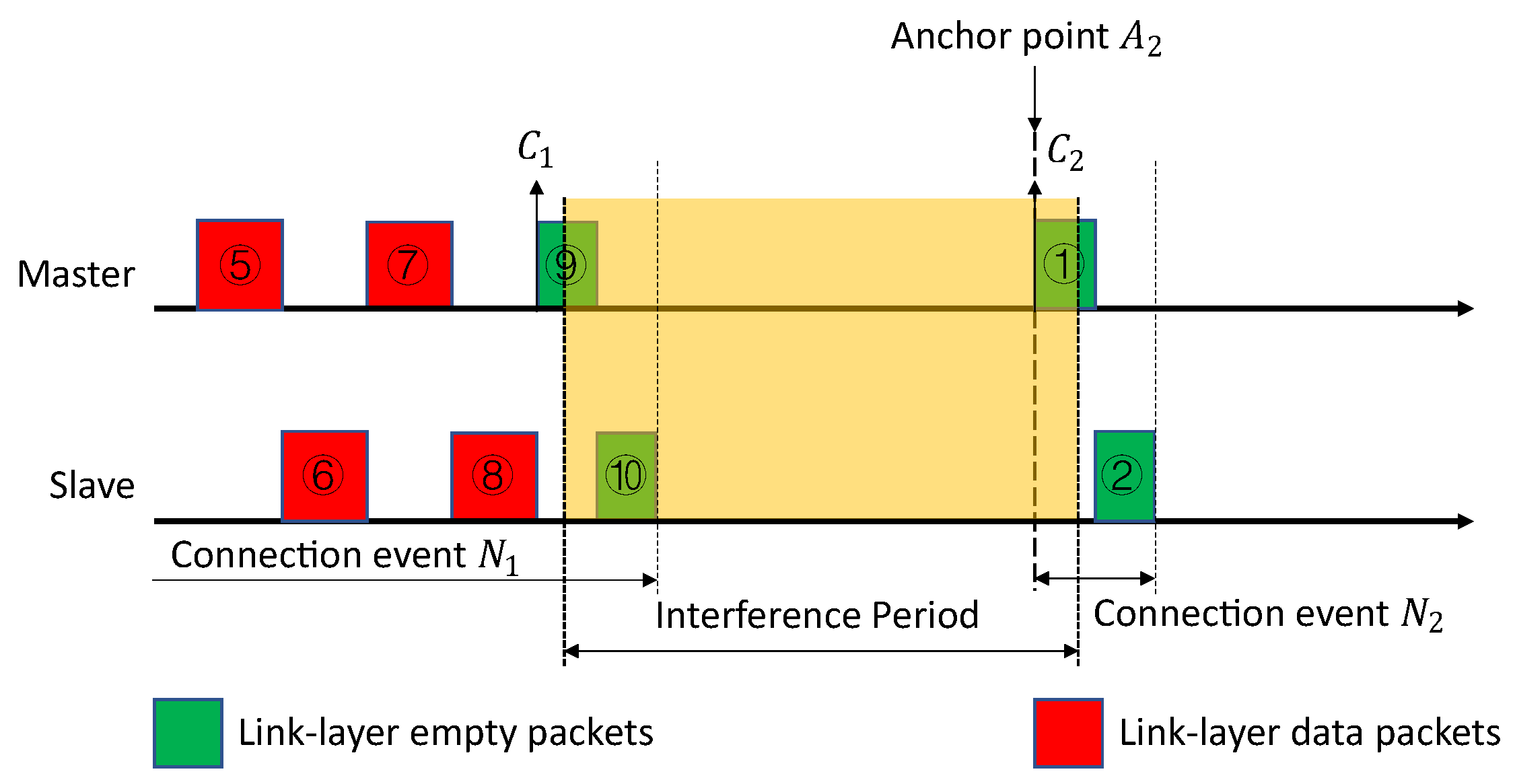
4.2.2. Case 2
- Assuming that packet ⑨ in connection event N1 is transmitted successfully and correctly. It does not matter if the packet ⑩ is transmitted successfully or not, at point C2, the PLR for the packets ⑨ and ⑩ in the connection event N1 is calculated. It can be used to show the transmission status and interference for the packets ⑨ and ⑩.
- Assuming that packet ① in connection event N2 is received successfully by the slave. The anchor point A2 is synchronized between the master and the slave. At point C2, the STR can be calculated for packet ① in the connection event N2. It can be used to show the anchor point synchronization status and interference for the packet ①. Under this situation, the PLR is not able to tell anything about the interference happening.
4.2.3. Analytical Results
5. IAS and Improved CSA
5.1. Interference Awareness Scheme (IAS)
| Algorithm 1: IAS |
 |
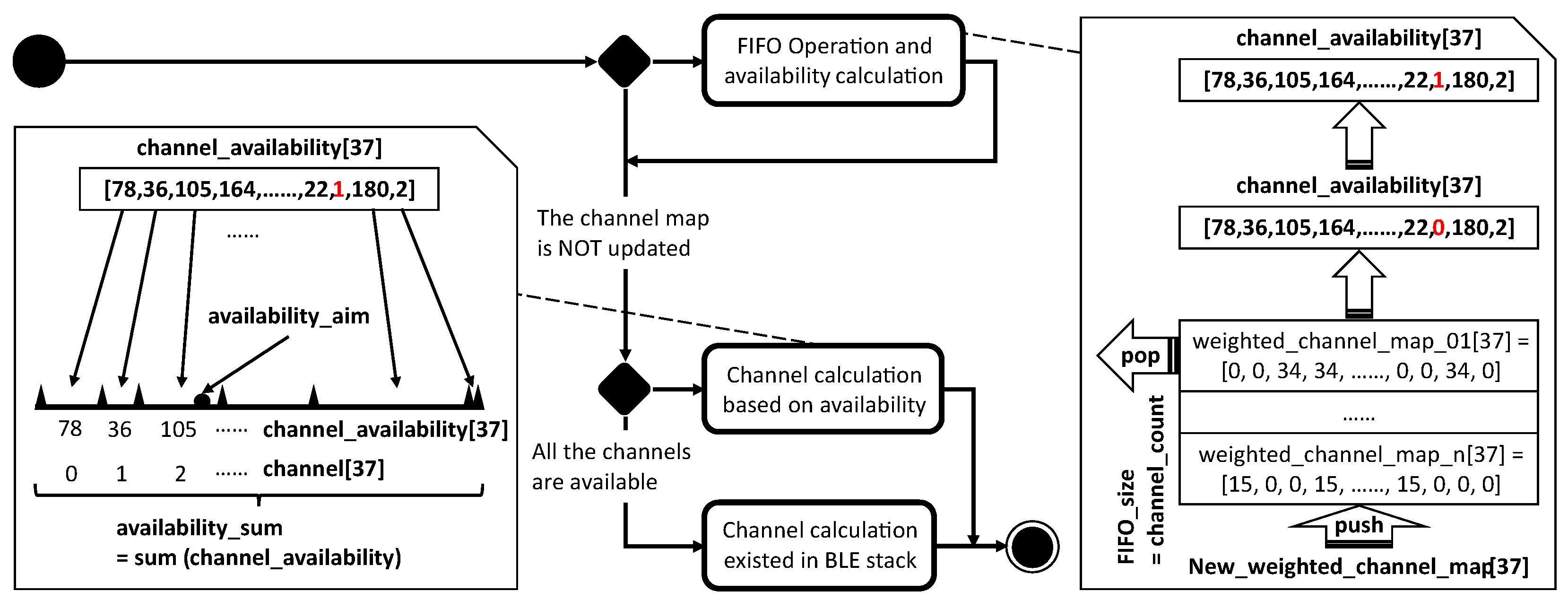
5.2. Improved CSA
| Algorithm 2: Improved CSA |
 |
6. Experiments and Results
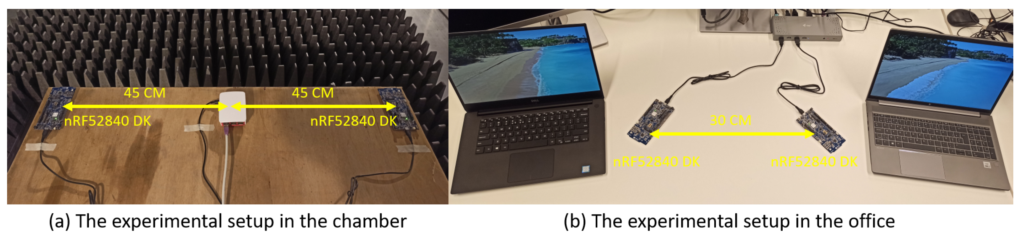
6.1. Experimental Setups
6.1.1. Controlled Environment
6.1.2. Uncontrolled Environment
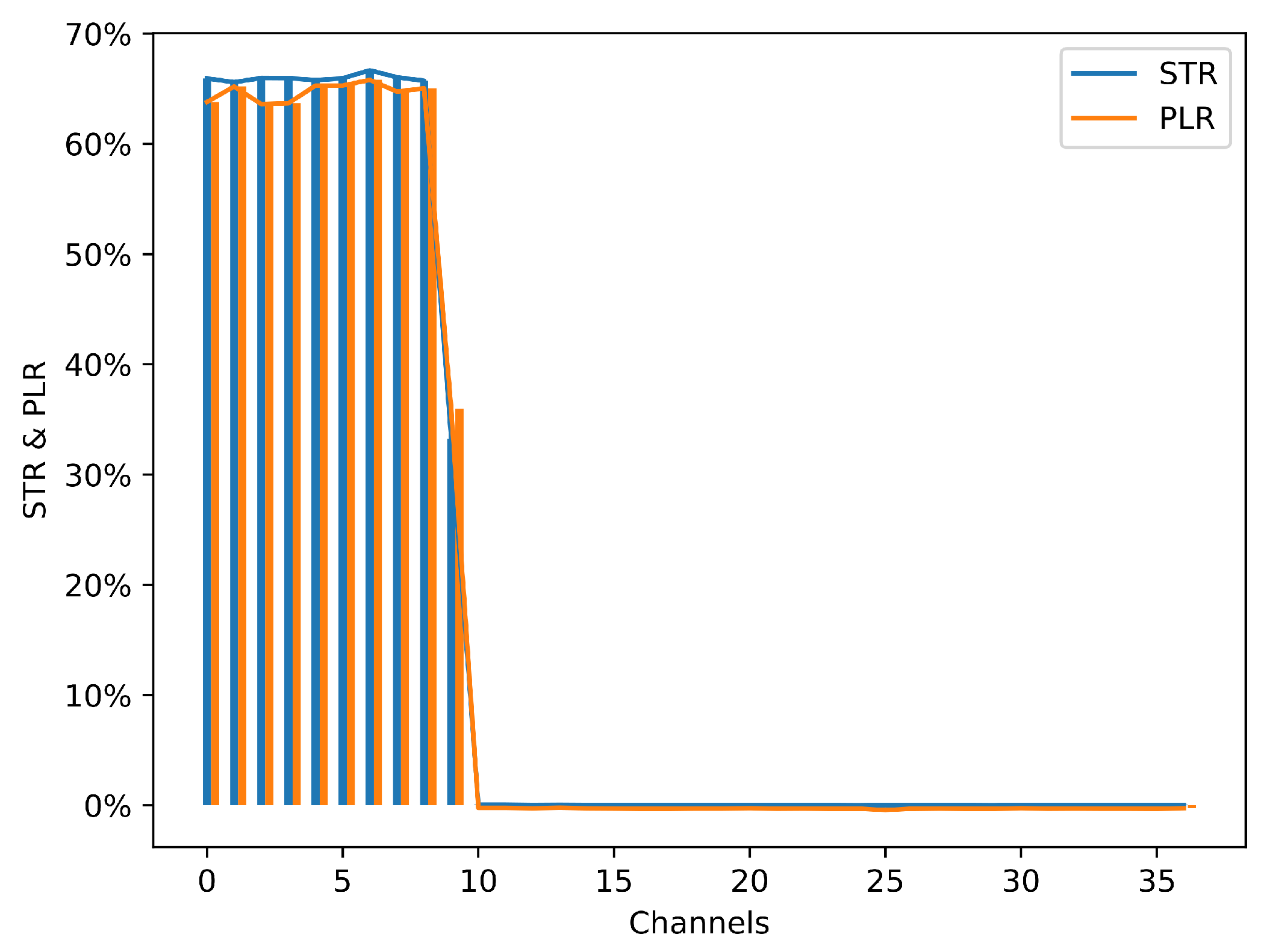
6.2. Channel Quality Baseline
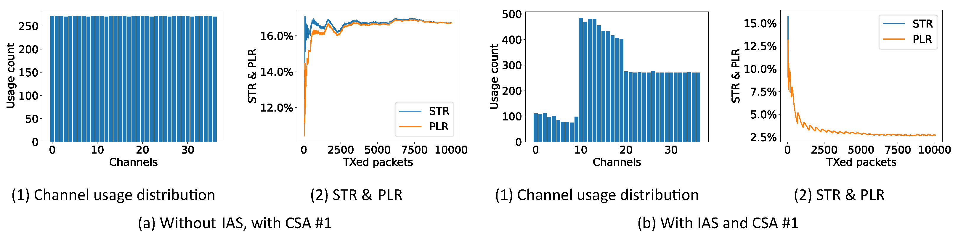
6.3. Feasibility of IAS in Existing CSAs
6.4. Experiments and Results of Combining the IAS with the Existing and Improved CSA
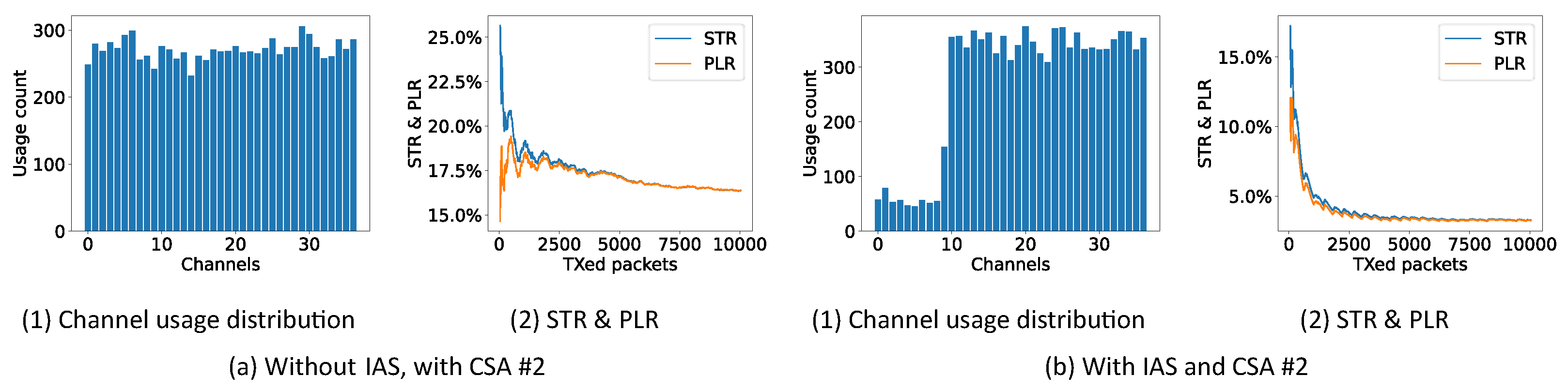
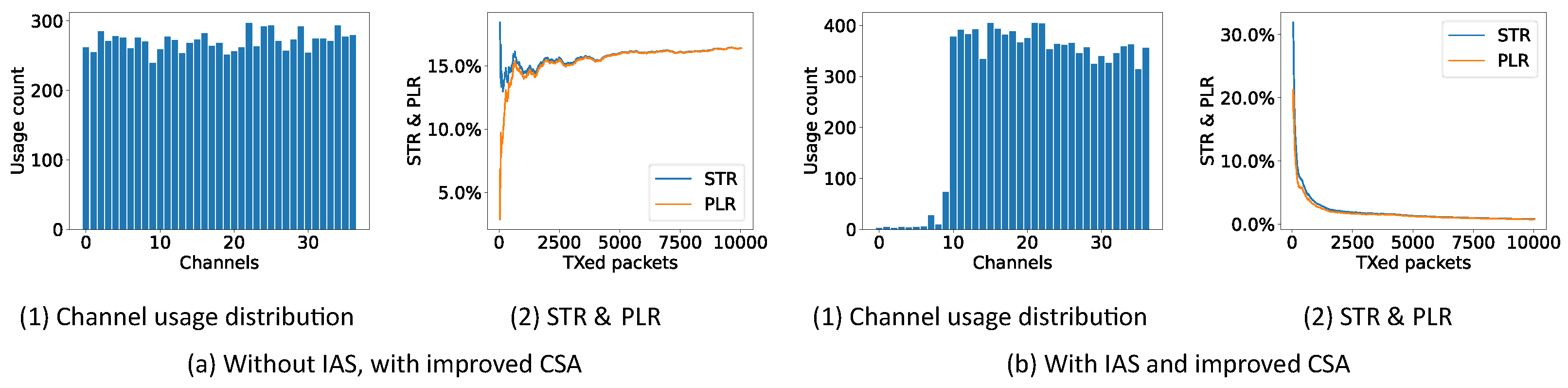
6.4.1. Controlled Fixed Interference
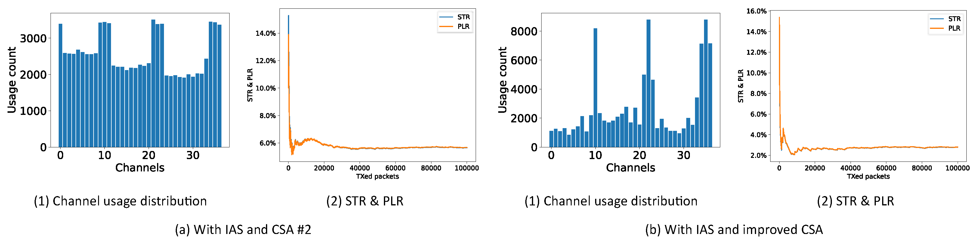
6.4.2. Controlled Random Interference
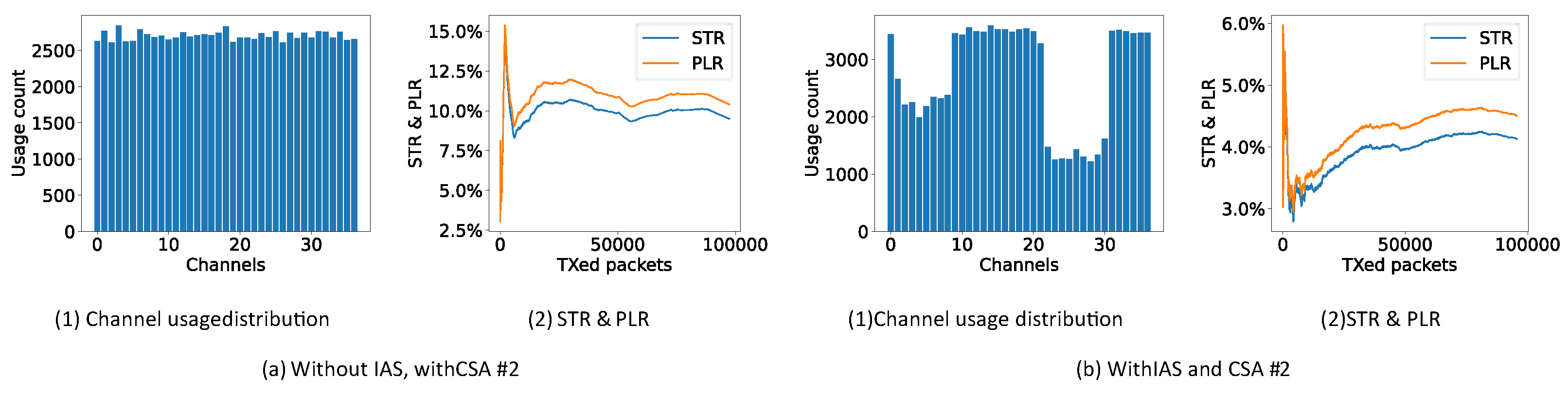
6.4.3. Uncontrolled Interference
6.4.4. Summary of the Experiments
6.4.5. Discussion for IAS and Improved CSA
7. Conclusions
Author Contributions
Funding
Institutional Review Board Statement
Informed Consent Statement
Conflicts of Interest
References
- Xie, C.; Yang, P.; Yang, Y. Open Knowledge Accessing Method in IoT-Based Hospital Information System for Medical Record Enrichment. IEEE Access 2018, 6, 15202–15211. [Google Scholar] [CrossRef]
- Peralta, G.; Iglesias-Urkia, M.; Barcelo, M.; Gomez, R.; Moran, A.; Bilbao, J. Fog computing based efficient IoT scheme for the Industry 4.0. In Proceedings of the 2017 IEEE International Workshop of Electronics, Control, Measurement, Signals and their Application to Mechatronics, ECMSM 2017, Donostia, Spain, 24–26 May 2017; pp. 1–6. [Google Scholar] [CrossRef]
- Natarajan, R.; Zand, P.; Nabi, M. Analysis of coexistence between IEEE 802.15.4, BLE and IEEE 802.11 in the 2.4 GHz ISM band. In Proceedings of the IECON (Industrial Electronics Conference), Florence, Italy, 23–26 October 2016; pp. 6025–6032. [Google Scholar] [CrossRef]
- Siekkinen, M.; Hiienkari, M.; Nurminen, J.K.; Nieminen, J. How low energy is bluetooth low energy? Comparative measurements with ZigBee/802.15.4. In Proceedings of the 2012 IEEE Wireless Communications and Networking Conference Workshops, WCNCW 2012, Paris, France, 1 April 2012; pp. 232–237. [Google Scholar] [CrossRef]
- Mikhaylov, K.; Plevritakis, N.; Tervonen, J. Performance analysis and comparison of bluetooth low energy with IEEE 802.15.4 and SimpliciTI. J. Sens. Actuator Netw. 2013, 2, 589–613. [Google Scholar] [CrossRef] [Green Version]
- Yun, S.; Son, H.; Hong, H.; Ahn, J. Throughput derivation for analysis of interference of the system with interference avoidance function in 2.4 GHz ISM band. In Proceedings of the International Conference on Advanced Communication Technology, ICACT, Gangwon, Korea, 13–16 February 2011; pp. 1119–1123. [Google Scholar]
- Kalaa, M.O.A.; Balid, W.; Bitar, N.; Refai, H.H. Evaluating Bluetooth Low Energy in realistic wireless environments. In Proceedings of the IEEE Wireless Communications and Networking Conference, WCNC, Doha, Qatar, 3–6 April 2016; pp. 1–6. [Google Scholar] [CrossRef]
- Bluetooth Special Interest Group. Bluetooth Core Specification v5.2; Bluetooth Special Interest Group: Kirkland, WA, USA, 2020. [Google Scholar]
- Bluetooth Special Interest Group. Bluetooth Core Specification v5.0; Bluetooth Special Interest Group: Kirkland, WA, USA, 2016. [Google Scholar]
- The Zephyr Project. Zephyr OS: An RTOS for IoT. 2020. Available online: https://zephyrproject.org/ (accessed on 23 March 2021).
- Rajpoot, V.; Tripathi, V.S. A Dedicated CCC based Data Channel Selection Scheme with Proactive Hand-off in Cognitive Radio Network. In Proceedings of the 2018 5th IEEE Uttar Pradesh Section International Conference on Electrical, Electronics and Computer Engineering, UPCON 2018, Gorakhpur, India, 2–4 November 2018; pp. 1–6. [Google Scholar] [CrossRef]
- Abbas, R.A.; Al-Sherbaz, A.; Bennecer, A.; Picton, P. A new channel selection algorithm for the weightless-n frequency hopping with lower collision probability. In Proceedings of the 2017 8th International Conference on the Network of the Future, NOF 2017, London, UK, 22–24 November 2017; pp. 171–175. [Google Scholar] [CrossRef] [Green Version]
- Ali, S.; Shokair, M.; Dessouky, M.I.; Messiha, N. Backup Channel Selection Approach for Spectrum Handoff in Cognitive Radio Networks. In Proceedings of the 2018 13th International Conference on Computer Engineering and Systems, ICCES 2018, Cairo, Egypt, 18–19 December 2018; pp. 353–359. [Google Scholar] [CrossRef]
- Desai Hinal, R.; Patel, N.B.; Suratwala, C.P. Channel and rate selection strategy in cognitive radio network using multi-arm bandits (MAB). In Proceedings of the 2018 3rd IEEE International Conference on Recent Trends in Electronics, Information and Communication Technology, RTEICT 2018, Bangalore, India, 18–19 May 2018; pp. 232–237. [Google Scholar] [CrossRef]
- Sengottuvelan, S.; Ansari, J.; Mahonen, P.; Venkatesh, T.G.; Petrova, M. Channel Selection Algorithm for Cognitive Radio Networks with Heavy-Tailed Idle Times. IEEE Trans. Mob. Comput. 2017, 16, 1258–1271. [Google Scholar] [CrossRef] [Green Version]
- Carhacioglu, O.; Zand, P.; Nabi, M. Cooperative Coexistence of BLE and Time Slotted Channel Hopping Networks. In Proceedings of the IEEE International Symposium on Personal, Indoor and Mobile Radio Communications, PIMRC, Bologna, Italy, 9–12 September 2018; pp. 1–7. [Google Scholar] [CrossRef]
- Nishio, Y.; Takyu, O.; Soya, H.; Ohta, M.; Fujii, T. Optimal Channel Selection Rate of Slave Terminal for Rendezvous Channel Scheme based on Channel Occupancy Rate. In Proceedings of the International Conference on Ubiquitous and Future Networks, ICUFN, Zagreb, Croatia, 2–5 July 2019; pp. 72–75. [Google Scholar] [CrossRef]
- Mathur, K.; Jena, D.; Agrawal, S.; Baburaj, S.; Kondabathini, S.; Tyagi, V. Throughput Improvement by Using Dynamic Channel Selection in 2.4 GHz Band of IEEE 802.11 WLAN. In Proceedings of the International Conference on Ubiquitous and Future Networks, ICUFN, Prague, Czech Republic, 3–6 July 2018; pp. 805–810. [Google Scholar] [CrossRef]
- Sumthane, M.Y.; Vatti, R.A. Wi-Fi interference detection and control mechanism in IEEE 802.15.4 wireless sensor networks. In Proceedings of the 2017 4th International Conference on Image Information Processing, ICIIP 2017, Shimla, India, 21–23 December 2017; pp. 496–501. [Google Scholar] [CrossRef]
- Ancans, A.; Ormanis, J.; Cacurs, R.; Greitans, M.; Saoutieff, E.; Faucorr, A.; Boisseau, S. Bluetooth Low Energy Throughput in Densely Deployed Radio Environment. In Proceedings of the 23rd International Conference Electronics 2019, ELECTRONICS 2019, Palanga, Lithuania, 17–19 June 2019; pp. 4–8. [Google Scholar] [CrossRef]
- Chek, M.C.H.; Kwok, Y.K. On adaptive frequency hopping to combat coexistence interference between bluetooth and IEEE 802.11b with practical resource constraints. In Proceedings of the International Symposium on Parallel Architectures, Algorithms and Networks, I-SPAN, Hong Kong, China, 10–12 May 2004; pp. 391–396. [Google Scholar] [CrossRef] [Green Version]
- Lee, W.; Kim, H. Channel Quality Estimation for Improving Awareness of Communication Situation in the 2.4 GHz ISM Band. IEEE Trans. Mob. Comput. 2018, 17, 2002–2013. [Google Scholar] [CrossRef]
- Spörk, M.; Boano, C.A.; Römer, K. Improving the Timeliness of Bluetooth Low Energy in Dynamic RF Environments. ACM Trans. Internet Things 2020, 1, 1–32. [Google Scholar] [CrossRef]
- Spörk, M.; Classen, J.; Boano, C.A.; Hollick, M.; Kay, R. Improving the Reliability of Bluetooth Low Energy Connections. In Proceedings of the International Conference on Embedded Wireless Systems and Networks (EWSN) 2020, Lyon, France, 17–19 February 2020; pp. 144–155. [Google Scholar]
- Freschi, V.; Lattanzi, E. A study on the impact of packet length on communication in low power wireless sensor networks under interference. IEEE Internet Things J. 2019, 6, 3820–3830. [Google Scholar] [CrossRef]
- Mucchi, L.; Carpini, A. ISM band aggregate interference in BAN-working environments. In Proceedings of the International Symposium on Medical Information and Communication Technology, ISMICT, Firenze, Italy, 2–4 April 2014; pp. 1–5. [Google Scholar] [CrossRef]
- Mikhaylov, K. Simulation of network-level performance for Bluetooth Low Energy. In Proceedings of the IEEE International Symposium on Personal, Indoor and Mobile Radio Communications, PIMRC, Washington, DC, USA, 2–5 September 2014; pp. 1259–1263. [Google Scholar] [CrossRef]
- Nordic Semiconductors. nRF52840 Specifications. 2020. Available online: https://www.nordicsemi.com/Software-and-Tools/Development-Kits/nRF52840-DK (accessed on 23 March 2021).
- Schuß, M.; Boano, C.A.; Weber, M.; Schulz, M.; Hollick, M.; Römer, K. JamLab-NG: Benchmarking Low-Power Wireless Protocols under Controllable and Repeatable Wi-Fi Interference. In Proceedings of the 2019 International Conference on Embedded Wireless Systems and Networks, EWSN ’19, Beijing, China, 25–27 February 2019. [Google Scholar]
- Hermeto, R.T.; Gallais, A.; Laerhoven, K.V.; Theoleyre, F. Passive Link Quality Estimation for Accurate and Stable Parent Selection in Dense 6TiSCH Networks. In Proceedings of the International Conference on Embedded Wireless Systems and Networks, EWSN 2018, Madrid, Spain, 12–16 February 2018; pp. 114–125. [Google Scholar]
- Al Kalaa, M.O.; Refai, H.H. Selection probability of data channels in Bluetooth Low Energy. In Proceedings of the 11th International Wireless Communications and Mobile Computing Conference, IWCMC 2015, Dubrovnik, Croatia, 24–28 August 2015; pp. 148–152. [Google Scholar] [CrossRef]
- Pang, B.Z.; Claeys, T.; Pissoort, D.; Hallez, H.; Boydens, J. Comparative study on AFH techniques in different interference environments. In Proceedings of the 2019 28th International Scientific Conference Electronics, ET 2019, Sozopol, Bulgaria, 12–14 September 2019; pp. 1–4. [Google Scholar] [CrossRef]
- Srinivasan, K.; Dutta, P.; Tavakoli, A.; Levis, P. An empirical study of low-power wireless. ACM Trans. Sens. Netw. 2010, 6, 1–49. [Google Scholar] [CrossRef] [Green Version]


| Parameters | Values |
|---|---|
| Hardware | nRF52840 DK |
| Software | Zephyr RTOS |
| Connection interval (CI) | 7.5 ms (30–50 ms by default, then updated to 7.5 ms) |
| Connection latency | 0 |
| Supervision timeout (ST) | 4 s |
| Maximum transmission unit | 23 bytes |
| PHY mode | LE 1M PHY |
| Connection Event | Channel Map | Number of Available Channels |
|---|---|---|
| 0 | [0xff, 0xff, 0xff, 0xff, 0x1f] | 37 |
| 30 | [0xff, 0xff, 0xff, 0xdf, 0x1f] | 36 |
| 38 | [0xfb, 0xff, 0xff, 0xdf, 0x1f] | 35 |
| 55 | [0xbb, 0xff, 0xff, 0xdf, 0x1f] | 34 |
| 59 | [0xbb, 0xfe, 0xff, 0xdf, 0x1f] | 33 |
| 62 | [0xb9, 0xfe, 0xff, 0xdf, 0x1f] | 32 |
| 69 | [0x39, 0xfe, 0xff, 0xdf, 0x1f] | 31 |
| 73 | [0x29, 0xfe, 0xff, 0xdf, 0x1f] | 30 |
| 83 | [0x21, 0xfe, 0xff, 0xdf, 0x1f] | 29 |
| 96 | [0x20, 0xfe, 0xff, 0xdf, 0x1f] | 28 |
| 102 | [0x00, 0xfe, 0xff, 0xdf, 0x1f] | 27 |
| …… | [……] | …… |
| 59642 | [0x00, 0x04, 0x00, 0x00, 0x01] | 2 |
| CSA #1 | CSA #2 | Improved CSA | ||
|---|---|---|---|---|
| fixed controlled Wi-Fi interference (after 10,000 connection events) | STR | 2.73% | 3.27% | 0.78% |
| PLR | 2.73% | 3.26% | 0.74% | |
| random controlled Wi-Fi interference (after 100,000 connection events) | STR | * | 5.65% | 2.78% |
| PLR | * | 5.65% | 2.80% | |
| uncontrolled Wi-Fi interference (after 100,000 connection events) | STR | * | 4.51% | 0.76% |
| PLR | * | 4.13% | 0.72% |
Publisher’s Note: MDPI stays neutral with regard to jurisdictional claims in published maps and institutional affiliations. |
© 2021 by the authors. Licensee MDPI, Basel, Switzerland. This article is an open access article distributed under the terms and conditions of the Creative Commons Attribution (CC BY) license (http://creativecommons.org/licenses/by/4.0/).
Share and Cite
Pang, B.; T’Jonck, K.; Claeys, T.; Pissoort, D.; Hallez, H.; Boydens, J. Bluetooth Low Energy Interference Awareness Scheme and Improved Channel Selection Algorithm for Connection Robustness. Sensors 2021, 21, 2257. https://0-doi-org.brum.beds.ac.uk/10.3390/s21072257
Pang B, T’Jonck K, Claeys T, Pissoort D, Hallez H, Boydens J. Bluetooth Low Energy Interference Awareness Scheme and Improved Channel Selection Algorithm for Connection Robustness. Sensors. 2021; 21(7):2257. https://0-doi-org.brum.beds.ac.uk/10.3390/s21072257
Chicago/Turabian StylePang, Bozheng, Kristof T’Jonck, Tim Claeys, Davy Pissoort, Hans Hallez, and Jeroen Boydens. 2021. "Bluetooth Low Energy Interference Awareness Scheme and Improved Channel Selection Algorithm for Connection Robustness" Sensors 21, no. 7: 2257. https://0-doi-org.brum.beds.ac.uk/10.3390/s21072257