Performance Analysis of Dual-Hop AF Relaying with Non-Linear/Linear Energy Harvesting

Abstract

Massive device-to-device communication nodes and Internet of Things (IoT) devices are expected to be crucial components in next-generation wireless networks. However, the energy constraint of these nodes presents a challenge since the energy of the batteries is limited. Motivated by this, radio frequency energy harvesting (EH) has been developed as an efficient strategy to overcome the energy constraint of IoT devices and sensor networks. In this paper, a wireless-powered dual-hop amplify-and-forward relaying system, in the absence of a direct link between the source (S) and the destination (D), is considered. It is assumed that a dedicated power beacon (PB) transmits an energy-bearing signal from which the power-constrained S and relay (R) harvest energy. Theoretical derivations of bit error probability, outage probability, and throughput expressions are performed for both linear and non-linear energy harvesting models. Moreover, the theoretical results provided for different system parameters are validated via Monte Carlo simulations. The obtained results reveal the difference between the realistic non-linear EH model and the conventional linear EH model, which overestimates the system performance at high levels of harvested energy. Thus, it leads to misunderstanding the real performance of the EH systems. However, at low levels of harvested energy, both models behave similarly and provide realistic results.

1. Introduction

By deploying massive sensor and Internet of Things (IoT) devices in next-generation wireless communication systems, energy limitation is revealed as one of the challenges for IoT devices. Normally, IoT devices are empowered by a battery, which limits their capacity and constrains their operational time. However, radio frequency (RF) EH can be an effective solution for empowering IoT devices, leading to increased operational time for battery-free IoT devices. In the literature, simultaneous wireless information and power transfer (SWIPT) and wireless-powered communication (WPC) schemes are considered as RF energy harvesting methods for the power-constrained nodes [1,2,3,4,5,6,7]. Power-splitting (PS) and time-switching (TS) are two EH receiver structures utilized in the SWIPT scheme. In PS EH mode, the power-constraint node harvests power from the incoming signal energy where one portion of the signal power is used for harvesting energy while the remainder is used for information processing. Moreover, in TS EH mode, two non-overlapping time intervals are dedicated to EH and IP, respectively. Moreover, the amount of harvested energy is considered as a linear or non-linear function of the energy receiving (ER) node input power [2,4,8,9,10,11,12,13,14].

Related Works

The system performance of power-constrained nodes considering the linear EH model is investigated in [15,16,17,18,19,20,21,22], where the harvested energy is a linear function of the received power at the battery-less node. However, due to the non-linearity of the EH circuit in practice, non-linear EH models are investigated in [23,24,25,26,27,28,29,30,31,32,33,34,35,36,37,38,39,40,41,42,43,44].

A massive multiple-input multiple-output (MIMO) relaying system with PS EH mode is investigated in an IoT cooperative network in [15]. The considered system’s achievable sum-rate is obtained for a relay which is power-constrained and harvests its power using the linear EH model. The system performance of power-constrained smart devices is investigated in [16], where a TS EH mode with the linear EH model is employed. A full-duplex (FD) dual-hop (DH) relaying network with the linear EH model is studied in [17]. Here, the power-constraint relay node applies PS and TS modes for EH purposes. Moreover, the relay forwards the source node signal to the destination, applying both amplify-and-forward (AF) and decode-and-forward (DF) relaying. Comprehensive throughput analyses of the considered system are performed for both the PS and TS EH modes. The throughput of the considered system is maximized for both PS and TS EH modes. The system performance of a cognitive IoT network with AF/DF relaying is investigated in [18], where the IoT network accesses the spectrum using orthogonal frequency-division multiplexing (OFDM). Moreover, the linear EH model with PS EH mode is considered in [18]. A cooperative non-orthogonal multiple access (NOMA) overlay spectrum sharing system with power-constrained secondary transmitters (STs) is examined in [19], where the STs operate in FD mode. Moreover, the outage probability and system throughput are investigated considering the linear EH model and PS EH mode. In [20], the outage probability of a cooperative DH relaying system with the linear EH model is derived where the TS EH mode is investigated. Here, the communication between the source and NOMA IoT devices is provided through power-constrained relay nodes.

Maximization of harvested energy in a non-convex problem is investigated in [23]. Here, an unmanned aerial vehicle (UAV) transfers power to the ground user location where the non-linear EH model is considered. The outage probability and throughput of a DH AF relaying two-way (TW) system are investigated in [24], where the relay harvests energy from both source nodes through the TS mode for the non-linear EH model. The throughput and ergodic capacity for a non-linear, piece-wise model are considered in [25], where a power-constrained source node harvests its power from the destination. The performance of a DH AF relaying system with a non-linear EH model is investigated in [26]. A closed-form expression for the bit error probability (BEP) is derived for binary differential phase-shift keying modulation, where the relay is assumed to be power-constrained. The performance of a cooperative AF relaying system is analyzed in [27]. The outage probability is investigated for perfect and imperfect channel state information (CSI), where the relay applies PS for the non-linear EH model. A massive MIMO SWIPT system’s energy efficiency is maximized in [28] where a base station transmits power, and the TS EH mode ratio is optimized. The spectral efficiency and average harvested energy of an FD DF relaying network with multiple users are investigated in [29].

The performance of an FD cognitive radio (CR) system for both linear and non-linear EH models is analyzed in [30]. It is assumed that the secondary transmitter is power-constrained and harvests its energy from both the primary transmitter (PT) and the secondary receiver. The bit error rate (BER) performance for both primary and secondary users is derived for different system parameters. The performance of a multi-antenna FD CR EH system is investigated in [31], where the transmitter employs the NOMA technique to transmit from the PT. Both the throughput and the outage probability of the system based on the non-linear EH model are investigated. In [32], the system performance of a cooperative NOMA network, which consists of three nodes, is analyzed. The near user is considered to be power-constrained and harvests its power from the incoming source signal. The outage probability of an overlay CR is considered in [33]. It is assumed that the secondary user is power-constrained and harvests its energy from the PT signal. The system performance of a DH DF relaying system with multiple power-constrained relays is investigated in [34]. A closed-form outage probability expression is derived considering the TS EH protocol. A cooperative DF relaying network with spectrum sensing and an ER node is examined in [35]. The power-constrained node simultaneously harvests energy and processes information by applying the PS technique.

A MIMO wireless power transfer ER architecture design is studied in [36]. The total harvested power is maximized for the proposed generic architecture of multiple ER nodes. The rate-energy trade-off of a point-to-point SWIPT system with a non-linear EH model is investigated in [37]. The ergodic fading channel is considered in [37] where the power-constrained node applies the PS EH mode. The sum throughput of the relay-based wireless-powered system is investigated in [38]. The relay adopts the non-linear EH model to harvest power from a dedicated power beacon. The sum throughput is maximized jointly considering a non-convex problem with parameters of power and time fraction. A non-linear EH model for a device-to-device network is proposed in [39]. In this study, the energy efficiency is maximized, considering the PS EH mode of the IoT nodes by optimizing the resource and power allocation. A WPC network with a non-linear EH model is investigated in [40], where the weighted sum of computation bits in each user is maximized for the considered non-convex optimization problem. A cooperative DH AF relaying system with a mixed fading environment and a non-linear EH model is investigated in [41]. Here, it is assumed that the relay is power-constrained and harvests its power from the source using PS/TS EH modes. The system performance of a MIMO IoT network in the presence of cooperative jamming is considered in [42], where a non-linear EH model with PS protocol is assumed. In [43], the non-linear EH model is applied to UAV-assisted FD IoT networks, where infinite and finite blocklength codes are considered. The performance of the system is analyzed in terms of the block error rate, where the theoretical derivation is performed considering Rician shadowed fading channels. Our study can be extended for finite blocklength considering [43] and references therein.

2. Methods

In this paper, the theoretical expressions for the bit error probability (BEP) and the throughput of a wireless-powered dual-hop amplify-and-forward (WP DH AF) relaying system are considered. Moreover, we investigate a non-linear piece-wise EH model which is mathematically tractable in terms of the PDF, CDF of harvested power, and the system performance. Apart from the linear EH model described in the literature, this model provides practical performance analyses. Specifically, the non-linear EH model considered in [8,11,26,27,34,45] is addressed since this model is mathematically tractable compared to other non-linear EH models [9,10,12,13]. In contrast to the linear EH model, which overestimates system performance, the considered non-linear piece-wise EH model provides realistic system performance along with the practical non-linear EH models. Since most papers in the literature have considered the linear EH model, in this paper, the effect of the linear EH model is investigated along with the non-linear piece-wise EH model, to provide a comprehensive system analysis. Hence, comparisons of linear and non-linear EH models are also provided. To the best of the authors’ knowledge, the BEP, outage probability, and throughput of the considered system have not yet been investigated in the literature. The contributions of this paper are summarized as follows:

• Theoretical derivation of BEP expressions considering both linear and non-linear EH models is performed.
• Throughputs of the considered system for both linear and non-linear EH models are derived.
• Simulation and theoretical results of the considered system are provided for different system parameters, such as distance, power, and achievable rate.

The paper is organized as follows: The system model is described in Section 3. Theoretical BEP derivations are provided in Section 4. Section 5 deals with the throughput analysis. Numerical results are presented in Section 6. Finally, Section 7 concludes the paper.

3. System Model

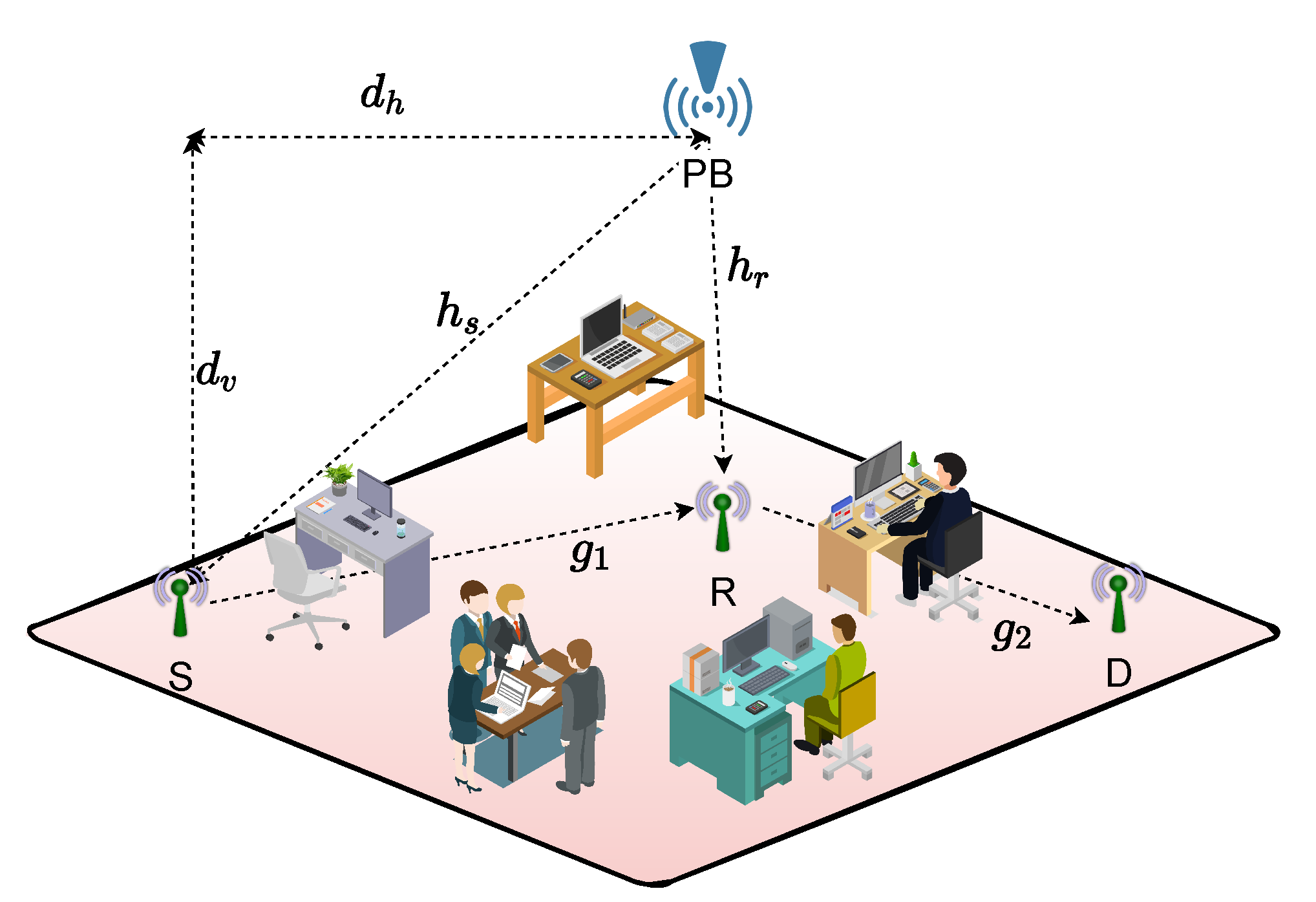
The DH AF relaying system under consideration is given in Figure 1, where the source (S) and relay (R) are power-constrained nodes and harvest their energy from a dedicated power beacon (PB). Hence, S and R use their harvested powers for data transmission. In the absence of a direct link between S and the destination (D), the communication is provided with the help of R. All nodes are equipped with only one antenna.

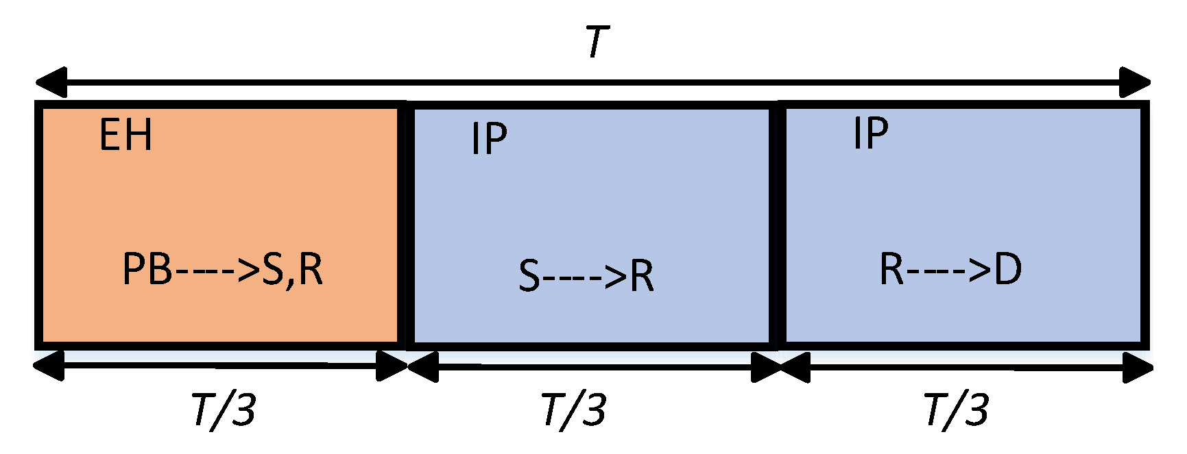
A typical RF EH process is achieved in a short range and a line of sight (LoS) exists between PB and the EH nodes. Inspired by this fact, we assume that the links between nodes in Figure 1 are exposed to mix-fading [30,46]. The proper fading channel model, including an LoS component, is considered as the Rician model. However, the cumulative distribution function (CDF) and probability distribution function (PDF) of the Rician distribution include special functions which make the analysis more complicated and the results are not mathematically tractable. On the other hand, the Nakagami-m fading model provides a good approximation of the Rician channel model [47,48,49]. Motivated by this, we assume that the links PB→S and PB→R are exposed to Nakagami-m fading, represented by channel coefficients $h_s$ and $h_r$, with channel parameters $m_z$ and $m_w$, respectively. Moreover, the links S→R and R→D are subject to Rayleigh fading, with gains $g_1$ and $g_2$, respectively. It is assumed that the CSI is perfectly known at the receiving nodes, and the channels are assumed to be exposed to flat fading and remain fixed during a transmission interval and vary independently from one interval to another. The overall transmission time T is divided into three equal time slots, as shown in Figure 2. It should be noted that this assumption is considered in [2,4] where it provides a maximized system performance. In the first time slot of duration $T/3$, PB broadcasts the dedicated energy bearing signal. In the second and third time slots, S and R transmit their signals to R and D, respectively. $n_r$ and $n_d$ denote additive white Gaussian noise (AWGN) samples which are independent and identically distributed (i.i.d.) complex Gaussian random variables (r.v) as $n_r,n_d\sim \mathcal{C}\mathcal{N}(0,N_0)$. Finally, the notation and system parameters are listed in

Table 1. List of notations.

Notation	Description
$\Gamma (·,·)$	Upper incomplete Gamma function ([50], 8.350)
$F_{·}(·)$	Cumulative distribution function (CDF)
$f_{·}(·)$	Probability distribution function (PDF)
$\Gamma (·)$	Gamma function ([50], 8.310).
$\gamma (·,·)$	Lower incomplete Gamma function ([50], 8.350)
${(·)}_{·}$	Pochhammer’s symbol ([51], 6.1-22)
${}_1{F}_1\left(·;·;·\right)$	Kummer Confluent Hyper-geometric function ([52], 07.20.07.0001.01)
$G\begin{array}{c}mn\\ pq\end{array}\left(·|\begin{array}{c}{a}_p\\ b_q\end{array}\right)$	Meijer-G function ([50], 9.301)
${\mathrm{K}}_x(·)$	Modified Bessel function of the second kind with order x [50]

and

Table 2. List of parameters.

Parameters	Description
$P_T$	PB transmit power
${\eta }_s$	Energy conversion coefficient $(0<{\eta }_s<1)$
${\eta }_r$	Energy conversion coefficient $(0<{\eta }_r<1)$
$P_s$	Harvested power at node S
$P_r$	Harvested power at node R
x	Transmitted signal from S with $\mathrm{E}\left\{\right|x{|}^2\}=1$
$a,b$	Modulation specific constants [4]
${\Omega }_{h_i}=\mathrm{E}\left\{\right|h_i{|}^2\}$	Channel fading gains, $i\in \{s,r\}$
${\Omega }_{g_j}=\mathrm{E}\left\{\right|g_j{|}^2\}$	Channel fading gains, $j\in \{1,2\}$
$P_{t{h}_i}$	Threshold (saturation) power at source and relay nodes $i\in \{s,r\}$
$\nu$	Path loss exponent
$L_i=1/\sqrt{1+d_i^{\nu }}$	Pathloss $i\in \{st,rt,sr,rd\}$ [1,4]
$d_{sr}$	S→R link distance
$d_{rd}$	R→D link distance
$d_{st}$	Distances from PB to S
$d_{rt}$	Distances from PB to R
$d_v$	Vertical distance from PB to node S
$d_h$	Horizontal distance from S to PB
$N_0$	Noise power spectral density
$\vartheta ={log}_{2}M$	Number of bits per symbol
M	Modulation order

, respectively.

Linear and Non-Linear EH Models

In the literature, two EH models are considered: linear and non-linear. In the linear EH model, the transmit power of the power-constrained node is increased by increasing the harvested power at the considered node [2,4]. This causes a misrepresentation of the amount of harvested power [53] since, in practical EH circuits, the amount of the harvested power increases to a threshold level rather than the considered amount of harvested power in the linear EH model.

In other words, in practice, due to the non-linear behavior of the diodes in EH circuits, non-linear EH models are more realistic compared to the linear EH model. Additionally, a maximum threshold power is defined for the non-linear EH model, such that, for harvested power greater than this threshold value, the transmit powers of S and R take this fixed threshold value [8,9,10,11,12,13]. Specifically, we assume the non-linear EH model given in [8,11] since the non-linear EH models proposed in [9,10,12,13] are not mathematically tractable. Moreover, the considered model provides a good approximation of practical EH circuits at low and high amounts of harvested power [8,53] which broadens the insight of EH system design along with the well-studied linear EH model.

In the first time slot, S and R harvest energy from PB. For the linear EH model, the harvested power for S and R is given as [2]

$$\begin{array}{c}\hfill P_i=P_{h_i}={\eta }_i{P}_T{L}_{it}{\left|h_i\right|}^2,\end{array}$$

(1)

where $P_{h_i}$ is the harvested power at node i with $i\in \{s,r\}$. However, assuming the non-linear EH model, the harvested power at S and R is given as [8,11]

$$P_i=\left\{\begin{array}{cc}{P}_{h_i},\hfill & P_{h_i}\le P_{t{h}_i}\hfill \\ P_{t{h}_i},\hfill & P_{h_i}>P_{t{h}_i},\hfill \end{array}\right.$$

(2)

where $i\in \{s,r\}$. We assume that all of the harvested energy at both nodes S and R during the first time slot of $T/3$ is consumed for the transmission of the signal x in the consecutive time slots of each $T/3$ since there is no available energy buffer at the power-constrained nodes. Moreover, high input power is limited to the threshold power $P_{t{h}_i}$. In thesecond time slot, the received signal at node R is

$$\begin{array}{c}\hfill y_r=\sqrt{P_s{L}_{sr}}{g}_{1}x+n_r.\end{array}$$

(3)

In the third time slot, R forwards the amplified version of the received signal in (3). The received signal at D is then given as

$$\begin{array}{c}\hfill y_d=\sqrt{{\displaystyle \frac{P_r{L}_{rd}}{G}}}{g}_2{y}_r+n_d,\end{array}$$

(4)

where $G=\mathrm{E}\left\{\right|y_r{|}^2\}=P_s{L}_{sr}{\left|g_1\right|}^2+N_0$ is the normalization factor. Substituting (3) in (4), we have

$$\begin{array}{c}\hfill y_d=\sqrt{{\displaystyle \frac{P_s{P}_r{L}_{sr}{L}_{rd}}{G}}}{g}_1{g}_{2}x+\sqrt{{\displaystyle \frac{P_r{L}_{rd}}{G}}}{g}_2{n}_r+n_d.\end{array}$$

(5)

The received SNR at D is calculated from (5) as

$$\begin{array}{c}\hfill \gamma ={\displaystyle \frac{XY}{X+Y+1}}\le \min (X,Y),\end{array}$$

(6)

where $X=Z{X}^{\prime }$, $Y=W{Y}^{\prime }$ and we assume a tight upper bound in (6). For simplicity, we assume $Z=P_s$, $W=P_r$, $X^{\prime }=L_{sr}{\left|g_1\right|}^2/N_0$ and $Y^{\prime }=L_{rd}{\left|g_2\right|}^2/N_0$. In addition, $Z\sim \Gamma (m_z,{\varphi }_z)$ and $W\sim \Gamma (m_w,{\varphi }_w)$ are Gamma distributed r.v.s with parameters $m_z$ and $m_w$, respectively, and the scaling parameters are ${\varphi }_z=m_z/\overline{z}$ and ${\varphi }_w=m_w/\overline{w}$. Moreover, $\overline{z}={\eta }_s{P}_T{L}_{st}{\Omega }_{h_s}$ and $\overline{w}={\eta }_r{P}_T{L}_{rt}{\Omega }_{h_r}$. Furthermore, $X^{\prime }$ and $Y^{\prime }$ are exponentially distributed as $\mathrm{Exp}\left({\overline{x}}^{\prime }\right)$ and $\mathrm{Exp}\left({\overline{y}}^{\prime }\right)$, where ${\overline{x}}^{\prime }=L_{sr}{\Omega }_{g_1}/N_0$ and ${\overline{y}}^{\prime }=L_{rd}{\Omega }_{g_2}/N_0$, respectively.

In (6), using ([54], eq. 6-81), the conditioned CDF of $\gamma$ is expressed as

$$\begin{array}{c}\hfill F_{\gamma }\left(\gamma \right|Z,W)=F_X\left(\gamma \right|Z)+F_Y\left(\gamma \right|W)-F_X\left(\gamma \right|Z)F_Y\left(\gamma \right|W),\end{array}$$

(7)

where

$$\begin{array}{cc}\hfill & F_X\left(\gamma \right|Z)=1-exp(-\frac{\gamma }{Z{\overline{x}}^{\prime }}),\hfill \end{array}$$

(8)

$$\begin{array}{cc}\hfill & F_Y\left(\gamma \right|W)=1-exp(-\frac{\gamma }{W{\overline{y}}^{\prime }}).\hfill \end{array}$$

(9)

Substituting both (8) and (9) in (7) and simplifying, the conditioned CDF in (7) is obtained as

$$\begin{array}{c}\hfill F_{\gamma }\left(\gamma \right|Z,W)=1-exp(-\gamma (\frac{1}{Z{\overline{x}}^{\prime }}+\frac{1}{W{\overline{y}}^{\prime }})).\end{array}$$

(10)

4. BEP Analysis

In this section, the BEP of the considered DH AF relaying system is derived for both non-linear and linear EH models. In order to obtain the BEP expression, the analytical expression of symbol error probability (SEP) is first derived. The overall BEP expression is given for high SNR, assuming the common approximation for Gray mapping [55] as $P_b^i\approxeq P_s^i/\vartheta$. Here, $i\in \{\mathrm{L},\mathrm{NL}\}$, L and NL represent linear and non-linear EH models, respectively. The conditioned SEP for both linear and non-linear EH models is calculated as [4]

$$\begin{array}{c}\hfill P_s^{L,NL}\left(e\right|Z,W)={\displaystyle \frac{a\sqrt{b}}{2\sqrt{\pi }}}{\int }_0^{\infty }{\displaystyle \frac{e^{-b\gamma }}{\sqrt{\gamma }}}{F}_{\gamma }\left(\gamma \right|Z,W)\mathrm{d}\gamma ={\displaystyle \frac{a\sqrt{b}}{2\sqrt{\pi }}}(I_1-I_2(Z,W)),\end{array}$$

(11)

where parameters a and b denote the modulation coefficients for M-PSK/QAM [4] and $F_{\gamma }\left(\gamma \right|Z,W)$ is given in (10). In (11),

$$\begin{array}{c}\hfill I_1={\int }_0^{\infty }{\displaystyle \frac{e^{-b\gamma }}{\sqrt{\gamma }}}\mathrm{d}\gamma =\sqrt{{\displaystyle \frac{\pi }{b}}}\end{array}$$

(12)

and

$$\begin{array}{c}\hfill I_2(Z,W)={\int }_0^{\infty }{\displaystyle \frac{1}{\sqrt{\gamma }}}exp(-\gamma (b+\frac{1}{Z{\overline{x}}^{\prime }}+\frac{1}{W{\overline{y}}^{\prime }}))\mathrm{d}\gamma =\sqrt{{\displaystyle \frac{\pi }{b+\frac{1}{Z{\overline{x}}^{\prime }}+\frac{1}{W{\overline{y}}^{\prime }}}}}\end{array}$$

(13)

which are calculated using ([50], eq. 3.361-2). After substituting (12) and (13) and simplifying, (11) is obtained as

$$\begin{array}{cc}\hfill P_s^{L,NL}\left(e\right|Z,W)& ={\displaystyle \frac{a}{2}}\left[1-{\displaystyle \frac{1}{\sqrt{1+\frac{1}{Z\overline{x}}+\frac{1}{W\overline{y}}}}}\right],\hfill \end{array}$$

(14)

where $\overline{x}=b{\overline{x}}^{\prime }$ and $\overline{y}=b{\overline{y}}^{\prime }$.

4.1. BEP Analysis of the Non-Linear EH Model

In this subsection, the BEP of the non-linear EH model is derived analytically. The overall BEP for the non-linear EH model is expressed as

$$\begin{array}{c}\hfill P_b^{NL}\approxeq (P_{s1}+P_{s2}+P_{s3}+P_{s4})/\vartheta ,\end{array}$$

(15)

where $P_{s1}$, $P_{s2}$, $P_{s3}$, and $P_{s4}$ stand for the four states of power harvesting processes considering both nodes S and R, which are calculated as

$$\begin{array}{cc}\hfill & P_{s1}={\int }_{w=0}^{P_{th}}\underset{A\left(w\right)}{\underbrace{{\int }_{z=0}^{P_{th}}{P}_s^{L,NL}\left(e\right|z,w)f_Z\left(z\right)\mathrm{d}z}}{f}_W\left(w\right)\mathrm{d}w,\hfill \end{array}$$

(16)

$$\begin{array}{cc}\hfill & P_{s2}=P_s^{L,NL}(e|\begin{array}{c}z=P_{th}\\ w=P_{th}\end{array})\underset{B_1}{\underbrace{{\int }_{w=P_{th}}^{\infty }{f}_W\left(w\right)\mathrm{d}w}}\underset{B_2}{\underbrace{{\int }_{z=P_{th}}^{\infty }{f}_Z\left(z\right)\mathrm{d}z}},\hfill \end{array}$$

(17)

$$\begin{array}{cc}\hfill & P_{s3}=\underset{A_1{=A\left(w\right)|}_{w=P_{th}}}{\underbrace{{\int }_{z=0}^{P_{th}}{P}_s^{L,NL}\left(e\right|z,w)f_Z\left(z\right)\mathrm{d}z}}\underset{B_1}{\underbrace{{\int }_{w=P_{th}}^{\infty }{f}_W\left(w\right)\mathrm{d}w}},\hfill \end{array}$$

(18)

and

$$\begin{array}{cc}\hfill & P_{s4}=\underset{A_2{=A\left(z\right)|}_{z=P_{th}}}{\underbrace{{\int }_{w=0}^{P_{th}}{P}_s^{L,NL}\left(e\right|z,w)f_W\left(w\right)\mathrm{d}w}}\underset{B_2}{\underbrace{{\int }_{z=P_{th}}^{\infty }{f}_Z\left(z\right)\mathrm{d}z}}.\hfill \end{array}$$

(19)

$A\left(w\right)$, and $P_{s1}$ in (16) and $A\left(z\right)$ in (19) are calculated in Appendix A, Appendix B, and Appendix C, respectively.

In (19), $A_2$ is calculated from (A29) as $A_2{=A\left(z\right)|}_{z=P_{th}}$. Furthermore, using ([50], eq. 3.351-2), $B_2$ in (19) is calculated as

$$\begin{array}{c}\hfill B_2={\int }_{P_{th}}^{\infty }{f}_Z\left(z\right)\mathrm{d}z=D\Gamma (m_z,P_{th}{\varphi }_z)/{\varphi }_z^{m_z},\end{array}$$

(20)

where

$$\begin{array}{c}\hfill f_Z\left(z\right)=D{z}^{m_z-1}exp(-z{\varphi }_z)\end{array}$$

(21)

with $D={\varphi }_z^{m_z}/\Gamma \left(m_z\right)$. Finally, $P_{s4}$ in (19) is calculated by substituting $A_2{=A\left(z\right)|}_{z=P_{th}}$ in (A29) and (20).

In (19), $A_1$ is calculated from (A2) as $A_1{=A\left(w\right)|}_{w=P_{th}}$. Moreover, using ([50], 3.351-2), $B_1$ in (18) is calculated as

$$\begin{array}{c}\hfill B_1={\int }_{P_{th}}^{\infty }{f}_W\left(w\right)\mathrm{d}w=I\Gamma (m_w,P_{th}{\varphi }_w)/{\varphi }_w^{m_w},\end{array}$$

(22)

where

$$\begin{array}{c}\hfill f_W\left(w\right)=I{w}^{m_w-1}exp(-w{\varphi }_w)\end{array}$$

(23)

with $I={\varphi }_w^{m_w}/\Gamma \left(m_w\right)$. Moreover, $P_{s3}$ in (18) is calculated by substituting $A_1{=A\left(w\right)|}_{w=P_{th}}$ in (A2) and (22). Finally, $P_{s2}$ in (17) is calculated using (22), (20), and replacing $z=P_{th}$ and $w=P_{th}$ in (14).

4.2. Linear EH Model

In this subsection, the BEP of the considered DH AF relaying system is derived for the linear EH. Here, it is assumed that the harvested energy is linearly dependent on the received energy and increases by increasing the energy transferred from PB. At high SNR values, the overall BEP for the linear EH model is given as

$$\begin{array}{c}\hfill P_b^L\approxeq \frac{1}{\vartheta }{\int }_0^{\infty }\underset{P_s\left(e\right|w)}{\underbrace{{\int }_0^{\infty }{P}_s^{L,NL}\left(e\right|z,w)f_Z\left(z\right)\mathrm{d}z}}{f}_W\left(w\right)\mathrm{d}w.\end{array}$$

(24)

In (24), $P_s\left(e\right|w)$ is calculated by substituting $f_Z\left(z\right)$ and $P_s^{L,NL}\left(e\right|z,w)$ from (21) and (14) as

$$\begin{array}{c}\hfill P_s\left(e\right|w)={\displaystyle \frac{a}{2}}(E_0-F_0\left(w\right)),\end{array}$$

(25)

where

$$\begin{array}{c}\hfill E_0={\int }_0^{\infty }{f}_Z\left(z\right)\mathrm{d}z=1,\end{array}$$

(26)

and after simplifying

$$\begin{array}{c}\hfill F_0\left(w\right)=\frac{D}{\sqrt{B}}{\int }_0^{\infty }{\displaystyle \frac{z^{m_z-0.5}}{\sqrt{1+z/G}}}exp(-z{\varphi }_z)\mathrm{d}z,\end{array}$$

(27)

where $G=B/C$. Using ([56], eq. 10), (27), is rewritten as

$$\begin{array}{c}\hfill F_0\left(w\right)=\frac{D}{\Gamma \left(0.5\right)\sqrt{B}}{\int }_0^{\infty }{z}^{m_z-0.5}G\begin{array}{c}11\\ 11\end{array}\left({\displaystyle \frac{Z}{G}}|\begin{array}{c}0.5\\ 0\end{array}\right)exp(-z{\varphi }_z)\mathrm{d}z.\end{array}$$

(28)

Using ([50], eq. 7.813-1), and substituting $G=B/C$, (28) is obtained as

$$\begin{array}{c}\hfill F_0\left(w\right)=\frac{D}{\Gamma \left(0.5\right)\sqrt{B}}{\varphi }_z^{-(m_z+0.5)}G\begin{array}{c}12\\ 21\end{array}\left({\displaystyle \frac{1+w\overline{y}}{B{\varphi }_{z}w\overline{y}}}|\begin{array}{c}0.5-m_z,0.5\\ 0\end{array}\right).\end{array}$$

(29)

Then, (25) is calculated by substituting (26) and (29). Moreover, substituting (25) and (23) in (24) we have

$$\begin{array}{cc}\hfill P_b^L& \approxeq \frac{1}{\vartheta }{\displaystyle \frac{a}{2}}{\int }_0^{\infty }(1-F_0\left(w\right))f_W\left(w\right)\mathrm{d}w={\displaystyle \frac{a}{2\vartheta }}(P-J),\hfill \end{array}$$

(30)

where

$$\begin{array}{c}\hfill P={\int }_0^{\infty }{f}_W\left(w\right)\mathrm{d}w=1\end{array}$$

(31)

and

$$\begin{array}{c}\hfill J=\frac{DI}{\Gamma \left(0.5\right)\sqrt{B}}{\varphi }_z^{-(m_z+0.5)}{\int }_0^{\infty }{w}^{m_w-1}exp(-w{\varphi }_w)G\begin{array}{c}12\\ 21\end{array}\left({\displaystyle \frac{1+w\overline{y}}{B{\varphi }_{z}w\overline{y}}}|\begin{array}{c}0.5-m_z,0.5\\ 0\end{array}\right)\mathrm{d}w.\end{array}$$

(32)

Please note that no closed-form solution is available for (32) as it is calculated numerically. Finally, the overall BEP for the linear EH model is obtained from (30) which depends on only J in (32).

5. Throughput Analysis

In this section, the throughput of the DH AF relaying system is calculated for the non-linear and linear EH models. The outage probability, defined as the probability that the target rate exceeds the instantaneous achievable rate, can be given as

$$\begin{array}{c}\hfill P_{out}^i={\mathcal{P}}_r\{\frac{1}{3}{log}_2(1+\gamma )<R\}={\mathcal{P}}_r\{\gamma <{\gamma }_{th}\}=F_{\gamma }\left({\gamma }_{th}\right),\end{array}$$

(33)

where R is the target rate, ${\gamma }_{th}=2^{3R}-1$ is the threshold SNR, $\gamma$ is the instantaneous SNR at D and $F_{\gamma }(·)$ is the CDF of $\gamma$. The factor $1/3$ is due to the transmission of one symbol per three time slots. Please note that $i=\mathrm{NL}$ and $i=\mathrm{L}$ stand for non-linear and linear EH models, respectively. The throughput of the considered system is calculated as

$$\begin{array}{c}\hfill {\tau }^i=\frac{R}{3}(1-P_{out}^i).\end{array}$$

(34)

5.1. Outage Probability for the Non-Linear EH Model

The system outage probability for the non-linear EH model is calculated as

$$\begin{array}{c}\hfill P_{out}^{NL}=P_{ou{t}_1}+P_{ou{t}_2}+P_{ou{t}_3}+P_{ou{t}_4},\end{array}$$

(35)

where the four outage probabilities at the right-hand side are calculated as

$$\begin{array}{cc}\hfill & P_{ou{t}_1}={\int }_{w=0}^{P_{th}}\underset{Q\left(w\right)}{\underbrace{{\int }_{z=0}^{P_{th}}{F}_{\gamma }\left(\gamma \right|z,w)f_Z\left(z\right)\mathrm{d}z}}{f}_W\left(w\right)\mathrm{d}w,\hfill \end{array}$$

(36)

$$\begin{array}{cc}\hfill & P_{ou{t}_2}=F_{\gamma }\left(\gamma \right|\begin{array}{c}z=P_{th}\\ w=P_{th}\end{array})\underset{B_1}{\underbrace{{\int }_{w=P_{th}}^{\infty }{f}_W\left(w\right)\mathrm{d}w}}\underset{B_2}{\underbrace{{\int }_{z=P_{th}}^{\infty }{f}_Z\left(z\right)\mathrm{d}z}},\hfill \end{array}$$

(37)

$$\begin{array}{cc}\hfill & P_{ou{t}_3}=\underset{Q_1{=Q\left(w\right)|}_{w=P_{th}}}{\underbrace{{\int }_{z=0}^{P_{th}}{F}_{\gamma }\left(\gamma \right|z,w)f_Z\left(z\right)\mathrm{d}z}}\underset{B_1}{\underbrace{{\int }_{w=P_{th}}^{\infty }{f}_W\left(w\right)\mathrm{d}w}},\hfill \end{array}$$

(38)

and

$$\begin{array}{cc}\hfill & P_{ou{t}_4}=\underset{Q_2{=Q\left(z\right)|}_{z=P_{th}}}{\underbrace{{\int }_{w=0}^{P_{th}}{F}_{\gamma }\left(\gamma \right|z,w)f_W\left(w\right)\mathrm{d}w}}\underset{B_2}{\underbrace{{\int }_{z=P_{th}}^{\infty }{f}_Z\left(z\right)\mathrm{d}z}}.\hfill \end{array}$$

(39)

In (36), substituting $f_Z\left(z\right)$ and $f_W\left(w\right)$ from (21) and (23), respectively, and considering $F_{\gamma }\left(\gamma \right|z,w)$ in (10), we have

$$\begin{array}{c}\hfill Q\left(w\right)=E_1-exp(-{\displaystyle \frac{\gamma }{w{\overline{y}}^{\prime }}})O_1\left(\gamma \right)\end{array}$$

(40)

and

$$\begin{array}{c}\hfill P_{ou{t}_1}=E_1{E}_2-O_1\left(\gamma \right)O_2\left(\gamma \right).\end{array}$$

(41)

Here, $E_1$ and $E_2$ are calculated from (A3) and (A30), respectively, and

$$\begin{array}{c}\hfill O_1\left(\gamma \right)={\int }_0^{P_{th}}exp(-\frac{\gamma }{z{\overline{x}}^{\prime }})f_Z\left(z\right)\mathrm{d}z\end{array}$$

(42)

and

$$\begin{array}{c}\hfill O_2\left(\gamma \right)={\int }_0^{P_{th}}exp(-\frac{\gamma }{w{\overline{y}}^{\prime }})f_W\left(w\right)\mathrm{d}w.\end{array}$$

(43)

Substituting, $f_Z\left(z\right)$ and $f_W\left(w\right)$ from (21) and (23) in (42) and (43), respectively, and using ([50], eq. 1.211-1), ([56], eq. 11) and applying ([50], eq. 9.31-1) and ([50], eq. 9.31-2) for both (42) and (43), after simplification, using ([56], eq. 26), we have

$$\begin{array}{c}\hfill O_1\left(\gamma \right)=D\sum _{t=0}^{{\rm Y}}{\displaystyle \frac{{(-{\varphi }_z)}^t}{t!}}{P}_{th}^{m_z+t}G\begin{array}{c}12\\ 32\end{array}\left(\frac{P_{th}{\overline{x}}^{\prime }}{\gamma }|\begin{array}{c}1,1-(m_z+t),0\\ 0,-(m_z+t)\end{array}\right)\end{array}$$

(44)

and

$$\begin{array}{c}\hfill O_2\left(\gamma \right)=I\sum _{t=0}^{{\rm Y}}{\displaystyle \frac{{(-{\varphi }_w)}^t}{t!}}{P}_{th}^{m_w+t}G\begin{array}{c}12\\ 32\end{array}\left(\frac{P_{th}{\overline{y}}^{\prime }}{\gamma }|\begin{array}{c}1,1-(m_w+t),0\\ 0,-(m_w+t)\end{array}\right).\end{array}$$

(45)

In (44) and (45), ${\rm Y}$ is a parameter determining the trade-off between complexity and accuracy. Finally, substituting (44) and (45) in (41), $P_{ou{t}_1}$ in (41) is derived. In order to calculate (37), we replace $z=w=P_{th}$ in $F_{\gamma }\left(\gamma \right|z,w)$ given in (10) and calculate $B_1$ and $B_2$ from (22) and (20), respectively. Moreover, for (38), $Q_1$ and $B_1$ are calculated by replacing $w=P_{th}$ in (40) and (22), respectively. Pursuing the same procedure for (40), (39) is expressed as

$$\begin{array}{c}\hfill Q\left(z\right)=E_2-exp(-{\displaystyle \frac{\gamma }{z{\overline{x}}^{\prime }}})O_2\left(\gamma \right).\end{array}$$

(46)

Then, in (39), $Q_2$ and $B_2$ are calculated by replacing $z=P_{th}$ in (46) and (20), respectively. Finally, (35) is calculated by substituting (36), (37), (38) and (39). The throughput of the proposed system is derived by substituting (35) in (34).

5.2. Outage Probability for the Linear EH Model

The outage probability of the linear EH model is calculated as

$$\begin{array}{c}\hfill P_{out}^L={\int }_0^{\infty }{F}_{\gamma }\left(\gamma \right|W)f_W\left(w\right)\mathrm{d}w,\end{array}$$

(47)

where

$$\begin{array}{c}\hfill F_{\gamma }\left(\gamma \right|W)={\int }_0^{\infty }{F}_{\gamma }\left(\gamma \right|Z,W)f_Z\left(z\right)\mathrm{d}z\end{array}$$

(48)

and $F_{\gamma }\left(\gamma \right|Z,W)$ is given in (10). Substituting (21) and (10) and after simplification, (48) is obtained as

$$\begin{array}{c}\hfill F_{\gamma }\left(\gamma \right|W)=S_{11}-S_{12},\end{array}$$

(49)

where

$$\begin{array}{c}\hfill S_{11}={\int }_0^{\infty }{f}_Z\left(z\right)\mathrm{d}z=1\end{array}$$

(50)

and

$$\begin{array}{cc}\hfill S_{12}=& Dexp(-\frac{\gamma }{w{\overline{y}}^{\prime }}){\int }_0^{\infty }{z}^{m_z-1}exp(-z{\varphi }_z-\frac{\gamma }{z{\overline{x}}^{\prime }})\mathrm{d}z\hfill \\ \hfill =& 2Dexp(-\frac{\gamma }{w{\overline{y}}^{\prime }}){(\frac{\gamma }{{\overline{x}}^{\prime }{\varphi }_z})}^{0.5m_z}{\mathrm{K}}_{m_z}(2\sqrt{\frac{\gamma {\varphi }_z}{{\overline{x}}^{\prime }}}).\hfill \end{array}$$

(51)

Here, (51) is obtained by using ([50], eq. 3.471-9). Substituting (49) in (47) and simplifying, we have

$$\begin{array}{c}\hfill P_{out}^L=S_{21}-S_{22},\end{array}$$

(52)

where

$$\begin{array}{c}\hfill S_{21}=S_{11}{\int }_0^{\infty }{f}_W\left(w\right)\mathrm{d}w=S_{11}=1\end{array}$$

(53)

and

$$\begin{array}{c}\hfill S_{22}=2DI{(\frac{\gamma }{{\overline{x}}^{\prime }{\varphi }_z})}^{0.5m_z}{\mathrm{K}}_{m_z}(2\sqrt{\frac{\gamma {\varphi }_z}{{\overline{x}}^{\prime }}}){\int }_0^{\infty }{w}^{m_w-1}exp(-w{\varphi }_w-\frac{\gamma }{w{\overline{y}}^{\prime }})\mathrm{d}w.\end{array}$$

(54)

Using ([50], eq. 3.471-9), after simplification, the CDF of the SNR at node D, namely, the outage probability is calculated as

$$\begin{array}{cc}\hfill P_{out}^L& =1-4DI{\left(\frac{1}{{\overline{x}}^{\prime }{\varphi }_z}\right)}^{0.5m_z}{\left(\frac{1}{{\overline{y}}^{\prime }{\varphi }_w}\right)}^{0.5m_w}{\gamma }^{0.5(m_z+m_w)}\hfill \\ & \times {\mathrm{K}}_{m_z}(2\sqrt{\frac{\gamma {\varphi }_z}{{\overline{x}}^{\prime }}}){\mathrm{K}}_{m_w}(2\sqrt{\frac{\gamma {\varphi }_w}{{\overline{y}}^{\prime }}}).\hfill \end{array}$$

(55)

Finally, the throughput of the linear EH model is obtained by substituting (55) in (34).

6. Results and Discussion

In this section, the simulation and theoretical results are presented for different system parameters, which provides a comprehensive insight into the analysis of the WP DH AF relaying system. In all figures, the simulation and theoretical curves are denoted by symbols and lines, respectively. The numerical results obtained from simulations and theoretical derivations are in perfect match with each other at high SNR values, which verifies our theoretical analysis. Moreover, throughout the paper, the integrals in (32), and (A21) are numerically calculated using MATLAB and Wolfram Mathematica Computer Software. Furthermore, the numerical results for the derived summations in analytical expressions are obtained for ${\rm Y}=200$, which makes them sufficiently reliable. The BER results are provided with respect to various system parameters. The numerical results for BEP are obtained from (15) and (30) and for throughput by replacing (35) and (55) in (34), for the linear and non-linear EH models, respectively. Unless otherwise stated, we assume $d_v=1$ and ${\eta }_s={\eta }_r=0.9$. The path loss coefficient is taken as $\nu =2.7$ [57]. All channel gains and noise powers are fixed as $\Omega =1$ and $N_0=1$, respectively. Moreover, R is located at the middle of S and D, so that $d_{sr}=d_{rd}=d_{sd}/2$. It is assumed that S, R, and D are located co-linearly, and PB moves along a trajectory parallel to S-R-D. Then, $d_{st}=\sqrt{d_v^2+d_h^2}$ and $d_{rt}=\sqrt{d_v^2+{(d_{sr}-d_h)}^2}$. Please note that the above assumptions are for numerical examples; the derived analytical expressions are obtained for the general case, and the nodes can be randomly located. The channel parameters for the links S→PB and R→PB are chosen as $m_z=2$ and $m_w=2$, respectively. For the BEP analysis, we provide the results for 4-QAM modulation, and for rates $R=1,2,3$ bit/sec/Hz, which are valid for low energy power-constraint nodes. Please note that the approximation in (6) provides a tight upper bound at medium and high SNR values for the following BER results.

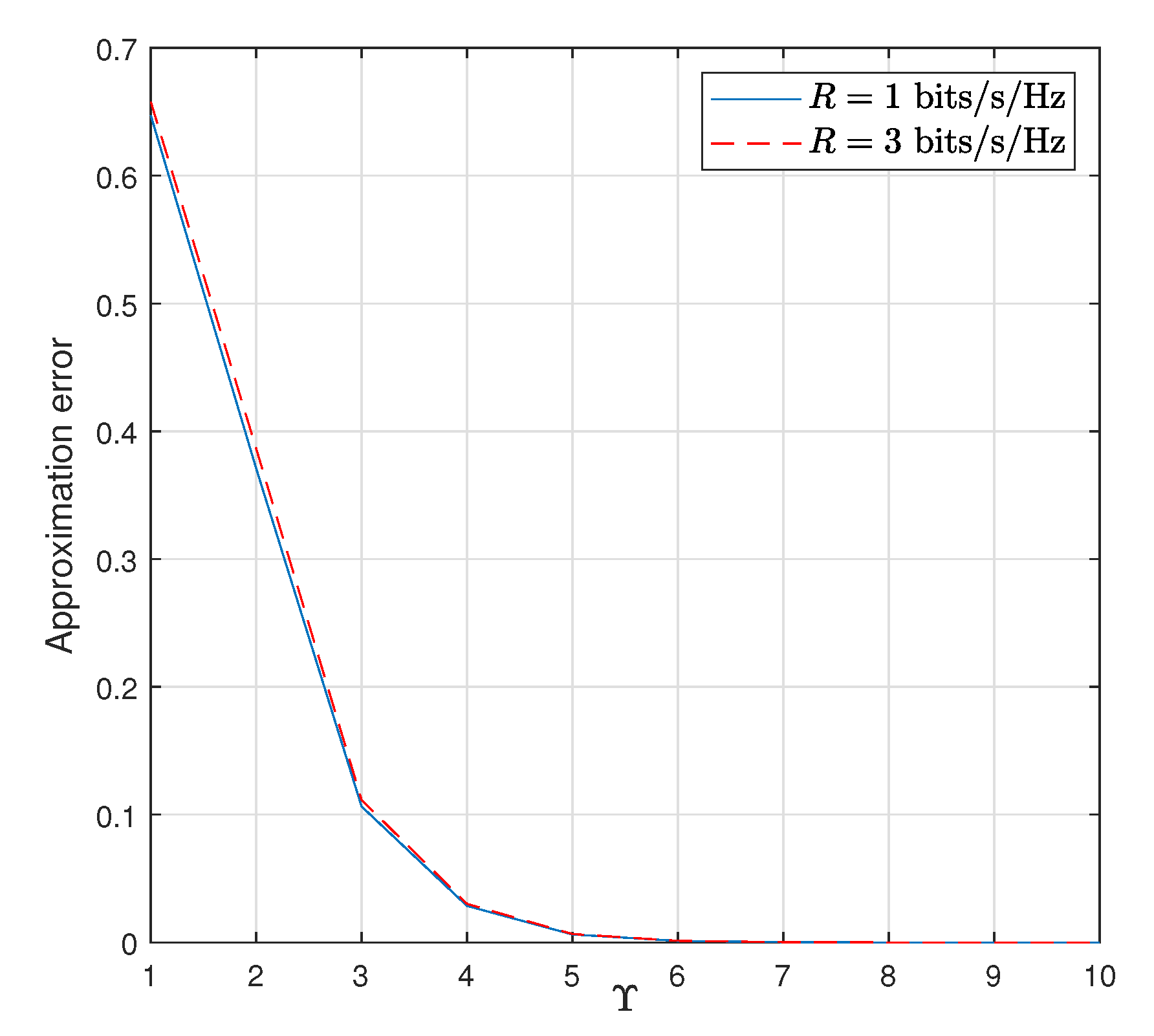
Figure 3 represents the relative approximation error of the throughput with respect to the parameter ${\rm Y}$. Specifically, we define

$$\begin{array}{c}\hfill \epsilon =\left|{\displaystyle \frac{\mathrm{analytical}\mathrm{value}-\mathrm{simulation}\mathrm{value}}{\mathrm{simulation}\mathrm{value}}}\right|\end{array}$$

(56)

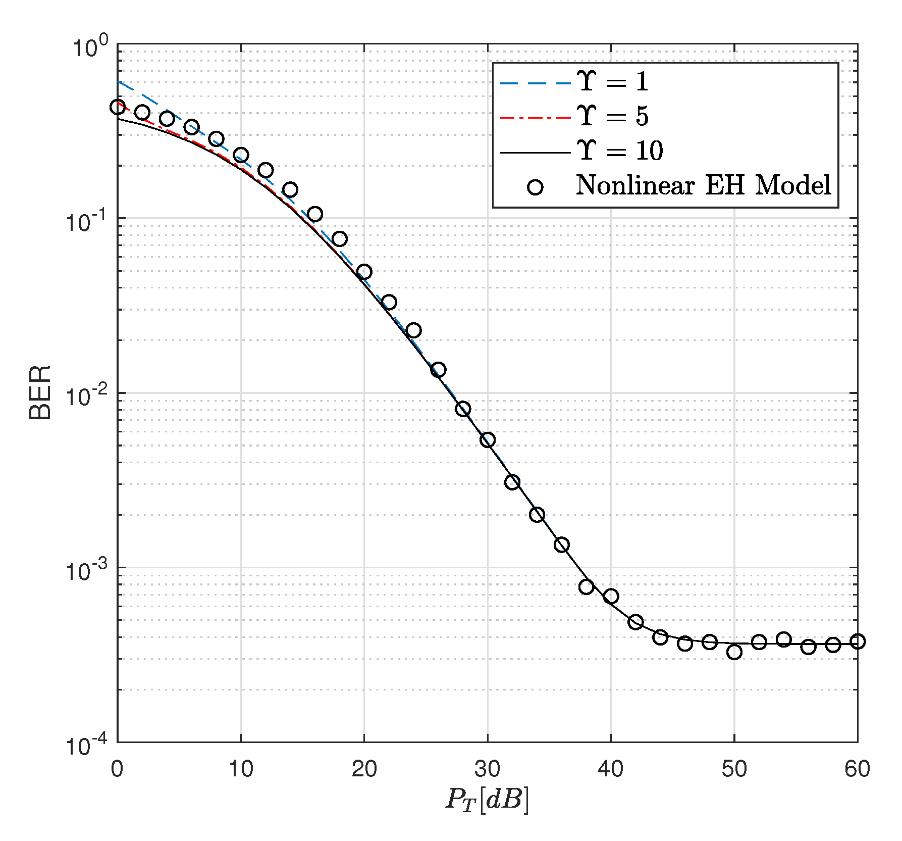
as the amount of relative error. Here the simulation value is obtained by the Monte Carlo method while the analytical value is calculated from (35). As seen from Figure 3, for both $R=1$ and $R=3$ bits/sec/Hz, by increasing the value of ${\rm Y}$, the error is decreased and tends to zero. Moreover, the results are sufficiently accurate when they are obtained for ${\rm Y}=7$, which provides an error value of $\epsilon =0.0002$. However, we guaranteed the results by taking ${\rm Y}=200$. In addition, the BER results are depicted in Figure 4 for different values of ${\rm Y}$ considering (15). From Figure 4, it is concluded that ${\rm Y}=10$ provides more accurate upper bound values compared to ${\rm Y}=1$.

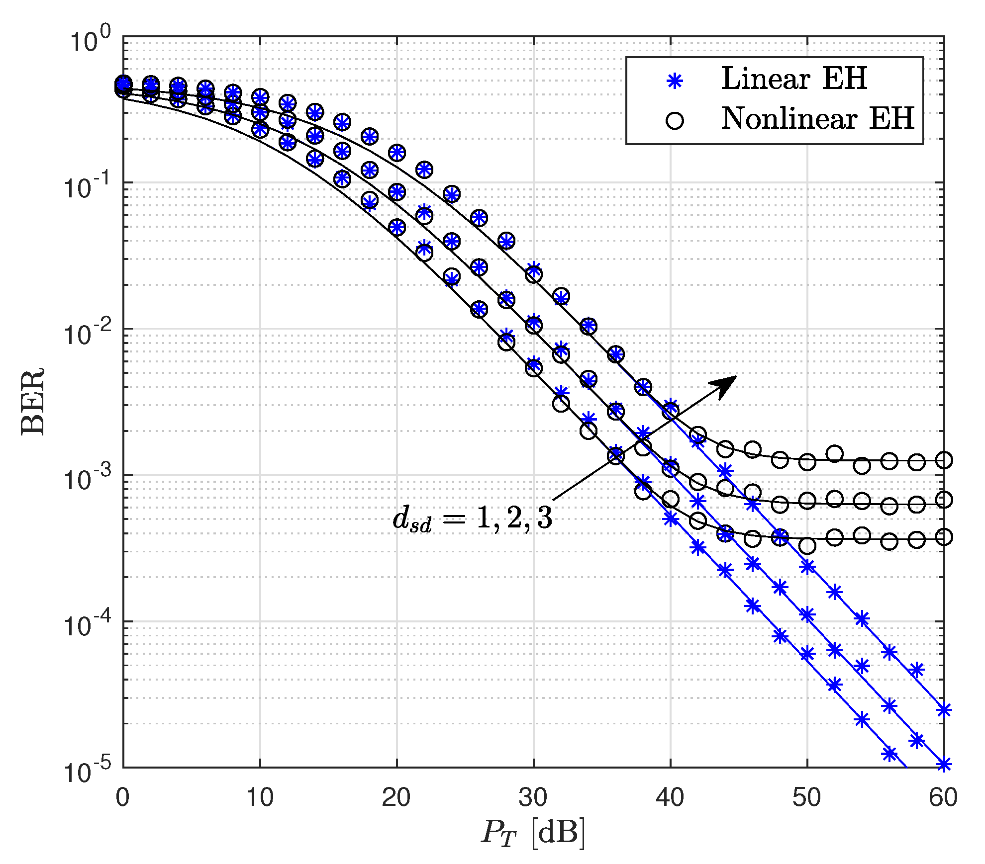
The BER performance of the proposed WP DH AF relaying system with respect to $P_T$ is presented in Figure 5. For $P_T$ values lower than 40 dB, the linear and non-linear models provide the same performance, while for $P_T$ higher than 40 dB, the BER performance for the non-linear EH model converges to the error floor, which verifies that the harvested power is higher than the threshold power. In other words, for higher SNR values, $P_s=P_r=P_{th}$. It is seen from Figure 5 that the linear EH model overestimates the system performance compared to the realistic results obtained for the non-linear EH model. Moreover, considering the linear EH model, approximately, 2 dB, and 6 dB SNR losses are obtained for the BER of ${10}^{-3}$ by increasing the value of $d_{sd}$ from 1 to 2 and 3, respectively.

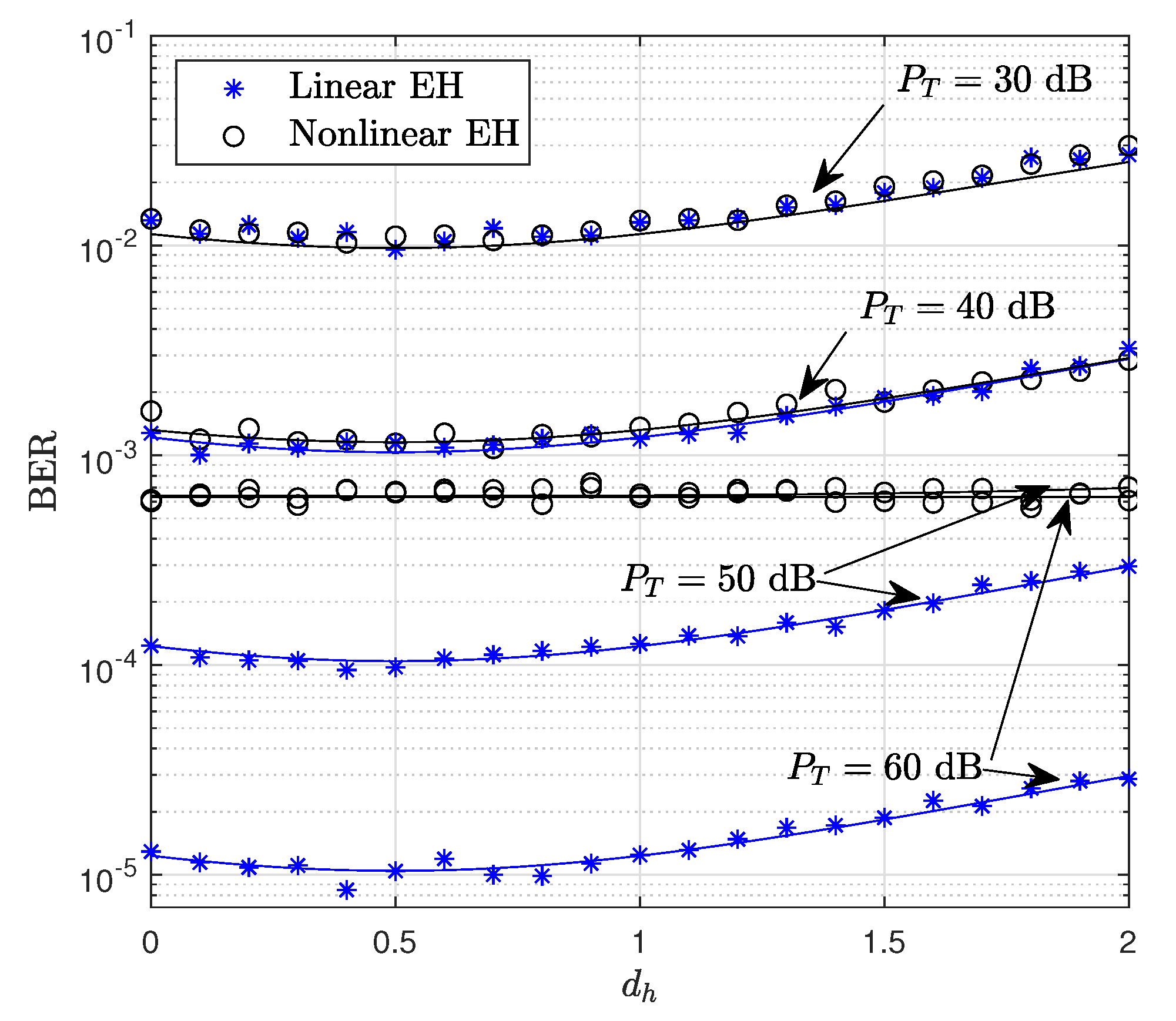
Figure 6 shows the BER performance versus $d_h$, where it is assumed that $d_{sd}=2$. It is seen from Figure 6 that the results provided for $P_T=30$ dB and $P_T=40$ dB are similar for both linear and non-linear EH models, since the threshold power in the non-linear EH model is assumed as $P_{th}=35$ dB, and the amount of harvested energy in both models is equal. However, for higher values of $P_T$, the linear EH model outperforms the non-linear EH where the amount of harvested power is saturated at $P_{th}=35$ dB, which weakens the system performance compared to the linear EH model. Please note that for $P_T=50$ dB and $P_T=60$ dB, the results provided for the non-linear EH model are approximately the same, since for higher input power of PB, $P_s$ and $P_r$ are limited by $P_{th}=35$ dB.

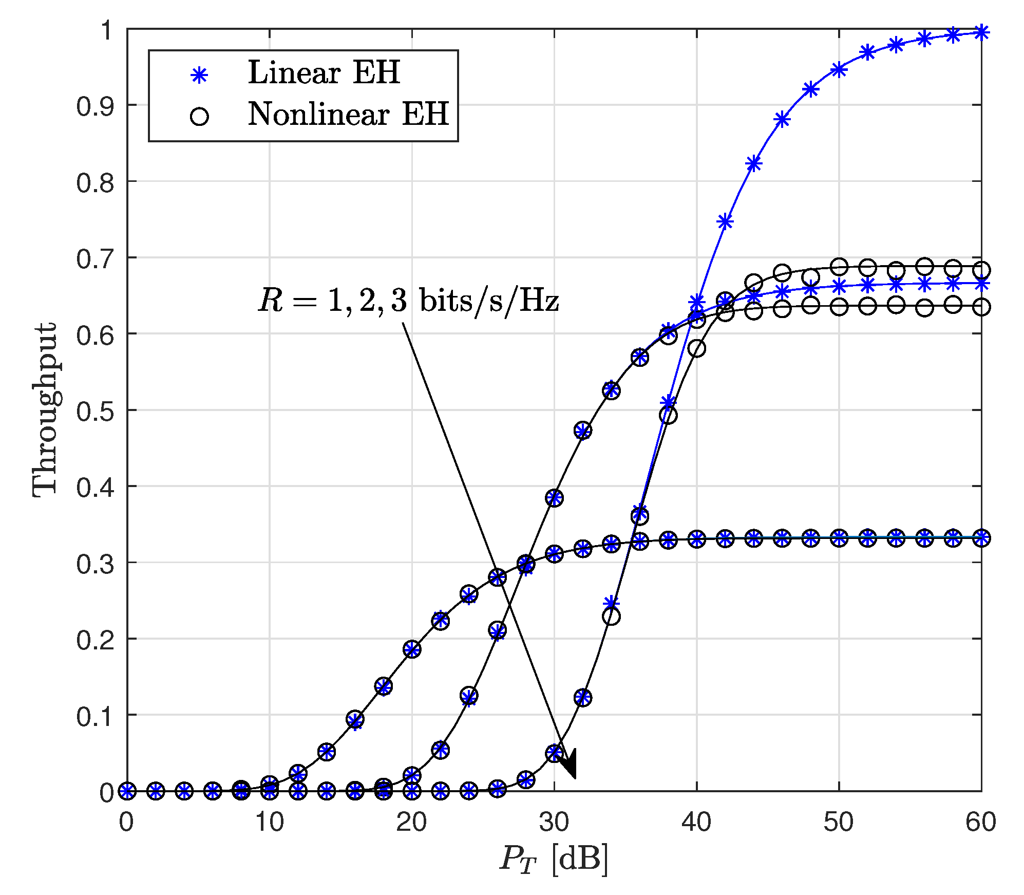
The throughput of the considered system versus $P_T$ for $d_{sd}=1$ is illustrated in Figure 7. It is shown that for a target rate value of $R=1$ bit/sec/Hz, the linear and non-linear EH models provide approximately the same performance, while for both $R=2$ and $R=3$, the linear EH model has higher throughput compared to the non-linear EH model. This is based on the fact that the linear EH model causes a misrepresentation of the system performance compared to the considered EH model since the amount of the harvested energy at both S and R nodes is miscalculated. Hence, this provides a misunderstanding of the design of the EH systems.

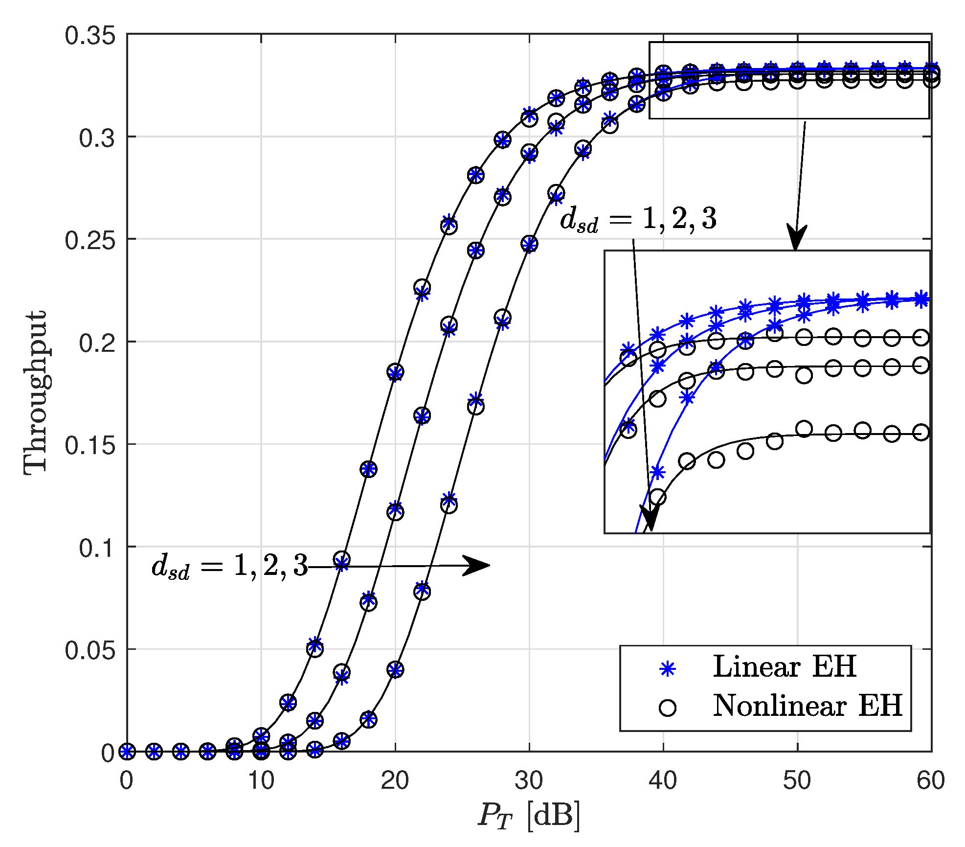
Figure 8 depicts the throughput with respect to $P_T$ for different values of $d_{sd}$. The target rate is fixed at $R=1$. The results reveal that, for the distances $d_{sd}=1,2,3$, the linear EH model provides performance approximately equivalent to that of the non-linear EH since the amount of harvested powers are approximately equal for both EH models. Moreover, in all cases, the throughput reaches its maximum value at $P_T=42$ dB.

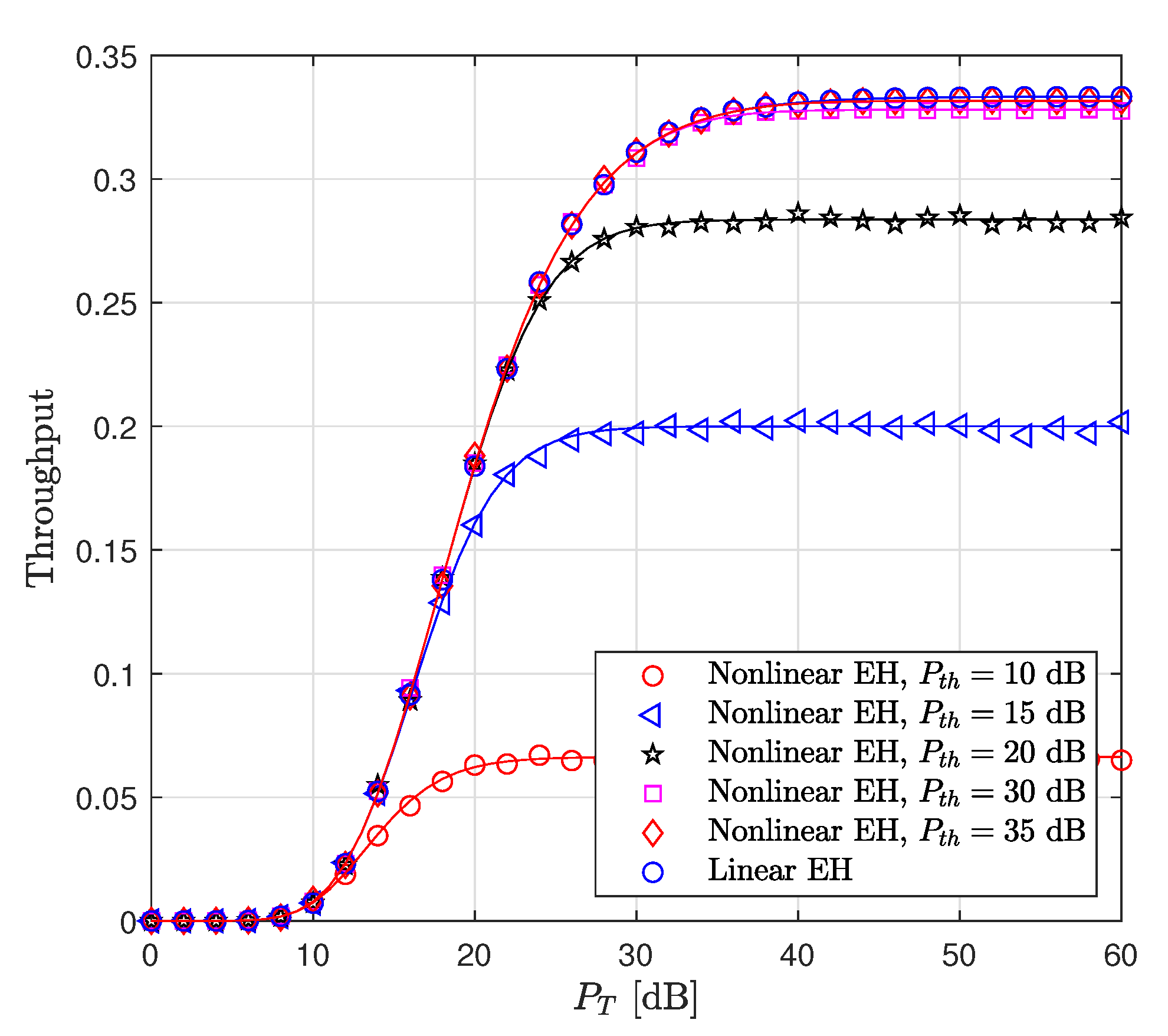
The throughput performance versus $P_T$ for different values of $P_{th}$ is shown in Figure 9. It is seen from Figure 9 that, by increasing $P_{th}$ from 10 dB to 35 dB, the throughput increases and reaches its maximum value for $P_{th}=35$ dB, which is approximately equivalent to the linear EH model throughput performance. In other words, a high level of threshold power in the non-linear EH model provides the same results as in the linear EH model since the amount of harvested power for both EH models is equal.

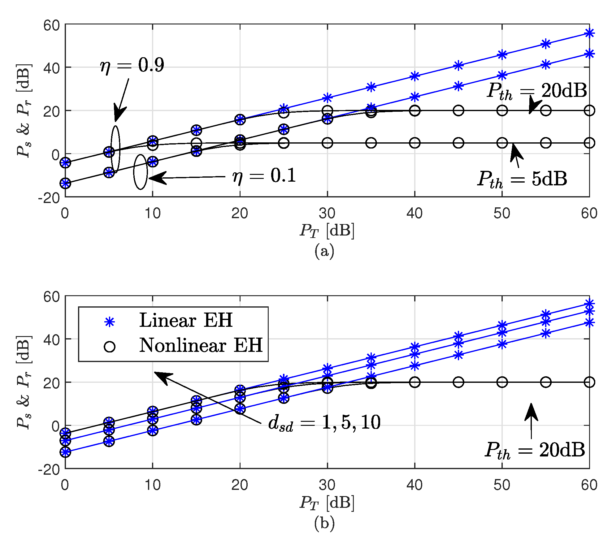
Figure 10 plots the source and relay harvested powers versus $P_T$. Please note that, from Appendix D, for an equal distance of S and R from PB, and for equal fading channel parameters, the harvested powers $P_s$ and $P_r$ are equal. The curves in Figure 10 are obtained using (A34) and (A35) for linear and non-linear EH models, respectively. As seen from Figure 10a,b, the distance ($d_{sd}$) and energy efficiency ($\eta$) have a significant effect on the amount of powers harvested at S and R. It is observed that, for high values of $P_T$, the average harvested power in the linear EH model is higher compared to the considered non-linear EH model, which is saturated to a predefined threshold value $P_{th}$. This high value is contrary to the amount of harvested energy in practical NL EH models, where it results in an overestimation of system performance.

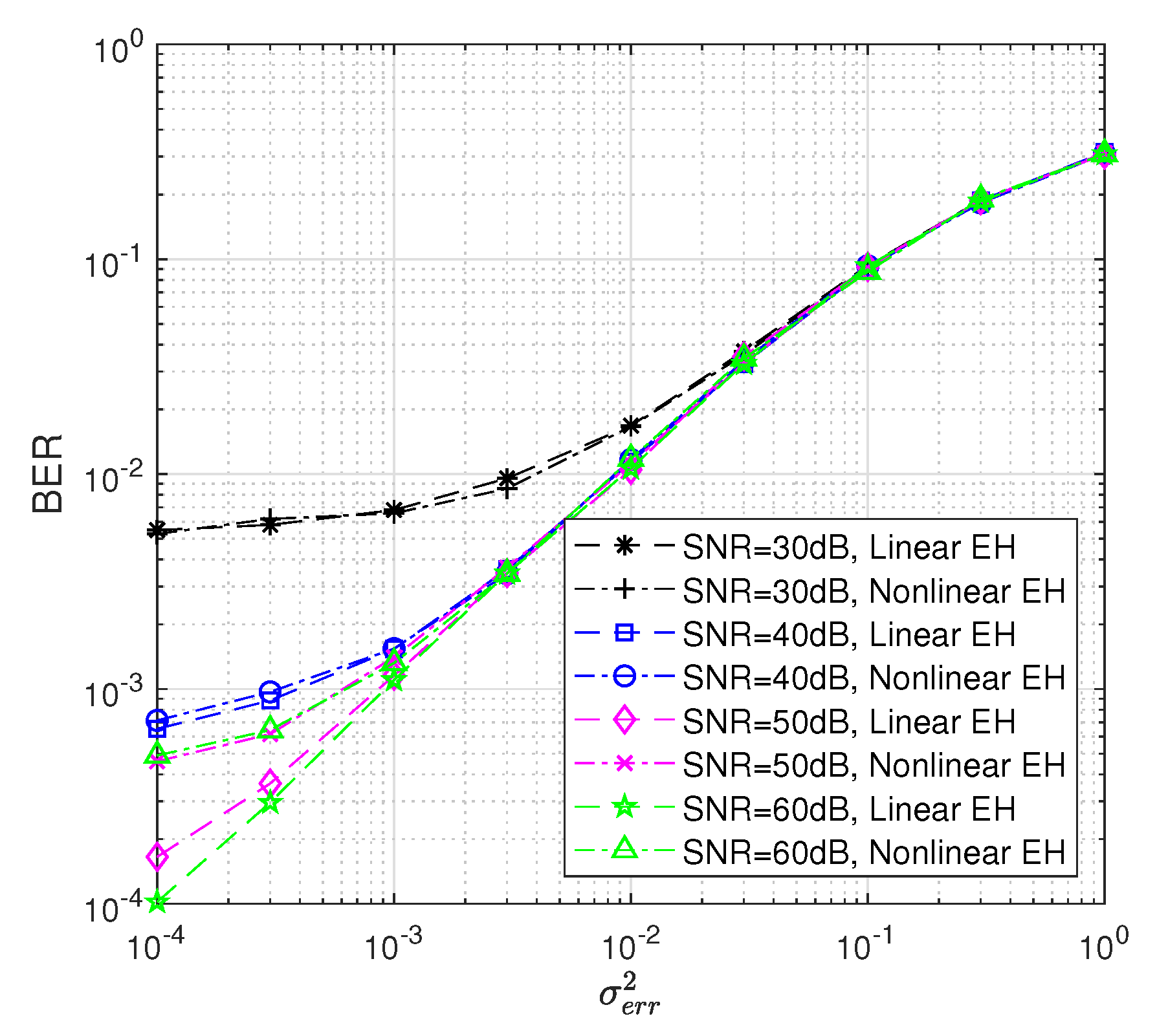
Figure 11 shows the BER performance versus channel estimation error power ${\sigma }_{err}^2$ for different SNR values. Both linear and non-linear EH results are obtained considering $P_{th}=35$ dB and $d_{sd}=1$. Moreover, we modeled the imperfect CSI case as $\widehat{g_1}=g_1+e$ and $\widehat{g_2}=g_2+e$, where e denotes the the channel estimation error with distribution $\mathcal{CN}\sim (0,{\sigma }_{err}^2)$, ${\sigma }_{err}^2$ denoting the power of the channel estimation error. It is shown that system performances get worse when the power of channel estimation error increases for both linear and non-linear EH models.

7. Conclusions

In this paper, a WP DH AF relaying system has been considered and a comprehensive performance analysis has been undertaken considering linear and non-linear EH models. In the studied system, S and R have been assumed to be battery-less, and that they harvest their power from a dedicated PB. For a comprehensive analysis, the results have been obtained considering the non-linear EH model together with the linear EH model which is mostly assumed in the literature. The BEP and throughput of the system for both linear and non-linear EH models have been analytically derived and compared with Monte Carlo simulation results, which verify our theoretical derivations. Moreover, results have been provided for different system parameters. It has been shown that the linear EH model misrepresents the system performance at high amounts of harvested energy and only provides reasonable results at low amounts of harvested energy. Hence, this causes an inaccurate understanding of the process of EH system design. However, the studied non-linear EH model provides a realistic result for the system performance, both at low and high harvested energy levels, which provides a comprehensive insight into the EH system architecture. We considered the case of a single antenna in all nodes in this paper. However, it is possible to have more antennas at the S, R, and D nodes and to analyze the improved system performance based on transmit antenna selection and maximum ratio combining. The analysis of these systems will be part of future work.

References

- Ding, Z.; Krikidis, I.; Sharif, B.; Poor, H.V. Wireless Information and Power Transfer in Cooperative Networks with Spatially Random Relays. IEEE Trans. Wirel. Commun. 2014, 13, 4440–4453. [Google Scholar] [CrossRef] [Green Version]
- Nasir, A.A.; Zhou, X.; Durrani, S.; Kennedy, R.A. Relaying Protocols for Wireless Energy Harvesting and Information Processing. IEEE Trans. Wirel. Commun. 2013, 12, 3622–3636. [Google Scholar] [CrossRef] [Green Version]
- Varshney, L.R. Transporting information and energy simultaneously. In Proceedings of the 2008 IEEE International Symposium on Information Theory, Toronto, ON, Canada, 6–11 July 2008; pp. 1612–1616. [Google Scholar] [CrossRef] [Green Version]
- Babaei, M.; Aygölü, Ü.; Basar, E. BER Analysis of Dual-Hop Relaying With Energy Harvesting in Nakagami-m Fading Channel. IEEE Trans. Wirel. Commun. 2018, 17, 4352–4361. [Google Scholar] [CrossRef]
- Zheng, L.; Zhai, C. Two-hop cognitive DF relaying with wireless power transfer in time and power domains. EURASIP J. Wirel. Commun. Netw. 2021, 2021, 182. [Google Scholar] [CrossRef]
- Mahmood, N.H.; Böcker, S.; Moerman, I.; López, O.A.; Munari, A.; Mikhaylov, K.; Clazzer, F.; Bartz, H.; Park, O.S.; Mercier, E.; et al. Machine type communications: Key drivers and enablers towards the 6G era. EURASIP J. Wirel. Commun. Netw. 2021, 2021, 134. [Google Scholar] [CrossRef]
- Munir, D.; Shah, S.T.; Choi, K.W.; Lee, T.J.; Chung, M.Y. Performance analysis of wireless-powered cognitive radio networks with ambient backscatter. EURASIP J. Wirel. Commun. Netw. 2019, 2019, 45. [Google Scholar] [CrossRef]
- Zhang, J.; Pan, G. Outage Analysis of Wireless-Powered Relaying MIMO Systems with Non-Linear Energy Harvesters and Imperfect CSI. IEEE Access 2016, 4, 7046–7053. [Google Scholar] [CrossRef]
- Xu, X.; Özçelikkale, A.; McKelvey, T.; Viberg, M. Simultaneous information and power transfer under a non-linear RF energy harvesting model. In Proceedings of the 2017 IEEE International Conference on Communications Workshops (ICC Workshops), Paris, France, 21–25 May 2017; pp. 179–184. [Google Scholar] [CrossRef] [Green Version]
- Chen, Y.; Zhao, N.; Alouini, M. Wireless Energy Harvesting Using Signals From Multiple Fading Channels. IEEE Trans. Commun. 2017, 65, 5027–5039. [Google Scholar] [CrossRef] [Green Version]
- Dong, Y.; Hossain, M.J.; Cheng, J. Performance of Wireless Powered Amplify and Forward Relaying over Nakagami-m Fading Channels With Nonlinear Energy Harvester. IEEE Commun. Lett. 2016, 20, 672–675. [Google Scholar] [CrossRef]
- Chen, Y.; Sabnis, K.T.; Abd-Alhameed, R.A. New Formula for Conversion Efficiency of RF EH and Its Wireless Applications. IEEE Trans. Veh. Technol. 2016, 65, 9410–9414. [Google Scholar] [CrossRef] [Green Version]
- Boshkovska, E.; Ng, D.W.K.; Zlatanov, N.; Schober, R. Practical Non-Linear Energy Harvesting Model and Resource Allocation for SWIPT Systems. IEEE Commun. Lett. 2015, 19, 2082–2085. [Google Scholar] [CrossRef] [Green Version]
- Babaei, M.; Aygölü, Ü.; Durak-Ata, L. Performance of Selective Decode-and-Forward SWIPT Network in Nakagami-m Fading Channel. In Proceedings of the 2018 26th Telecommunications Forum (TELFOR), Belgrade, Serbia, 20–21 November 2018; pp. 1–4. [Google Scholar] [CrossRef]
- Wang, J.; Wang, G.; Li, B.; Yang, H.; Hu, Y.; Schmeink, A. Massive MIMO Two-Way Relaying Systems with SWIPT in IoT Networks. IEEE Internet Things J. 2021, 8, 15126–15139. [Google Scholar] [CrossRef]
- Sahu, H.K.; Padhan, A.K.; Sahu, P.R. Smart Devices Performance with SSK-BPSK Modulation and Energy Harvesting in Smart Cities. IEEE Commun. Lett. 2021, 25, 637–640. [Google Scholar] [CrossRef]
- Agrawal, K.; Prakriya, S.; Flanagan, M.F. Optimization of SWIPT with Battery-Assisted Energy Harvesting Full-Duplex Relays. IEEE Trans. Green Commun. Netw. 2021, 5, 243–260. [Google Scholar] [CrossRef]
- Lu, W.; Si, P.; Huang, G.; Han, H.; Qian, L.; Zhao, N.; Gong, Y. SWIPT Cooperative Spectrum Sharing for 6G-Enabled Cognitive IoT Network. IEEE Internet Things J. 2021, 8, 15070–15080. [Google Scholar] [CrossRef]
- Le, Q.N.; Yadav, A.; Nguyen, N.P.; Dobre, O.A.; Zhao, R. Full-Duplex Non-Orthogonal Multiple Access Cooperative Overlay Spectrum-Sharing Networks with SWIPT. IEEE Trans. Green Commun. Netw. 2021, 5, 322–334. [Google Scholar] [CrossRef]
- Li, X.; Wang, Q.; Liu, M.; Li, J.; Peng, H.; Piran, J.; Li, L. Cooperative Wireless-Powered NOMA Relaying for B5G IoT Networks with Hardware Impairments and Channel Estimation Errors. IEEE Internet Things J. 2021, 8, 5453–5467. [Google Scholar] [CrossRef]
- Ge, L.; Chen, G.; Zhang, Y.; Tang, J.; Wang, J.; Chambers, J.A. Performance Analysis for Multihop Cognitive Radio Networks With Energy Harvesting by Using Stochastic Geometry. IEEE Internet Things J. 2020, 7, 1154–1163. [Google Scholar] [CrossRef]
- Chen, G.; Xiao, P.; Kelly, J.R.; Li, B.; Tafazolli, R. Full-Duplex Wireless-Powered Relay in Two Way Cooperative Networks. IEEE Access 2017, 5, 1548–1558. [Google Scholar] [CrossRef] [Green Version]
- Zhang, Q.; Wang, Z.; Zhang, P.; Zhang, H.; Wan, X.; Fan, Z. Sum energy maximization for UAV-enabled wireless power transfer networks with non-linear energy harvesting model. In Proceedings of the 2020 IEEE 4th Information Technology, Networking, Electronic and Automation Control Conference (ITNEC), Chongqing, China, 12–14 June 2020; Volume 1, pp. 1417–1420. [Google Scholar] [CrossRef]
- Parvez, S.; Kumar, D.; Bhatia, V. On Performance of SWIPT Enabled Two-Way Relay System with Non-Linear Power Amplifier. In Proceedings of the 2020 National Conference on Communications (NCC), Kharagpur, India, 21–23 February 2020; pp. 1–6. [Google Scholar] [CrossRef]
- Huang, Y.; Duong, T.Q.; Wang, J.; Zhang, P. Performance of Multi-Antenna Wireless-Powered Communications with Nonlinear Energy Harvester. In Proceedings of the 2017 IEEE 86th Vehicular Technology Conference (VTC-Fall), Toronto, ON, Canada, 24–27 September 2017; pp. 1–6. [Google Scholar] [CrossRef]
- Feng, Y.; Wen, M.; Ji, F.; Leung, V.C.M. Performance Analysis for BDPSK Modulated SWIPT Cooperative Systems with Nonlinear Energy Harvesting Model. IEEE Access 2018, 6, 42373–42383. [Google Scholar] [CrossRef]
- Wang, K.; Li, Y.; Ye, Y.; Zhang, H. Dynamic Power Splitting Schemes for Non-Linear EH Relaying Networks: Perfect and Imperfect CSI. In Proceedings of the 2017 IEEE 86th Vehicular Technology Conference (VTC-Fall), Toronto, ON, Canada, 24–27 September 2017; pp. 1–5. [Google Scholar] [CrossRef]
- Xu, K.; Shen, Z.; Zhang, M.; Wang, Y.; Xia, X.; Xie, W.; Zhang, D. Beam-Domain SWIPT for mMIMO System With Nonlinear Energy Harvesting Legitimate Terminals and a Non-Cooperative Terminal. IEEE Trans. Green Commun. Netw. 2019, 3, 703–720. [Google Scholar] [CrossRef]
- Wei, Z.; Sun, S.; Zhu, X.; In Kim, D.; Ng, D.W.K. Resource Allocation for Wireless-Powered Full-Duplex Relaying Systems with Nonlinear Energy Harvesting Efficiency. IEEE Trans. Veh. Technol. 2019, 68, 12079–12093. [Google Scholar] [CrossRef]
- Babaei, M.; Aygölü, Ü.; Başaran, M.; Durak-Ata, L. BER Performance of Full-Duplex Cognitive Radio Network with Nonlinear Energy Harvesting. IEEE Trans. Green Commun. Netw. 2020, 4, 448–460. [Google Scholar] [CrossRef]
- Hakimi, A.; Mohammadi, M.; Mobini, Z.; Ding, Z. Full-Duplex Non-Orthogonal Multiple Access Cooperative Spectrum-Sharing Networks with Non-Linear Energy Harvesting. IEEE Trans. Veh. Technol. 2020, 69, 10925–10936. [Google Scholar] [CrossRef]
- Liu, Y.; Ye, Y.; Ding, H.; Gao, F.; Yang, H. Outage Performance Analysis for SWIPT-Based Incremental Cooperative NOMA Networks with Non-Linear Harvester. IEEE Commun. Lett. 2020, 24, 287–291. [Google Scholar] [CrossRef]
- Solanki, S.; Upadhyay, P.K.; da Costa, D.B.; Ding, H.; Moualeu, J.M. Non-Linear Energy Harvesting Based Cooperative Spectrum Sharing Networks. In Proceedings of the 2019 16th International Symposium on Wireless Communication Systems (ISWCS), Oulu, Finland, 27–30 August 2019; pp. 566–570. [Google Scholar] [CrossRef]
- Zhang, Y.; Jiang, R.; Gao, S.; Xiong, K.; Zhou, L.; Liu, T. Outage Performance of Two-hop Networks with Multiple SWIPT Relays under Nonlinear EH Model. In Proceedings of the 2018 14th IEEE International Conference on Signal Processing (ICSP), Beijing, China, 12–16 August 2018; pp. 752–757. [Google Scholar] [CrossRef]
- Nguyen, T.L.N.; Shin, Y. Outage Probability Analysis for SWIPT Systems with Nonlinear Energy Harvesting Model. In Proceedings of the 2019 International Conference on Information and Communication Technology Convergence (ICTC), Jeju, Korea, 16–18 October 2019; pp. 196–199. [Google Scholar] [CrossRef]
- Ma, G.; Xu, J.; Zeng, Y.; Moghadam, M.R.V. A Generic Receiver Architecture for MIMO Wireless Power Transfer with Nonlinear Energy Harvesting. IEEE Signal Process. Lett. 2019, 26, 312–316. [Google Scholar] [CrossRef] [Green Version]
- Kang, J.; Chun, C.; Kim, I.; Kim, D.I. Dynamic Power Splitting for SWIPT With Nonlinear Energy Harvesting in Ergodic Fading Channel. IEEE Internet Things J. 2020, 7, 5648–5665. [Google Scholar] [CrossRef] [Green Version]
- Nguyen, T.T.; Nguyen, V.D.; Pham, Q.V.; Lee, J.H.; Kim, Y.H. Resource Allocation for AF Relaying Wireless-Powered Networks with Nonlinear Energy Harvester. IEEE Commun. Lett. 2021, 25, 229–233. [Google Scholar] [CrossRef]
- Yang, H.; Ye, Y.; Chu, X.; Dong, M. Resource and Power Allocation in SWIPT-Enabled Device-to-Device Communications Based on a Nonlinear Energy Harvesting Model. IEEE Internet Things J. 2020, 7, 10813–10825. [Google Scholar] [CrossRef]
- Shi, L.; Ye, Y.; Chu, X.; Lu, G. Computation Bits Maximization in a Backscatter Assisted Wirelessly Powered MEC Network. IEEE Commun. Lett. 2021, 25, 528–532. [Google Scholar] [CrossRef]
- Illi, E.; El Bouanani, F.; Sofotasios, P.C.; Muhaidat, S.; da Costa, D.B.; Ayoub, F.; Al-Fuqaha, A. Analysis of Asymmetric Dual-Hop Energy Harvesting-Based Wireless Communication Systems in Mixed Fading Environments. IEEE Trans. Green Commun. Netw. 2021, 5, 261–277. [Google Scholar] [CrossRef]
- Zhu, Z.; Wang, N.; Hao, W.; Wang, Z.; Lee, I. Robust Beamforming Designs in Secure MIMO SWIPT IoT Networks with a Non-Linear Channel Model. IEEE Internet Things J. 2021, 1–6. [Google Scholar] [CrossRef]
- Raut, P.; Singh, K.; Li, C.P.; Alouini, M.S.; Huang, W.J. Nonlinear EH-Based UAV-Assisted FD IoT Networks: Infinite and Finite Blocklength Analysis. IEEE Internet Things J. 2021, 8, 17655–17668. [Google Scholar] [CrossRef]
- Wang, S.; Xia, M.; Huang, K.; Wu, Y.C. Wirelessly Powered Two-Way Communication With Nonlinear Energy Harvesting Model: Rate Regions Under Fixed and Mobile Relay. IEEE Trans. Wirel. Commun. 2017, 16, 8190–8204. [Google Scholar] [CrossRef]
- Kang, J.; Kim, I.; Kim, D.I. Joint Tx Power Allocation and Rx Power Splitting for SWIPT System With Multiple Nonlinear Energy Harvesting Circuits. IEEE Wirel. Commun. Lett. 2019, 8, 53–56. [Google Scholar] [CrossRef] [Green Version]
- Li, Z.; Chen, H.; Li, Y.; Vucetic, B. Wireless Energy Harvesting Cooperative Communications with Direct Link and Energy Accumulation. arXiv 2016, arXiv:1608.04165. [Google Scholar]
- Zhong, C.; Chen, X.; Zhang, Z.; Karagiannidis, G.K. Wireless-Powered Communications: Performance Analysis and Optimization. IEEE Trans. Commun. 2015, 63, 5178–5190. [Google Scholar] [CrossRef] [Green Version]
- Gu, Y.; Chen, H.; Li, Y.; Liang, Y.; Vucetic, B. Distributed Multi-Relay Selection in Accumulate-Then-Forward Energy Harvesting Relay Networks. IEEE Trans. Green Commun. Netw. 2018, 2, 74–86. [Google Scholar] [CrossRef] [Green Version]
- Zhang, R.; Chen, H.; Yeoh, P.L.; Li, Y.; Vucetic, B. Full-duplex cooperative cognitive radio networks with wireless energy harvesting. In Proceedings of the 2017 IEEE International Conference on Communications (ICC), Paris, France, 21–25 May 2017; pp. 1–6. [Google Scholar] [CrossRef] [Green Version]
- Gradshteyn, I.S.; Ryzhik, I.M.; Romer, R.H. Tables of Integrals, Series, and Products; Academic Press: Cambridge, MA, USA, 2014. [Google Scholar]
- Abramowitz, M. Handbook of Mathematical Functions, with Formulas, Graphs, and Mathematical Tables; Dover Publications, Inc.: Mineola, NY, USA, 1974. [Google Scholar]
- Wolfram. The Wolfram Functions Site. 2001. Available online: http://functions.wolfram.com (accessed on 25 April 2022).
- Le, T.; Mayaram, K.; Fiez, T. Efficient Far-Field Radio Frequency Energy Harvesting for Passively Powered Sensor Networks. IEEE J. Solid-State Circuits 2008, 43, 1287–1302. [Google Scholar] [CrossRef]
- Papoulis, A.; Pillai, S. Probability, Random Variables, and Stochastic Processes; McGraw-Hill: Boston, MA, USA, 2002. [Google Scholar]
- Simon, M.; Alouini, M. Digital Communication over Fading Channels; Wiley McGraw-Hill: New York, NY, USA, 2005. [Google Scholar]
- Adamchik, V.S.; Marichev, O.I. The Algorithm for Calculating Integrals of Hypergeometric Type Functions and Its Realization in REDUCE System. In Proceedings of the International Symposium on Symbolic and Algebraic Computation (ISSAC), Tokyo, Japan, 20–24 August 1990; pp. 212–224. [Google Scholar] [CrossRef]
- Meyr, H.; Moeneclaey, M.; Fechtel, S. Digital Communication Receivers: Synchronization, Channel Estimation, and Signal Processing; John Wiley & Sons, Inc.: New York, NY, USA, 1997. [Google Scholar]
Figure 1.
Wireless-powered DH AF relaying system model where S and R harvest their energy from a dedicated PB. S and R use their harvested power for data transmission.
Figure 2.
Transmission time frame of the considered wireless-powered system. The transmission frame is assumed to be equally-partitioned into three time slots for EH and information processing (IP).
Figure 3.
Relative approximation error versus parameter of the WP DH AF relaying system for dB, and dB.
Figure 4.
BER performance of the WP DH AF relaying system versus dB for dB.
Figure 5.
BER performance of the WP DH AF relaying system versus dB where dB.
Figure 6.
BER performance of the WP DH AF relaying system versus (, dB).
Figure 7.
Throughput performance of the WP DH AF relaying system versus (, dB).
Figure 8.
Throughput performance of the WP DH AF relaying system versus ( bits/s/Hz, dB).
Figure 9.
Throughput performance of the WP DH AF relaying system versus ( bits/s/Hz, ).
Figure 10.
and of the WP DH AF relaying system (a) , (b) .
Figure 11.
BER performance of the WP DH AF relaying system versus dB where = 35 dB, .