
Enhanced Ambient Sensing Environment—A New Method for Calibrating Low-Cost Gas Sensors

 , ,
, ,  , , and
Abstract
:
1. Introduction
2. Materials and Methods
2.1. Sensor Nodes
2.1.1. Gen 2 MOx Nodes
2.1.2. Gen 5 EC Nodes
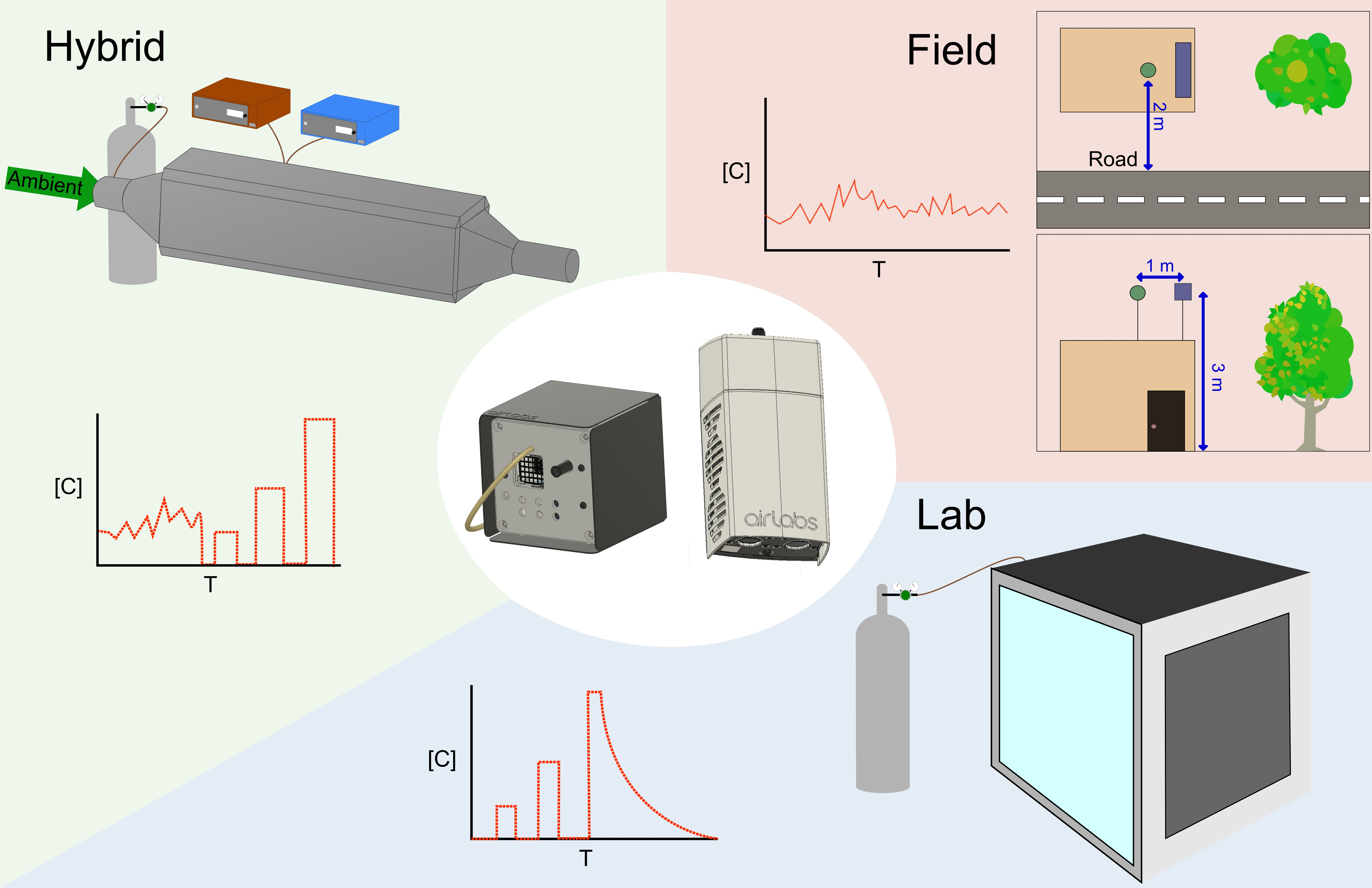
2.2. Calibration Method Overview
2.2.1. MOx Laboratory Calibration Protocol
2.2.2. MOx EASE Calibration Protocol
2.2.3. MOx Field Calibration Protocol
2.2.4. MOx Calibration Models
2.2.5. EC Laboratory Calibration Protocol
2.2.6. EC EASE Calibration Protocol
2.2.7. EC Field Calibration Protocol
2.2.8. EC Calibration Models
3. Results and Discussion
3.1. Mox Node Results
3.2. EC Node Results
3.3. Node Comparison
4. Conclusions
Author Contributions
Funding
Data Availability Statement
Acknowledgments
Conflicts of Interest
Abbreviations
| AE | Auxiliary Electrode |
| AQ | Air Quality |
| EASE | Enhanced ambient Sensing Environment |
| EC | ElectroChemical |
| HCAB | H. C. Andersens Boulevard |
| LCS | Low-Cost Sensor |
| LR | Linear Regression |
| MAE | Mean Absolute Error |
| MBE | Mean Bias Error |
| MFC | Mass Flow Controller |
| ML | Machine Learning |
| MLR | Multivariate Linear Regression |
| MOx | Metal-Oxide |
| PCB | Printed Circuit Board |
| RH | Relative Humidity |
| RMSE | Root Mean Square Error |
| T | Temperature |
| TCO | Temperature Cycling Operation |
| WE | Working Electrode |
Appendix A. Equipment Tests and Training Parameters
Appendix A.1. EASE


| Node | NO2-B43F Cell Serial | WE Zero Current/nA | AE Zero Current/nA | Sensitivity/ (nA ppm−1) |
|---|---|---|---|---|
| ANG500012 | 202750622 | 32.16 | 18.29 | −386.68 |
| ANG500149 | 202750349 | 19.86 | 2.84 | −338.6 |
| ANG500151 | 202750350 | 25.54 | 18.60 | −348.85 |
| ANG500174 | 202750153 | 30.58 | 11.35 | −400.24 |
| ANG500194 | 202750122 | 30.90 | 8.51 | −380.38 |
| ANG500208 | 202750105 | 31.21 | 12.30 | −412.38 |
| ANG500218 | 202750639 | 33.73 | 18.92 | −379.75 |
| ANG500219 | 202750638 | 33.42 | 21.44 | −384.32 |
| ANG500224 | 202055609 | 9.46 | 9.14 | −341.13 |
| ANG500225 | 202055604 | 25.22 | 17.66 | −319.37 |
| ANG500245 | 202240647 | 52.97 | 20.49 | −393.62 |
| ANG500252 | 202750601 | 24.91 | 17.34 | −355.63 |
| ANG500254 | 202750119 | 31.84 | 14.19 | −374.39 |
| ANG500255 | 202750110 | 35.63 | 15.76 | −368.87 |
| ANG500259 | 202750112 | 35.94 | 10.72 | −382.58 |
| Node | OX-B431 Cell Serial | WE Zero Current/nA | AE Zero Current/nA | Sensitivity/ nA ppm−1 |
|---|---|---|---|---|
| ANG500012 | 204050221 | 25.22 | 9.77 | −656.87 |
| ANG500149 | 204071554 | 37.20 | 24.59 | −548.26 |
| ANG500151 | 204071553 | 39.09 | 21.12 | −586.25 |
| ANG500174 | 204070150 | 47.29 | 17.66 | −480.64 |
| ANG500194 | 204751304 | −29.01 | 11.67 | −599.18 |
| ANG500208 | 204070439 | 34.36 | 11.98 | −543.37 |
| ANG500218 | 204070440 | 33.42 | 7.25 | −585.94 |
| ANG500219 | 204070441 | 44.45 | 17.97 | −489.46 |
| ANG500224 | 204070407 | 20.49 | 14.19 | −627.87 |
| ANG500225 | 204070406 | 37.52 | 10.72 | −570.02 |
| ANG500245 | 204851926 | 33.73 | 16.71 | −584.20 |
| ANG500252 | 204851922 | 39.41 | 20.18 | −613.37 |
| ANG500254 | 204851921 | 43.51 | 19.86 | −613.05 |
| ANG500255 | 204851916 | 36.89 | 17.34 | −626.76 |
| ANG500259 | 204851918 | 35.63 | 19.86 | −559.77 |
| Node | Offset Applied NO2/ppb | Offset Applied O3/ppb |
|---|---|---|
| ANG500012 | 24.80 | 52.20 |
| ANG500149 | 55.28 | 52.50 |
| ANG500151 | 58.55 | −62.56 |
| ANG500174 | 69.03 | −11.60 |
| ANG500194 | 37.55 | 43.46 |
| ANG500208 | 76.79 | −55.55 |
| ANG500218 | −21.66 | 46.76 |
| ANG500219 | 44.61 | −127.34 |
| ANG500224 | −20.53 | −10.62 |
| ANG500225 | 36.25 | −90.69 |
| ANG500245 | −7.93 | 122.58 |
| ANG500252 | 18.78 | 125.58 |
| ANG500254 | 45.48 | −7.23 |
| ANG500255 | 105.74 | −89.34 |
| ANG500259 | 101.61 | −175.24 |
| Max | 105.74 | 125.58 |
| Min | −21.66 | −175.24 |
| Difference | 127.41 | 300.82 |
| Node | Field | EASE | Laboratory |
|---|---|---|---|
| MOx | 22nd December 2020 : 3rd February 2021 | * 21st February 2021 : 26th February 2021 | 12th March 2021 : 15th March 2021 |
| EC | 9th December 2021 : 23rd December 2021 | ** 1st September 2021 : 5th October 2021 | Prior to dispatch (then sealed) |
| Pollutant | Method | Slope | Intercept/ppb | RMSE/ppb | MBE/ppb | MAE/ppb | |
|---|---|---|---|---|---|---|---|
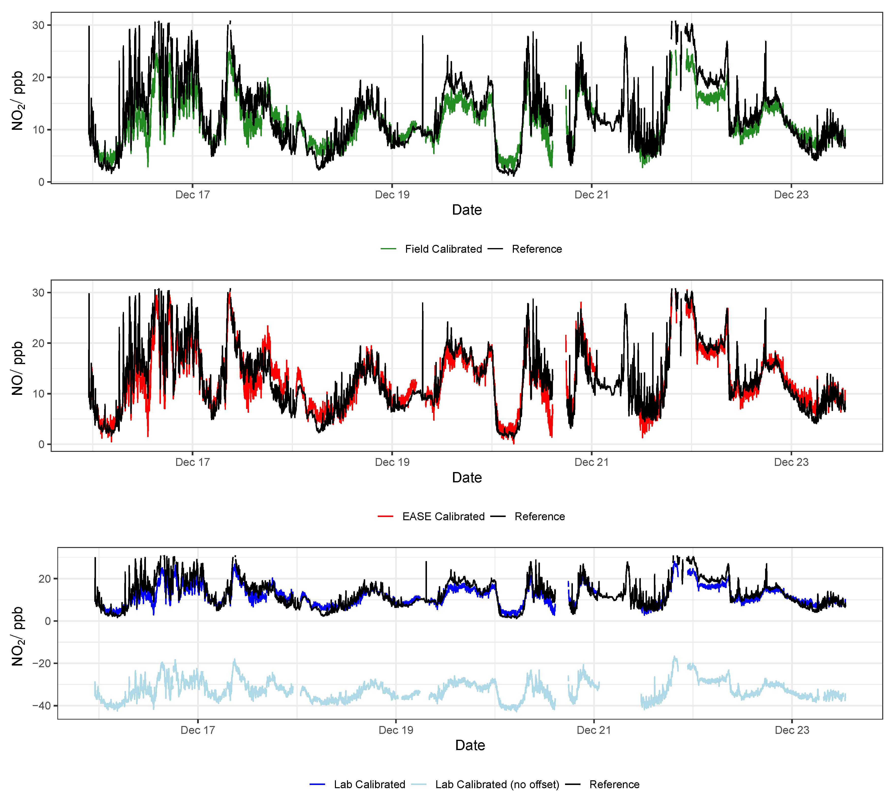
| NO2 | Laboratory | 0.90 (0.047) | 1.0 (0.0) | 0.0 (0.0) | 9.9 (2.7) | 0.0 (0.0) | 6.6 (1.7) |
| EASE | 0.96 (0.014) | 1.0 (0.0) | 0.0 (0.0) | 3.7 (0.67) | 0.0 (0.0) | 2.6 (0.32) | |
| Field | 0.92 (0.040) | 1.0 (0.0) | 0.0 (0.0) | 3.6 (0.86) | 0.0 (0.0) | 2.6 (0.67) | |
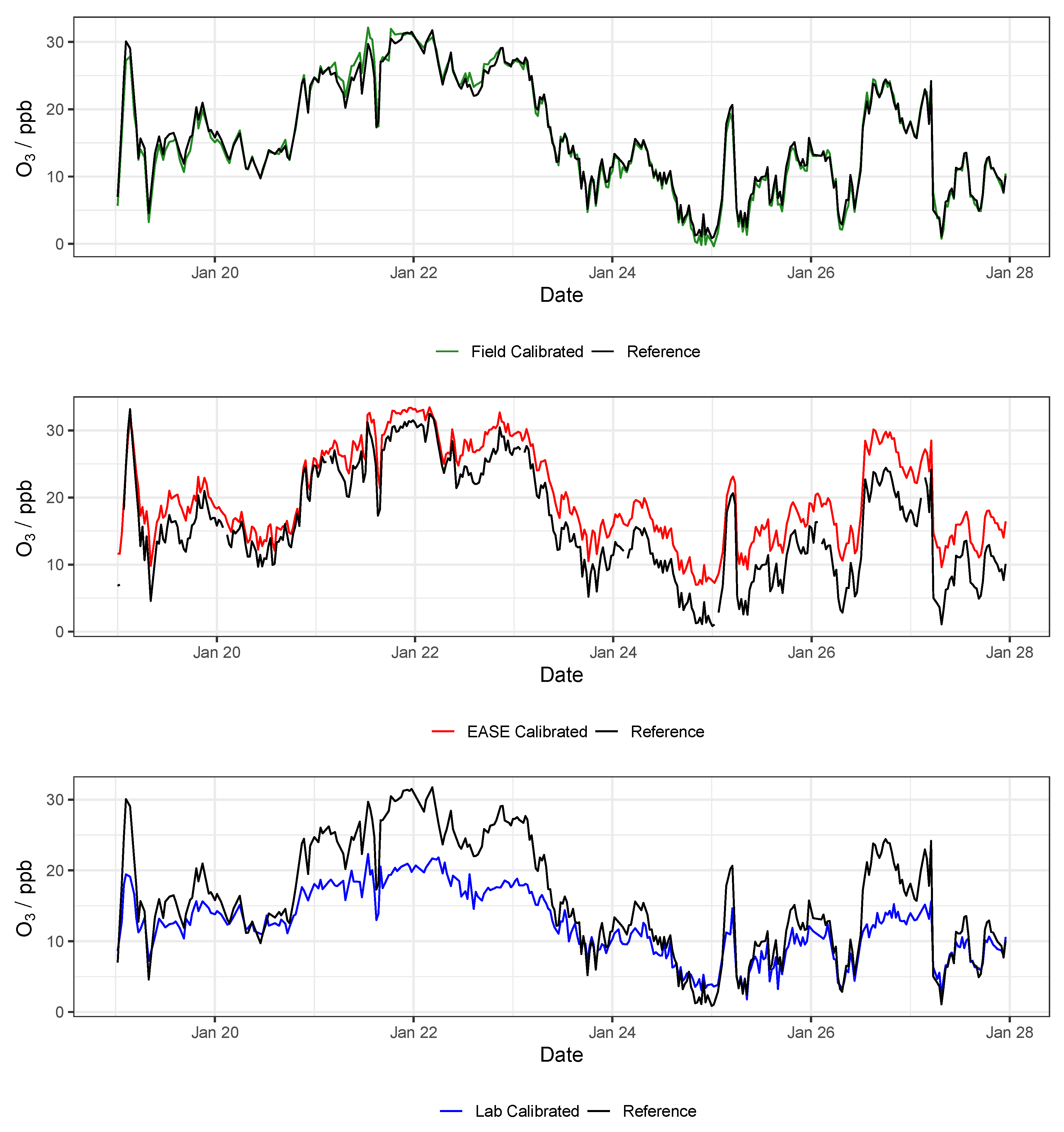
| O3 | Laboratory | 0.99 (0.011) | 1.0 (0.0) | 0.0 (0.0) | 3.3 (1.2) | 0.0 (0.0) | 2.2 (0.86) |
| EASE | 0.97 (0.013) | 1.0 (0.0) | 0.0 (0.0) | 2.7 (0.72) | 0.0 (0.0) | 1.5 (0.51) | |
| Field | 0.96 (0.040) | 1.0 (0.0) | 0.0 (0.0) | 1.2 (0.71) | 0.0 (0.0) | 0.90 (0.57) |
| Pollutant | Method | Slope | Intercept/ppb | RMSE/ppb | MBE/ppb | MAE/ppb | |
|---|---|---|---|---|---|---|---|
| NO2 | EASE | 0.94 (0.040) | 1.0 (0.0) | 0.0 (0.0) | 5.2 (1.6) | 0.0 (0.0) | 4.0 (1.4) |
| Field | 0.49 (0.082) | 1.0 (0.0) | 0.0 (0.0) | 3.3 (0.22) | 0.0 (0.0) | 2.5 (0.19) | |
| O3 | EASE | 0.96 (0.026) | 1.0 (0.0) | 0.0 (0.0) | 4.6 (1.1) | 0.0 (0.0) | 2.9 (1.2) |
| Field | 0.84 (0.047) | 1.0 (0.0) | 0.0 (0.0) | 2.8 (0.38) | 0.0 (0.0) | 2.2 (0.29) |
References
- Landrigan, P.J.; Fuller, R.; Acosta, N.J.R.; Adeyi, O.; Arnold, R.; Basu, N.N.; Baldé, A.B.; Bertollini, R.; Bose-O’Reilly, S.; Boufford, J.I.; et al. The Lancet Commission on Pollution and Health. Lancet 2018, 391, 462–512. [Google Scholar] [CrossRef]
- Forouzanfar, M.H.; Afshin, A.; Alexander, L.T.; Anderson, H.R.; Bhutta, Z.A.; Biryukov, S.; Brauer, M.; Burnett, R.; Cercy, K.; Charlson, F.J.; et al. Global, regional, and national comparative risk assessment of 79 behavioural, environmental and occupational, and metabolic risks or clusters of risks, 1990–2015: A Syst. Anal. Global Burden Disease Study 2015. Lancet 2016, 388, 1659–1724. [Google Scholar] [CrossRef]
- Vohra, K.; Vodonos, A.; Schwartz, J.; Marais, E.A.; Sulprizio, M.P.; Mickley, L.J. Global Mortality from Outdoor Fine Particle Pollution Generated by Fossil Fuel Combustion: Results from GEOS-Chem. Environ. Res. 2021, 195, 110754. [Google Scholar] [CrossRef]
- Fuller, R.; Landrigan, P.J.; Balakrishnan, K.; Bathan, G.; Bose-O’Reilly, S.; Brauer, M.; Caravanos, J.; Chiles, T.; Cohen, A.; Corra, L.; et al. Pollution and Health: A Progress Update. Lancet Planet. Health 2022, 6, e535–e547. [Google Scholar] [CrossRef]
- Thurston, G.D.; Kipen, H.; Annesi-Maesano, I.; Balmes, J.; Brook, R.D.; Cromar, K.; De Matteis, S.; Forastiere, F.; Forsberg, B.; Frampton, M.W.; et al. A Joint ERS/ATS Policy Statement: What Constitutes an Adverse Health Effect of Air Pollution? An Analytical Framework. Eur. Respir. J. 2017, 49, 1600419. [Google Scholar] [CrossRef] [PubMed]
- Rundle, A.; Hoepner, L.; Hassoun, A.; Oberfield, S.; Freyer, G.; Holmes, D.; Reyes, M.; Quinn, J.; Camann, D.; Perera, F.; et al. Association of Childhood Obesity With Maternal Exposure to Ambient Air Polycyclic Aromatic Hydrocarbons during Pregnancy. Am. J. Epidemiol. 2012, 175, 1163–1172. [Google Scholar] [CrossRef]
- Shehab, M.A.; Pope, F.D. Effects of Short-Term Exposure to Particulate Matter Air Pollution on Cognitive Performance. Sci. Rep. 2019, 9, 8237. [Google Scholar] [CrossRef] [PubMed]
- Schraufnagel, D.E.; Balmes, J.R.; Cowl, C.T.; Matteis, S.D.; Jung, S.H.; Mortimer, K.; Perez-Padilla, R.; Rice, M.B.; Riojas-Rodriguez, H.; Sood, A.; et al. Air Pollution and Noncommunicable Diseases: A Review by the Forum of International Respiratory Societies’ Environmental Committee, Part 1: The Damaging Effects of Air Pollution. Chest 2019, 155, 409–416. [Google Scholar] [CrossRef] [PubMed]
- World Health Organization. WHO Global Air Quality Guidelines: Particulate Matter (PM2.5 and PM10), Ozone, Nitrogen Dioxide, Sulfur Dioxide and Carbon Monoxide; World Health Organization: Geneva, Switzerland, 2021.
- Apte, J.S.; Messier, K.P.; Gani, S.; Brauer, M.; Kirchstetter, T.W.; Lunden, M.M.; Marshall, J.D.; Portier, C.J.; Vermeulen, R.C.; Hamburg, S.P. High-Resolution Air Pollution Mapping with Google Street View Cars: Exploiting Big Data. Environ. Sci. Technol. 2017, 51, 6999–7008. [Google Scholar] [CrossRef] [PubMed]
- Goldberg, M.S. On the Interpretation of Epidemiological Studies of Ambient Air Pollution. J. Expo. Sci. Environ. Epidemiol. 2007, 17 (Suppl. S2), S66–S70. [Google Scholar] [CrossRef] [PubMed]
- Hernández-Gordillo, A.; Ruiz-Correa, S.; Robledo-Valero, V.; Hernández-Rosales, C.; Arriaga, S. Recent Advancements in Low-Cost Portable Sensors for Urban and Indoor Air Quality Monitoring. Air Qual. Atmos. Health 2021, 14, 1931–1951. [Google Scholar] [CrossRef]
- BS EN 14211:2012; Ambient Air. Standard Method for the Measurement of the Concentration of Nitrogen Dioxide and Nitrogen Monoxide by Chemiluminescence. Technical Report BS EN 14211:2012. Publications Office of the European Union: Luxembourg, 2012.
- BS EN 14625:2012; Ambient Air. Standard Method for the Measurement of the Concentration of Ozone by Ultraviolet Photometry. Technical Report BS EN 14625:2012. Publications Office of the European Union: Luxembourg, 2012.
- Hertel, O.; Ellermann, T.; Palmgren, F.; Berkowicz, R.; Løfstrøm, P.; Frohn, L.M.; Geels, C.; Skjøth, C.A.; Brandt, J.; Christensen, J.; et al. Integrated Air-Quality Monitoring – Combined Use of Measurements and Models in Monitoring Programmes. Environ. Chem. 2007, 4, 65–74. [Google Scholar] [CrossRef]
- Morawska, L.; Thai, P.K.; Liu, X.; Asumadu-Sakyi, A.; Ayoko, G.; Bartonova, A.; Bedini, A.; Chai, F.; Christensen, B.; Dunbabin, M.; et al. Applications of Low-Cost Sensing Technologies for Air Quality Monitoring and Exposure Assessment: How Far Have They Gone? Environ. Int. 2018, 116, 286–299. [Google Scholar] [CrossRef]
- Frederickson, L.B.; Petersen-Sonn, E.A.; Shen, Y.; Hertel, O.; Hong, Y.; Schmidt, J.; Johnson, M.S. Low-cost sensors for indoor and outdoor pollution. In Air Pollution Sources, Statistics and Health Effects; Springer: Berlin/Heidelberg, Germany, 2021; pp. 423–453. [Google Scholar]
- Maag, B.; Zhou, Z.; Thiele, L. A Survey on Sensor Calibration in Air Pollution Monitoring Deployments. IEEE Internet Things J. 2018, 5, 4857–4870. [Google Scholar] [CrossRef]
- Tonne, C. A Call for Epidemiology Where the Air Pollution Is. Lancet Planet. Health 2017, 1, e355–e356. [Google Scholar] [CrossRef]
- Lewis, A.; Edwards, P. Validate Personal Air-Pollution Sensors. Nat. News 2016, 535, 29. [Google Scholar] [CrossRef] [PubMed]
- Castell, N.; Dauge, F.R.; Schneider, P.; Vogt, M.; Lerner, U.; Fishbain, B.; Broday, D.; Bartonova, A. Can Commercial Low-Cost Sensor Platforms Contribute to Air Quality Monitoring and Exposure Estimates? Environ. Int. 2017, 99, 293–302. [Google Scholar] [CrossRef] [PubMed]
- Karagulian, F.; Barbiere, M.; Kotsev, A.; Spinelle, L.; Gerboles, M.; Lagler, F.; Redon, N.; Crunaire, S.; Borowiak, A. Review of the Performance of Low-Cost Sensors for Air Quality Monitoring. Atmosphere 2019, 10, 506. [Google Scholar] [CrossRef]
- Lewis, A.C.; Schneidemesser, E.V.; Peltier, R.E. Low-Cost Sensors for the Measurement of Atmospheric Composition: Overview of Topic and Future Applications; Technical Report; World Meteorological Organization: Geneva, Switzerland, 2018. [Google Scholar]
- Rai, A.C.; Kumar, P.; Pilla, F.; Skouloudis, A.N.; Di Sabatino, S.; Ratti, C.; Yasar, A.; Rickerby, D. End-User Perspective of Low-Cost Sensors for Outdoor Air Pollution Monitoring. Sci. Total. Environ. 2017, 607–608, 691–705. [Google Scholar] [CrossRef] [PubMed]
- Peterson, P.J.D.; Aujla, A.; Grant, K.H.; Brundle, A.G.; Thompson, M.R.; Hey, J.V.; Leigh, R.J. Practical Use of Metal Oxide Semiconductor Gas Sensors for Measuring Nitrogen Dioxide and Ozone in Urban Environments. Sensors 2017, 17, 1653. [Google Scholar] [CrossRef] [PubMed]
- Baron, R.; Saffell, J. Amperometric Gas Sensors as a Low Cost Emerging Technology Platform for Air Quality Monitoring Applications: A Review. ACS Sens. 2017, 2, 1553–1566. [Google Scholar] [CrossRef] [PubMed]
- Korotcenkov, G.; Cho, B.K. Instability of Metal Oxide-Based Conductometric Gas Sensors and Approaches to Stability Improvement (Short Survey). Sens. Actuators B Chem. 2011, 156, 527–538. [Google Scholar] [CrossRef]
- Li, J.; Hauryliuk, A.; Malings, C.; Eilenberg, S.R.; Subramanian, R.; Presto, A.A. Characterizing the Aging of Alphasense NO2 Sensors in Long-Term Field Deployments. ACS Sens. 2021, 6, 2952–2959. [Google Scholar] [CrossRef] [PubMed]
- Castell, N.; Viana, M.; Minguillón, M.; Guerreiro, C.; Querol, X. Real-World Application of New Sensor Technologies for Air Quality Monitoring; Technical Report; European Topic Centre on Air Pollution and Climate Change Mitigation (ETC/ACM): Bilthoven, The Netherlands, 2013. [Google Scholar]
- Topalović, D.B.; Davidović, M.D.; Jovanović, M.; Bartonova, A.; Ristovski, Z.; Jovašević-Stojanović, M. In Search of an Optimal In-Field Calibration Method of Low-Cost Gas Sensors for Ambient Air Pollutants: Comparison of Linear, Multilinear and Artificial Neural Network Approaches. Atmos. Environ. 2019, 213, 640–658. [Google Scholar] [CrossRef]
- Piedrahita, R.; Xiang, Y.; Masson, N.; Ortega, J.; Collier, A.; Jiang, Y.; Li, K.; Dick, R.; Lv, Q.; Hannigan, M.; et al. The next Generation of Low-Cost Personal Air Quality Sensors for Quantitative Exposure Monitoring. Atmos. Meas. Tech. Discuss. 2014, 7, 2425–2457. [Google Scholar] [CrossRef]
- Cantrell, C. Review of methods for linear least-squares fitting of data and application to atmospheric chemistry problems. Atmos. Chem. Phys. 2008, 8, 5477–5487. [Google Scholar] [CrossRef]
- Casey, J.G.; Hannigan, M.P. Testing the Performance of Field Calibration Techniques for Low-Cost Gas Sensors in New Deployment Locations: Across a County Line and across Colorado. Atmos. Meas. Tech. 2018, 11, 6351–6378. [Google Scholar] [CrossRef]
- Levy Zamora, M.; Buehler, C.; Datta, A.; Gentner, D.R.; Koehler, K. Optimizing Co-Location Calibration Periods for Low-Cost Sensors. EGUsphere 2022, 1–20. [Google Scholar] [CrossRef]
- De Vito, S.; Esposito, E.; Castell, N.; Schneider, P.; Bartonova, A. On the Robustness of Field Calibration for Smart Air Quality Monitors. Sens. Actuators B Chem. 2020, 310, 127869. [Google Scholar] [CrossRef]
- Tancev, G.; Pascale, C. The Relocation Problem of Field Calibrated Low-Cost Sensor Systems in Air Quality Monitoring: A Sampling Bias. Sensors 2020, 20, 6198. [Google Scholar] [CrossRef] [PubMed]
- Vikram, S.; Collier-Oxandale, A.; Ostertag, M.H.; Menarini, M.; Chermak, C.; Dasgupta, S.; Rosing, T.; Hannigan, M.; Griswold, W.G. Evaluating and Improving the Reliability of Gas-Phase Sensor System Calibrations across New Locations for Ambient Measurements and Personal Exposure Monitoring. Atmos. Meas. Tech. 2019, 12, 4211–4239. [Google Scholar] [CrossRef]
- Papapostolou, V.; Zhang, H.; Feenstra, B.J.; Polidori, A. Development of an Environmental Chamber for Evaluating the Performance of Low-Cost Air Quality Sensors under Controlled Conditions. Atmos. Environ. 2017, 171, 82–90. [Google Scholar] [CrossRef]
- Aleixandre, M.; Gerboles, M.; Spinelle, L. Protocol of Evaluation and Calibration of Low-Cost Gas Sensors for the Monitoring of Air Pollution; Technical Report; Publications Office of the European Union, Institute for Environment and Sustainability (Joint Research Centre): Luxembourg, 2013. [Google Scholar]
- RC Team. R: A Language and Environment for Statistical Computing; R Foundation for Statistical Computing: Vienna, Austria, 2020. [Google Scholar]
- Hadley. Ggplot2: Elegant Graphics for Data Analysis; Springer: New York, NY, USA, 2016. [Google Scholar]
- Carslaw, D.C.; Ropkins, K. Openair—An R Package for Air Quality Data Analysis. Environ. Model. Softw. 2012, 27–28, 52–61. [Google Scholar] [CrossRef]
- Sensortech, S. MiCS-6814 Datasheet 1143 Rev 8; Technical Report; SGX, Sensortech, Courtils 1: Corcelles-Cormondrèche, Switzerland, 2015. [Google Scholar]
- Dey, A. Semiconductor Metal Oxide Gas Sensors: A Review. Mater. Sci. Eng. B 2018, 229, 206–217. [Google Scholar] [CrossRef]
- Korotcenkov, G. The Role of Morphology and Crystallographic Structure of Metal Oxides in Response of Conductometric-Type Gas Sensors. Mater. Sci. Eng. R Rep. 2008, 61, 1–39. [Google Scholar] [CrossRef]
- Fine, G.F.; Cavanagh, L.M.; Afonja, A.; Binions, R. Metal Oxide Semi-Conductor Gas Sensors in Environmental Monitoring. Sensors 2010, 10, 5469–5502. [Google Scholar] [CrossRef]
- Schütze, A.; Baur, T.; Leidinger, M.; Reimringer, W.; Jung, R.; Conrad, T.; Sauerwald, T. Highly Sensitive and Selective VOC Sensor Systems Based on Semiconductor Gas Sensors: How to? Environments 2017, 4, 20. [Google Scholar] [CrossRef]
- Viricelle, J.; Pauly, A.; Mazet, L.; Brunet, J.; Bouvet, M.; Varenne, C.; Pijolat, C. Selectivity Improvement of Semi-Conducting Gas Sensors by Selective Filter for Atmospheric Pollutants Detection. Mater. Sci. Eng. C 2006, 26, 186–195. [Google Scholar] [CrossRef]
- Alphasense. Nitrogen Dioxide Sensors; Technical Report; Alphasense: Braintree, UK, 2022. [Google Scholar]
- Alphasense. Ozone Sensors; Technical Report; Alphasense: Braintree, UK, 2022. [Google Scholar]
- Bulot, F.M.J.; Russell, H.S.; Rezaei, M.; Johnson, M.S.; Ossont, S.J.J.; Morris, A.K.R.; Basford, P.J.; Easton, N.H.C.; Foster, G.L.; Loxham, M.; et al. Laboratory Comparison of Low-Cost Particulate Matter Sensors to Measure Transient Events of Pollution. Sensors 2020, 20, 2219. [Google Scholar] [CrossRef]
- Ellermann, T.; Nygaard, J.; Nøjgaard, J.K.; Nordstrøm, C.; Brandt, J.; Christensen, J.; Ketzel, M.; Massling, A.; Bossi, R.; Frohn, L.M.; et al. The Danish Air Quality Monitoring Programme—Annual Summary for 2018; Technical Report No. 218; DCE—Danish Centre for Environment and Energy: Roskilde, Denmark, 2020. [Google Scholar]
- Alphasense. AAN 803-05 Correcting For Background Currents In Four Electrode Toxic Gas Sensors; Technical Report AAN 803-05; Alphasense: Braintree, UK, 2019. [Google Scholar]
- Chatzidiakou, L.; Krause, A.; Popoola, O.A.M.; Di Antonio, A.; Kellaway, M.; Han, Y.; Squires, F.A.; Wang, T.; Zhang, H.; Wang, Q.; et al. Characterising Low-Cost Sensors in Highly Portable Platforms to Quantify Personal Exposure in Diverse Environments. Atmos. Meas. Tech. 2019, 12, 4643–4657. [Google Scholar] [CrossRef] [Green Version]
- Alexander, D.L.J.; Tropsha, A.; Winkler, D.A. Beware of R(2): Simple, Unambiguous Assessment of the Prediction Accuracy of QSAR and QSPR Models. J. Chem. Inf. Model. 2015, 55, 1316–1322. [Google Scholar] [CrossRef] [PubMed]
- Spinelle, L.; Gerboles, M.; Villani, M.G.; Aleixandre, M.; Bonavitacola, F. Field Calibration of a Cluster of Low-Cost Available Sensors for Air Quality Monitoring. Part A: Ozone and Nitrogen Dioxide. Sens. Actuators B Chem. 2015, 215, 249–257. [Google Scholar] [CrossRef]


| Node | Sensor | Producer | Type | Output |
|---|---|---|---|---|
| Gen 2 | MiCS-6814 | SGX Sensortech/AirLabs | MOx | NO2/ppb |
| Gen 2 | MiCS-6814 | SGX Sensortech/AirLabs | MOx | O3/ppb |
| Gen 5 | NO2-B43F | Alphasense/AirLabs | EC | NO2/ppb |
| Gen 5 | OX-B431 | Alphasense/AirLabs | EC | O3/ppb |
| Field | Laboratory | EASE | |
|---|---|---|---|
| RH/% | Ambient | 25, 50, 75 | Ambient |
| T/°C | Ambient | 10, 20 | Ambient |
| [C]/ppb | Ambient | 0-80-0 | Ambient + 0, 40, 80 |
| Time taken | ∼3 weeks (preferably) | ∼3 days | ∼3 days |
| Resource intensity | Low (but requires station access) | High | Medium |
| Pollutant | Method | Slope | Intercept/ppb | RMSE/ppb | MBE/ppb | MAE/ppb | |
|---|---|---|---|---|---|---|---|
| NO2 | Laboratory | 0.67 (0.22) | 1.6 (0.39) | 11 (21) | 8.5 (3.0) | −16 (17) | 21 (11) |
| EASE | 0.80 (0.065) | 1.6 (0.63) | −11 (19) | 6.8 (1.2) | −3.5 (13) | 13 (2.7) | |
| Field | 0.83 (0.12) | 1.6 (0.24) | −6.5 (4.9) | 6.2 (2.2) | −7.7 (3.2) | 8.8 (2.9) | |
| O3 | Laboratory | 0.82 (0.11) | 1.4 (0.54) | −6.4 (5.3) | 3.2 (0.98) | 5.2 (16) | 11 (12) |
| EASE | 0.93 (0.062) | 1.2 (0.16) | −2.2 (6.9) | 1.9 (0.90) | −1.3 (4.5) | 4.3 (1.4) | |
| Field | 0.96 (0.037) | 0.88 (0.12) | 1.4 (0.9) | 1.4 (0.67) | 0.87 (2.8) | 2.2 (2.3) |
| Pollutant | Method | Slope | Intercept/ppb | RMSE/ppb | MBE/ppb | MAE/ppb | |
|---|---|---|---|---|---|---|---|
| NO2 | Laboratory | 0.83 (0.025) | 1.3 (0.11) | −2.7 (1.1) | 2.6 (0.20) | −1.1 (0.42) | 2.4 (0.19) |
| EASE | 0.83 (0.027) | 1.2 (0.13) | −2.6 (5.2) | 2.6 (0.22) | 0.32 (4.2) | 3.9 (2.2) | |
| Field | 0.83 (0.027) | 1.4 (0.17) | −2.6 (1.4) | 2.6 (0.22) | −1.6 (0.49) | 2.6 (0.39) | |
| O3 | Laboratory | 0.83 (0.027) | 0.73 (0.10) | 6.1 (2.3) | 3.4 (0.27) | −2.8 (1.7) | 4.5 (1.1) |
| EASE | 0.83 (0.027) | 1.3 (0.17) | −8.3 (7.6) | 3.4 (0.27) | 2.7 (4.9) | 5.3 (2.5) | |
| Field | 0.83 (0.027) | 0.97 (0.073) | −0.092 (1.7) | 3.4 (0.27) | 0.47 (0.95) | 2.8 (0.29) |
Publisher’s Note: MDPI stays neutral with regard to jurisdictional claims in published maps and institutional affiliations. |
© 2022 by the authors. Licensee MDPI, Basel, Switzerland. This article is an open access article distributed under the terms and conditions of the Creative Commons Attribution (CC BY) license (https://creativecommons.org/licenses/by/4.0/).
Share and Cite
Russell, H.S.; Frederickson, L.B.; Kwiatkowski, S.; Emygdio, A.P.M.; Kumar, P.; Schmidt, J.A.; Hertel, O.; Johnson, M.S. Enhanced Ambient Sensing Environment—A New Method for Calibrating Low-Cost Gas Sensors. Sensors 2022, 22, 7238. https://0-doi-org.brum.beds.ac.uk/10.3390/s22197238
Russell HS, Frederickson LB, Kwiatkowski S, Emygdio APM, Kumar P, Schmidt JA, Hertel O, Johnson MS. Enhanced Ambient Sensing Environment—A New Method for Calibrating Low-Cost Gas Sensors. Sensors. 2022; 22(19):7238. https://0-doi-org.brum.beds.ac.uk/10.3390/s22197238
Chicago/Turabian StyleRussell, Hugo Savill, Louise Bøge Frederickson, Szymon Kwiatkowski, Ana Paula Mendes Emygdio, Prashant Kumar, Johan Albrecht Schmidt, Ole Hertel, and Matthew Stanley Johnson. 2022. "Enhanced Ambient Sensing Environment—A New Method for Calibrating Low-Cost Gas Sensors" Sensors 22, no. 19: 7238. https://0-doi-org.brum.beds.ac.uk/10.3390/s22197238