
Performance Evaluation of Adaptive Tracking Techniques with Direct-State Kalman Filter †
by
 , , , and
Iñigo Cortés
1,2,* ,
,
Johannes Rossouw van der Merwe
1,
Elena Simona Lohan
2 ,
,
Jari Nurmi
2 and
and
Wolfgang Felber
1 1
Satellite Based Positioning Systems Department, Fraunhofer IIS, Nordostpark 84, 90411 Nuremberg, Germany
2
Electrical Engineering, Tampere University, 33014 Tampere, Finland
*
Author to whom correspondence should be addressed.
†
This paper is an extended version of our paper published in Proceedings of the 2021 International Conference on Localization and GNSS (ICL-GNSS), Tampere, Finland, 1–3 June 2021; pp. 1–7.
Sensors 2022, 22(2), 420; https://0-doi-org.brum.beds.ac.uk/10.3390/s22020420
Submission received: 30 November 2021
/
Revised: 18 December 2021
/
Accepted: 28 December 2021
/
Published: 6 January 2022
(This article belongs to the Special Issue Selected Papers from 11th International Conference on Localization and GNSS 2021 (ICL-GNSS 2021))
Abstract
:This paper evaluates the performance of robust adaptive tracking techniques with the direct-state Kalman filter (DSKF) used in modern digital global navigation satellite system (GNSS) receivers. Under the assumption of a well-known Gaussian distributed model of the states and the measurements, the DSKF adapts its coefficients optimally to achieve the minimum mean square error (MMSE). In time-varying scenarios, the measurements’ distribution changes over time due to noise, signal dynamics, multipath, and non-line-of-sight effects. These kinds of scenarios make difficult the search for a suitable measurement and process noise model, leading to a sub-optimal solution of the DSKF. The loop-bandwidth control algorithm (LBCA) can adapt the DSKF according to the time-varying scenario and improve its performance significantly. This study introduces two methods to adapt the DSKF using the LBCA: The LBCA-based DSKF and the LBCA-based lookup table (LUT)-DSKF. The former method adapts the steady-state process noise variance based on the LBCA’s loop bandwidth update. In contrast, the latter directly relates the loop bandwidth with the steady-state Kalman gains. The presented techniques are compared with the well-known state-of-the-art carrier-to-noise density ratio ()-based DSKF. These adaptive tracking techniques are implemented in an open software interface GNSS hardware receiver. For each implementation, the receiver’s tracking performance and the system performance are evaluated in simulated scenarios with different dynamics and noise cases. Results confirm that the LBCA can be successfully applied to adapt the DSKF. The LBCA-based LUT-DSKF exhibits superior static and dynamic system performance compared to other adaptive tracking techniques using the DSKF while achieving the lowest complexity.
1. Introduction
Global navigation satellite system (GNSS) receivers synchronize with GNSS signals to decode the navigation message, measure the pseudo-range and pseudo-range rate, and calculate a position, velocity, and time (PVT) solution [1,2]. The synchronization consists of two stages: Acquisition and tracking. Acquisition performs a coarse estimate of the synchronization parameters, whereas the tracking stage provides an improved estimate. The latter stage uses the scalar tracking loop (STL) to refine the synchronization of the incoming GNSS signals [3,4]. The STL replicates a synchronization parameter for every loop iteration. The synchronization lock is achieved when the difference between the true parameter and its replica (i.e., the estimation error) tends to zero [3]. The carrier phase , the carrier Doppler , and the code phase are the GNSS signal parameters in which the GNSS receiver must synchronize. Therefore, a tracking channel comprises three STLs: phase locked loop (PLL), frequency locked loop (FLL), and delay locked loop (DLL). A correlator, a discriminator, a loop filter, and a numerically controlled oscillator (NCO) compose the STL [5,6]. The STL’s configuration parameters are the type of discriminator, the loop bandwidth B, the integration time , the order p, and the correlator spacing. These parameters determine the robustness against noise and signal dynamics. The well-known trade-off between noise filtering capabilities and signal dynamics resistance is the main problem of standard STLs with fixed configurations [7]. For instance, a high-order STL with wide loop bandwidth and short integration time is adequate to track rapidly changing parameters. In contrast, a low-order STL with narrow loop bandwidth and long integration time is preferable to track noisy parameters.
Time-varying scenarios are characterized by different realizations of signal dynamics, noise, and fading effects. These changing effects challenge the synchronization capability of the tracking stage [1,7]. Since traditional tracking lacks resilience due to its fixed configuration, there has been significant research towards robust tracking solutions to solve this problem [8,9]. However, there is still ample investigation to find the optimal technique in terms of performance and complexity [7].
The Kalman filter (KF) is an optimal infinite impulse response (IIR) estimator under the assumption of linear Gaussian error statistics [10,11,12]. Good knowledge of the process noise covariance and measurement noise covariance allows the KF to optimally adapt its coefficients to achieve the minimum mean square error (MMSE) [13]. There are several KF implementation methods in STLs [14] grouped into error-state Kalman-filter (ESKF) and direct-state Kalman filter (DSKF) [15]. The former replaces the loop filter of the STL with a KF whereas the latter considers the whole STL part of the KF. In the ESKF, the measurement is the discriminator’s output, and the predicted measurement drives the NCO. A detailed study of this architecture has been done in previous research [16,17,18,19]. The complexity of the ESKF is a limiting factor but it can be reduced taking advantage of the Kalman gains’ convergence in the steady-state [19]. The DSKF is more straightforward to implement than the ESKF since it considers the whole STL part of the KF. In this case, the measurement is the synchronization parameter, the innovation is the discriminator’s output, and the loop filter and the NCO are the core of the KF. This method benefits from the simplicity of relating the coefficients of the standard STL with the Kalman gains of the DSKF [20].
The MMSE is only achieved if á priori knowledge of and is available or if these are accurately estimated [13]. If this is not the case, the KF tends to be a sub-optimal solution [21]. The difficulty of finding the correct and values increases even more in time-varying scenarios since these parameters are continuously changing [20]. Different methods to estimate the noise covariances of the KF have been summarized in a review study [22]. One solution can be to implement a moving average filter to estimate and [23]. Moreover, it is possible to implement a carrier-to-noise density ratio (C/N0)-based DSKF, in which depends on the variance of the STL discriminator’s output [24]. can also be adapted according to the dynamic stress error [25]. Another solution is the implementation of an ESKF combining long non-coherent integrations to improve tracking sensitivity [26]. Moreover, a weighted adaptive ESKF can be implemented for scenarios with unknown C/N0 [27].
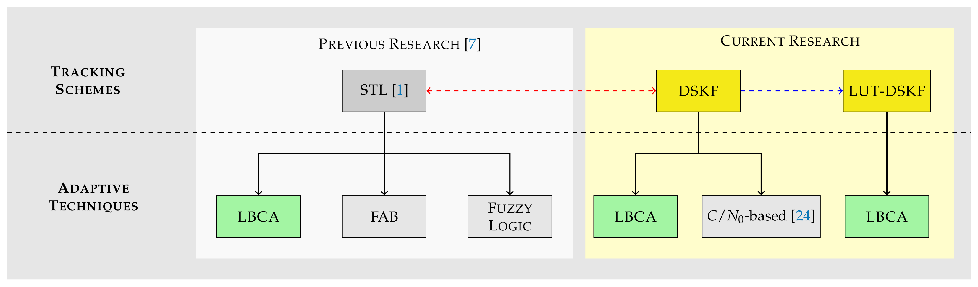
Figure 1 presents a roadmap of the studies. Previous research [7] evaluated three adaptive tracking techniques in the standard STL: the loop-bandwidth control algorithm (LBCA), the fast adaptive bandwidth (FAB), and the Fuzzy logic. The LBCA was superior to the other techniques regarding tracking performance, system performance, and complexity. This technique adjusts the STL’s loop bandwidth based on the statistics of the discriminator’s output [28]. The current research extends the LBCA by implementing it in the DSKF. The relationship between the STL and the DSKF, referred to as the dashed red line, facilitates the LBCA’s implementation in the DSKF. The LBCA’s estimated loop bandwidth can be related to and in the steady-state. Suppose one of the covariances is set to a constant value. In that case, the remainder covariance can be updated based on the LBCA’s bandwidth update.
In addition, the DSKF can be simplified considering the convergence of the Kalman gains in the steady-state, referred to as the dashed blue line. This low-complexity tracking scheme is the so-called lookup table (LUT)-DSKF. The LBCA can also be implemented in the LUT-DSKF and directly update the Kalman gains based on the estimated loop bandwidth. This paper evaluates the performance of the LBCA-based DSKF and the LBCA-based LUT-DSKF. These adaptive techniques are compared with the C/N0-based DSKF, a well-known state-of-the-art method that adapts based on the estimated C/N0 [24]. The DSKF, the LUT-DSKF, and the mentioned adaptive techniques are implemented in the carrier phase synchronization tracking stage of the GOOSE© receiver [29]. Each adaptive technique’s tracking performance and system performance are evaluated under simulated scenarios with different dynamics and noise levels. These methods are also compared with the LBCA-based standard STL [7].
This research expands a conference paper [20] by describing in detail the relationship between STL and the DSKF, explaining the DSKF’s steady-state convergence that leads to the LUT-DSKF, adapting the LUT-DSKF using the LBCA, and improving the scope of the results.
The rest of the paper is organized as follows: Section 2 compares the standard STL with the DSKF, analyzes the steady-state convergence and derives the tracking scheme of the LUT-DSKF. Section 3 shows the architecture of the adaptive techniques used in the DSKF and the LUT-DSKF. The experimental setup and implementation in an open software interface GNSS hardware receiver are described in Section 4. Section 5 presents the adaptive tracking techniques’ complexity, tracking performance, and system performance results. These results are discussed in Section 6. Finally, Section 7 concludes and indicates future work.
2. Tracking Scheme of Direct-State Kalman Filter
The DSKF considers the standard STL as part of the KF [15]. This section describes the relation between standard STL and DSKF and analyzes the DSKF’s convergence in the steady-state. First, an overview of the STL’s open-loop state space model (SSM) and transfer function will facilitate the comparison of STL with the DSKF. Second, the DSKF is explained, and the equivalence to a standard STL is proven. Third, the process noise covariance matrix and measurement noise covariance matrix are described. Fourth, the Kalman filter’s discrete algebraic Riccati equation (DARE) solution leads to the relation between the bandwidth B, the Kalman gains , , and . Finally, from the DARE’s solution, the LUT-DSKF is presented.
2.1. Standard Scalar Tracking Loop
The STL’s tracking scheme must be revisited to understand the relationship between the standard STL and the DSKF. Figure 2 shows the block diagram of the STL’s linear model. The comparator is a linearized discriminator that performs the difference between the input signal’s synchronization parameter and the estimated smoothed error :
where n is the sample index, and is the un-smoothed error that outputs the comparator. The loop filter smooths and drives the smoothed error rate to the NCO. Finally, the NCO closes the loop, sending to the comparator. Depending on the type of discriminator, represents the carrier offset (PLL), the frequency Doppler (FLL), or the code phase offset (DLL).
Considering that the backward Euler transform (BET) is used to discretize the STL [30], the open-loop digital SSM representation of a -order STL is expressed as follows:
where is the state vector, is the state transition matrix, is the filter coefficients vector, and is the observation matrix.
To calculate the STL’s open-loop transfer function , the z-transform of Equations (2) and (3) must be performed first:
Finally, the open-loop transfer function is expressed as:
where and indicate the loop filter’s and NCO’s transfer function.
The closed-loop transfer function is related to considering the z-transform of Equation (1):
Figure 3 presents a particular case of the STL with .
Suppose the third-order STL is used for carrier phase synchronization. In that case, , , and represent the carrier phase, carrier Doppler, and carrier Doppler rate.
Moreover, based on Equation (10), the open-loop transfer function of the third-order STL is expressed as:
Consequently, the closed-loop transfer function is calculated based on Equation (11):
2.2. Direct-State Kalman Filter
The DSKF, as in the KF [10,11,12], is divided into two stages: prediction and update. The prediction step estimates the predicted state and predicted error covariance . and are calculated based on the previously updated state , the previously updated error covariance , and the process noise covariance matrix :
where the superscript is the transpose.
The update stage calculates the updated state based on , the measurement residual , and the Kalman gains . comes from the difference between the observations and the estimated measurement based on . The Kalman gains indicate how accurate the measurements are. depends on the predicted error covariance and the measurement noise covariance .
where is the innovation covariance matrix, and is the identity matrix. The order p and the number of measurements m determine the dimension of the presented variables. This paper assumes only one measurement (i.e., ) to compare the DSKF with the STL. In that case, Equation (1) is the same as Equation (19).
Figure 4 shows the linear model of the DSKF considering only one measurement. The innovation block of the DSKF is equivalent to the STL’s comparator of Figure 2. The state prediction and update block marked in green correspond to the STL’s loop filter and NCO. The main difference between the standard STL and the DSKF is the addition of the Kalman gains’ calculation depicted in the dashed yellow block of Figure 4.
2.3. Process and Measurement Noise Covariance Matrix
The Kalman gains are calculated for each loop iteration based on Equations (17), (20), (21) and (23). depends on the process noise covariance and measurement noise covariance . This paper calculates these matrices considering a third-order DSKF for carrier phase tracking. In addition, a constant-acceleration model is assumed [31,32] for the calculation. The BET is used to discretize the noise that is added in the acceleration state:
where is the continuous noise vector, is the discretized noise vector, and is the zero-mean Gaussian distributed perturbation that suffers the acceleration in .
is obtained performing the variance of the discretized noise:
where q is the variance of in and determines the uncertainty of the states. A higher q implies higher state uncertainty, leading to higher confidence in the incoming measurements. On the contrary, a lower the q leads to higher confidence of the states and less dependence on the measurement.
The measurement noise covariance determines the validity of the incoming measurements. A high value indicates an increased uncertainty, whereas a low value defines high confidence. An adequate model for is the Cramér-Rao bound (CRB) of the STL since it represents the minimum error variance of a time of arrival (ToA) unbiased estimator [33,34]. In this case, the measurement residual of the DSKF is the discriminator’s output of an STL. The CRB of is achieved when the error estimation does not feedback on additional noise. Only the thermal noise of the incoming error parameter is present. If the carrier phase offset parameter () is taken as a measurement, and under the assumption of a two-quadrant discriminator, R in is represented as [28,34,35]:
where is the linear C/N0 in Hertz. This relation is commonly used in C/N0-based DSKF [24,25].
2.4. Steady-State Analysis
In the steady-state region, the Kalman gains converge to a steady-state value given a constant q and R. The solution of the DARE presents the relation between , q and R. The expression of the DARE is [36,37]:
where is the steady-state convergence of the error covariance matrix . The following is assumed to facilitate DARE’s solution [19]:
The resulting for a third-order DSKF is symmetric and defined as:
2.5. Equivalent Noise Bandwidth
Assuming that the integration time tends to zero, the digital loop bandwidth is equivalent to the analog loop bandwidth B [38,39,40]. The relation between B and the coefficients of a third-order STL is expressed as:
Substituting Equations (27) and (34) in Equation (36), the relation between the steady-state equivalent noise bandwidth of a third-order DSKF, q, and R is [5]:
2.6. LUT-DSKF
3. Adaptive Techniques in DSKF
This section describes the three adaptive tracking techniques under evaluation: the C/N0-based DSKF, the LBCA-based DSKF, and the LBCA-based LUT-DSKF.
3.1. -Based DSKF
Figure 8 shows the non-linear model diagram of the C/N0-based DSKF. This technique adapts the measurement noise covariance matrix while fixing the process covariance matrix . In the case of a Costas PLL, the measurement noise covariance R depends on the C/N0 and the integration time (see Equation (30)).
There are several methods to calculate the C/N0. The Beaulieu’s method is used due to its estimation accuracy and simplicity to estimate the C/N0 [41,42]. This method is sub-optimal if the carrier phase lock is not achieved. However, it is assumed that the carrier phase is in lock.
where N is the number of observed correlation samples, is the estimated noise power in the correlation, and is the signal-plus-noise power. is represented as:
is the prompt correlation value of the in-phase component. is defined as:
If the noise contribution is small, the instantaneous signal-plus-noise power approximates to the signal’s power.
3.2. LBCA-Based DSKF
Figure 9 shows the architecture of the adaptive DSKF using the LBCA. This technique adapts the loop bandwidth B of the DSKF and, in turn, adapts q while setting R to a constant value based on Equation (37).
In previous studies, the LBCA has been implemented in the standard STL [28]. The LBCA-based STL presented superior tracking and system performance compared to other state-of-the-art techniques while achieving the lowest complexity [7]. This technique adapts the loop bandwidth based on a normalized bandwidth-dependent weighted difference between estimated noise and estimated signal dynamics. The normalized bandwidth is the product between the integration time and the loop bandwidth B:
First, the absolute mean and the standard deviation of the discriminator’s output are estimated. Second, the normalized dynamics are calculated:
Third, the difference between the normalized dynamics and a normalized-bandwidth-dependent weighting function is performed:
where c is the control value and indicates the maximum value of . Finally, the control value updates the current normalized bandwidth :
where is the updated loop bandwidth. The noisy mean and standard deviation estimates can induce some noise instabilities into the updated loop bandwidth. Therefore, a Schmitt trigger is included to reduce these noise instabilities. The Schmitt trigger changes the next loop bandwidth by if the absolute difference between the updated loop bandwidth and the actual exceed :
Based on the relationship between R, q, and the steady-state loop bandwidth from Equation (37), the updated q can be calculated:
3.3. LBCA-Based LUT-DSKF
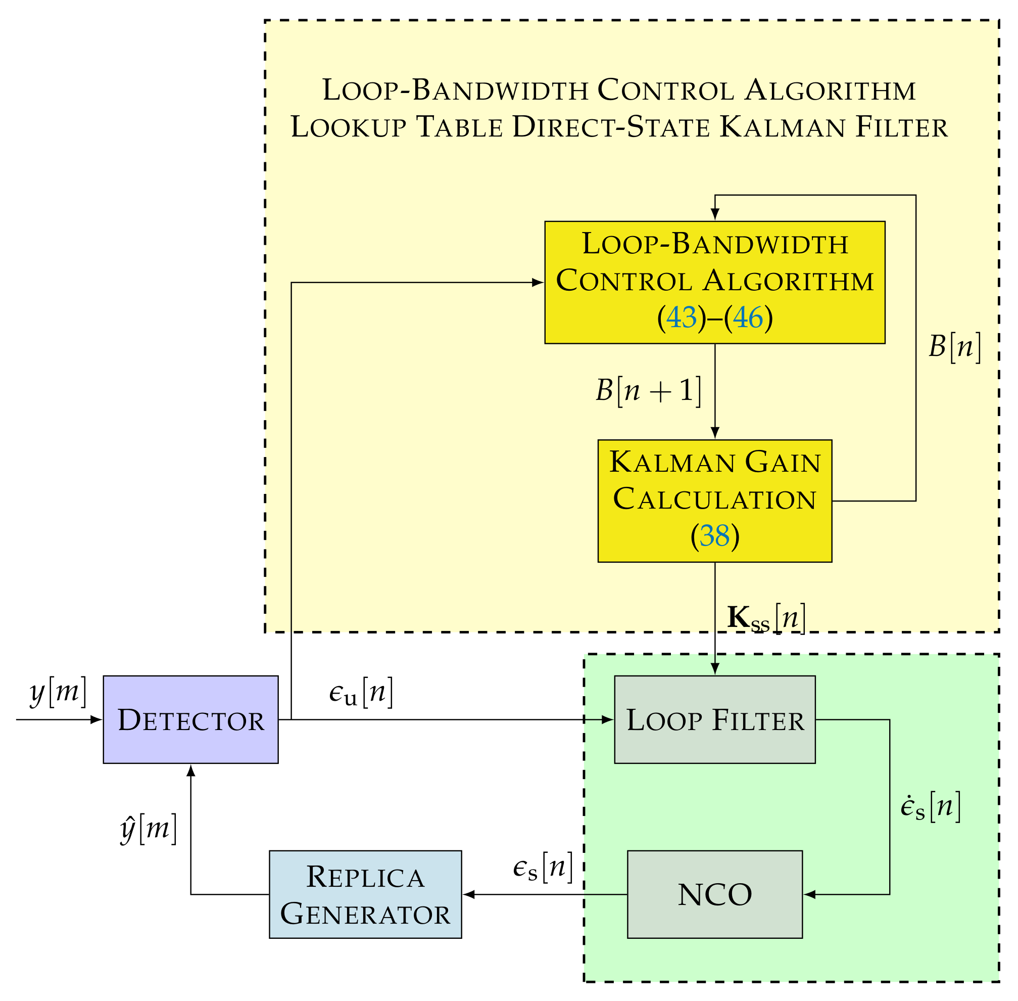
The convergence of the DSKF’s Kalman gains at the steady-state region can reduce the complexity of the algorithm. From the DARE equation (see Equation (31)), the relation between the steady-state Kalman gains , q, and R can be derived (see Equation (34)). This relation simplifies the algorithm as shown in Figure 7. Figure 10 presents the LBCA-based LUT-DSKF. The same steps as in the LBCA-based DSKF to calculate the updated loop bandwidth are followed (see Equations (43)–(46)). In contrast to the LBCA-based DSKF, the mapping between Kalman gains and loop bandwidth is directly done using Equation (38).
4. Experimental Setup
This section describes the GNSS receiver under test, the configuration of each presented adaptive algorithm, the metric used to determine the tracking and system performance, and the simulated scenarios.
4.1. Receiver and Algorithm Implementation
The GOOSE© platform, developed by Fraunhofer IIS and marketed through TeleOrbit GmbH, is a GNSS receiver with an open software interface [29,43]. A picture of the receiver is shown in Figure 11. The receiver contains a customized tri-band radio-frequency front-end (RFFE), a Xilinx Kintex7 field-programmable gate array (FPGA), and a dualcore ARM processor. The RFFE amplifies, filters, downconverts, discretizes the GNSS signals, and sends the digital samples to the FPGA. The analog-to-digital converter (ADC) discretizes each frequency band at a sample rate of 81 MHz and a resolution of 8 bits. The FPGA includes one acquisition module and sixty tracking channels, which the processor can control. The processor performs the acquisition of the incoming digital samples using the acquisition module of the FPGA. The tracking starts once the acquisition achieves a rough estimate of the frequency Doppler and code phase . The tracking stage of this GNSS receiver is partially implemented in the FPGA (e.g., correlators and NCO) and software (e.g., discriminators and loop filters). This stage consists of three steps. First, the FLL and the DLL refine the acquired and estimates. Second, the PLL starts and synchronizes with the carrier phase. Finally, the FLL stops and the PLL works unaided when the latter successfully achieves a good lock with the carrier phase. The receiver synchronizes with the navigation data at this stage, and the integration time increases to the symbol period. In the case of Global Positioning System (GPS) L1 C/A, the integration time is increased to 20 ms.
The C/N0-based DSKF, the LBCA-based DSKF, and the LBCA-based LUT-DSKF are implemented in the third-order Costas PLL of the GOOSE receiver in software.
4.1.1. -Based DSKF Configuration
The time of response of the C/N0 estimation determines the agility of the measurement’s covariance update. This parameter changes according to the accumulated correlation samples N (see Equation (39)). This study evaluates this method’s tracking and system performance with samples and samples. Using an integration time of 20 ms, the response time of the C/N0’s estimate is 2 s and 10 s, respectively. The steady-state process variance q is set to a constant value. Different values of q are evaluated since this parameter directly impacts on the robustness to signal dynamics.
4.1.2. LBCA-Based DSKF and LUT-DSKF Configuration
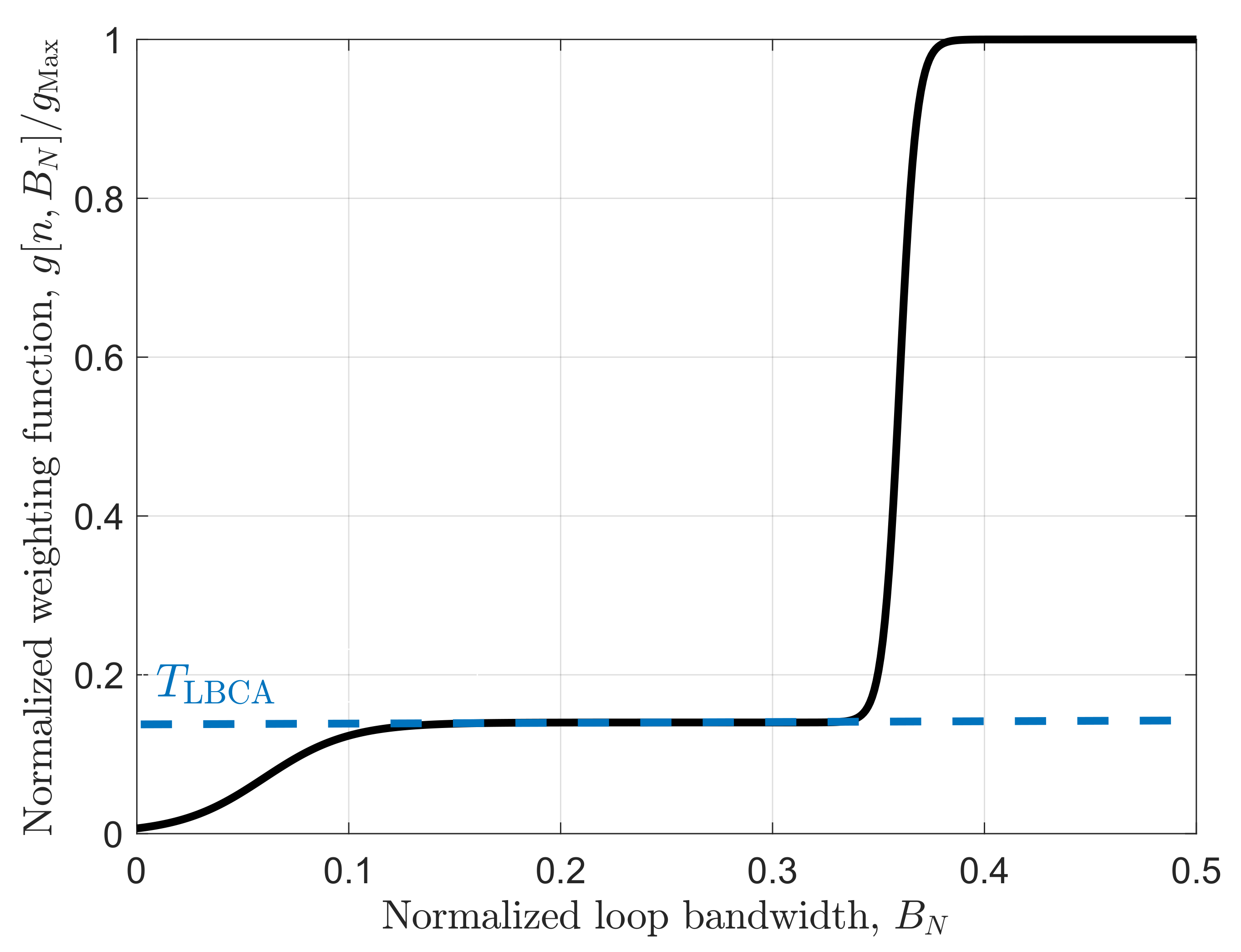
The selected weighting function is a linear combination of two Sigmoid functions and has the following expression:
where is the Sigmoid function [44]. Figure 12 shows the graphical representation of Equation (48). is the normalized dynamic threshold and indicates the sensitivity of the algorithm to signal dynamics. In this case, is set to 0.1 and to 0.14. This weighting function presented the best results in the LBCA-based PLL [7].
4.2. Performance Metric
The metric to evaluate the PLL tracking and system performance is the same as in previous studies [7]. The tracking performance evaluates the tracking of a single satellite vehicle ( SV), whereas the system performance considers all the visible SV. in meters is characterized as:
where is the wavelength of the GPS L1 C/A signal, is the average of the last ten minutes un-smoothed carrier phase error’s standard deviation, and is the square root of the CRB [7]. in cycles is defined as:
where is the number of evaluation epochs in samples. The total evaluation time in seconds is:
where is the data-logging rate in Hertz.
in cycles is represented as:
where the term is the squaring loss [1].
The three-sigma rule-of-thumb conservative upper threshold is considered in the tracking performance evaluation. For a two-quadrant phase discriminator, in cycles is expressed as:
A low value of denotes good tracking performance. If the measured from is less than considering , one can ensure stable tracking and no cycle slips [1]. On the contrary, if the measured is bigger than the conservative threshold, the probability of losing the lock increases.
The metric used for the system performance is expressed as:
where is the average of the phase-lock indicator (PLI) with respect and the accumulated number of tracked SV , and is the normalized average number of visible satellites being tracked.
The expression of is:
and is calculated based on the prompt in-phase and prompt quadrature correlation samples of the corresponding SV:
The second term of Equation (54), , is defined as:
where is the total number of SV during the simulation.
and are normalized. Consequently, is also normalized. A value near to one of refers to good system performance, whereas a value near zero indicates poor system performance and the possibility of not achieving a PVT solution. The average of with respect to the C/N0 levels leads to a comprised metric that evaluates the overall system performance of an adaptive tracking technique:
where is the number of C/N0 levels.
4.3. Evaluation Setup
The evaluation setup is the same as in previous studies [7,20,28]. The Spirent GSS9000 radio-frequency constellation simulator (RFCS) generates controlled scenarios at different C/N0 and signal dynamics levels. The simulator is configured to perform 20 min simulations of a specific scenario at eight different C/N0 levels (). In contrast to previous studies, the selected C/N0 levels are {25, 29, 33, 37, 41, 45, 48, 52} dBHz. The simulation always starts at the highest C/N0 level of 52 dBHz to ensure successful signal acquisition. Next, the C/N0 level is reduced in 30 second intervals until reaching the desired C/N0 level. The tracking and system performance are measured considering the last ten minutes of the simulation, 600 s, in which the correct C/N0 level is assured.
A static scenario and a dynamic scenario are selected to evaluate the adaptive tracking techniques. The static scenario represents stationary use-cases such as GNSS reference stations, and the dynamic scenario presents harsh vehicular conditions. Figure 13 shows the sky-plots of both scenarios. In the static scenario there are nine SVs during the entire simulation (see Figure 13a). However, SV G1 disappears behind the horizon after two minutes of the simulation. The dynamic scenario shows ten visible SVs (see Figure 13b). As in the static scenario, SV G1 disappears after two minutes of the simulation. Moreover, SV G30 rises above the horizon near the end of the simulation. Therefore, to avoid these transient SVs, SV G1 and SV G30 are not considered, and is set to eight for both scenarios.
The same SV as previous research are selected to evaluate the tracking performance [7]. The GPS L1 C/A signal of SV G4 is selected to evaluate the static tracking performance, and the GPS L1 C/A signal of SV G17 is assigned for the dynamic tracking performance. The maximum line-of-sight (LOS) signal dynamics for the dynamic simulated scenario is 8.7 g/s [7].
5. Results
This section evaluates the tracking performance, system performance, number of operations, and time complexity of the adaptive tracking techniques in the DSKF. The dataset used to plot the presented results are available on the cloud [45].
5.1. Static Scenario
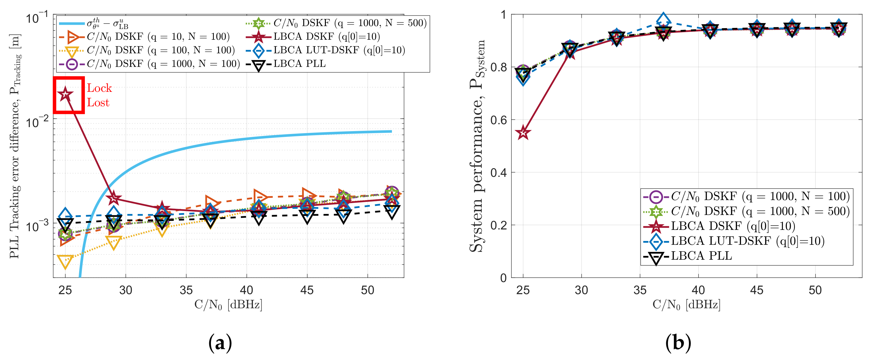
Figure 14 presents the tracking performance and system performance of the implemented adaptive techniques in a stationary scenario. Four configurations of the C/N0-based DSKF using different steady-state process noise variances () and different correlation samples () are evaluated. Moreover, the LBCA-based DSKF, and the LBCA-based LUT-DSKF are analyzed using the weighting function defined in Equation (48). These adaptive tracking techniques are compared with the LBCA-based STL using the same weighting function.
Figure 14a shows that all the presented configurations of the C/N0-based DSKF do not lose the lock at any C/N0 level. The number of correlation samples N does not impact the static tracking performance. In contrast, q has an effect at low C/N0 levels. An intermediate value of achieves the lowest results, meaning the best tracking performance. In the LBCA-based DSKF, q starts with an initial value of 10 and is adapted based on the LBCA’s loop bandwidth update, while R is fixed to . At high C/N0 levels, this method presents the same tracking performance as the other techniques. However, at low C/N0 levels, increases significantly, until finally losing the lock at 25 dBHz. The LBCA-based LUT-DSKF does not lose the lock at low C/N0 levels, but it does not perform better than the C/N0-based DSKF. The LBCA-based STL performs best at high C/N0 levels, but the performance deteriorates at low C/N0 levels. The weighting function of the LBCA is configured to be robust to signal dynamics, with the cost of a worse performance at low C/N0 levels.
Figure 14b discloses each adaptive tracking technique’s system performance (see Equation (54)). All the configurations show a good system performance above 0.8, except for the LBCA-based DSKF at 25 dBHz. While the system performance of this technique at 25 dBHz is lower than 0.6, the PVT has not been lost.
5.2. Dynamic Scenario
Figure 15 displays the tracking and system performance of the adaptive techniques in a dynamic scenario. SV G17 is challenging to track due to the high LOS jerk dynamics. From Figure 15a, it is observed that a high q and N are required in the C/N0-based DSKF to maintain the carrier phase synchronization lock. The C/N0-based DSKF achieves best tracking performance with and a 500 samples, maintaining the lock until 45 dBHz. The LBCA-based DSKF keeps the lock until 38 dBHz. However, this technique presents an error bias compared to the other techniques. This bias exists due to the transitions between the update of q and the Kalman gains’ convergence. In contrast to the latter technique, the LBCA-based LUT-DSKF does not contain any error bias, and it performs almost as well as the LBCA-based PLL, keeping the lock until 33 dBHz. The LBCA-based PLL has a superior dynamic tracking performance than the other techniques due to the direct relation between loop bandwidth and filter coefficients. This direct relationship leads to a faster reaction of high signal dynamics.
The results of the dynamic system performance (see Figure 15b) are consonant with the dynamic tracking performance. All the adaptive tracking techniques can achieve a PVT solution at high C/N0 levels (38–52 dBHz). The LBCA-based LUT-DSKF and the LBCA-based PLL have the best system performance results, whereas the C/N0-based DSKF technique shows poor performance. At low C/N0 levels, the LBCA-based techniques almost achieve a continuous PVT at 33 dBHz. In contrast to the LBCA-based methods, the C/N0-based DSKF only achieves a continuous tracking of one SV.
5.3. Total System Performance
5.4. Complexity
Table 2 shows the added number of additions, multiplications, and divisions required for each adaptive technique in the DSKF compared to the standard STL. The total number of operations is marked as red, orange, and green, depending on the level of complexity. The colors vary from the most complex one, marked in red, to the simplest one, marked in green.
The presented equivalence between the DSKF and the standard STL (see Figure 4 and Figure 5) shows that only the Kalman gain calculation (i.e., yellow block of Figure 4) must be included. The C/N0-based DSKF adapts R based on Equation (30), being q a constant value. In contrast, the LBCA-based DSKF set R to a constant value, while adapting q using the LBCA. This technique needs additional complexity to map the loop bandwidth with the steady-state process variance q (see Equation (47)).
The LUT-DSKF significantly reduces the complexity by calculating the convergence of the Kalman gains in the steady-state. In the LBCA-based LUT-DSKF, the relation between the B and is used (see Equation (38)) to update the filter coefficients.
In all the LBCA-based techniques, the weighting function of the LBCA technique is approximated using the piecewise linear approximation of nonlinearities (PLAN) technique [7].
Table 3 shows the time complexity of the standard PLL and each adaptive tracking technique. The time complexity measures the algorithm’s processing time in software on the processing platform. The same procedure as in previous research is carried out [7]. An Intel Skylake micro-architecture with a clock speed of 3700 MHz is used to evaluate the time complexity of each technique. The code is implemented in C++, and a for-loop is used to iterate the operation of a loop filter times. The processing time of each method is measured using the chrono library [46], and the operf Linux profiler tool is used to analyze the utilization of the used libraries during the algorithm’s execution [47]. In addition, the taskset command is used to bind the application process to one single core [48].
Three parameters are shown in Table 3. First, the total time complexity in seconds. Second, the average time complexity at each iteration in nanoseconds:
Finally, the added time complexity compared to the standard loop filter :
While this approach depends on how exemplary the algorithm’s software implementation is, the results show a correlation between the number of operations and the time complexity.
6. Discussion
Figure 16 compares the average system performance and the added time complexity of the presented adaptive tracking techniques implemented in a third-order DSKF for carrier phase tracking. These graphs summarize the collected results combining Table 1 and Table 3.
Figure 16a shows that the LBCA-based DSKF have the worst and the highest . In contrast, the LBCA-based LUT-DSKF achieves the best static , although its complexity is higher than the LBCA-based standard PLL . The state-of-the-art C/N0-based DSKF have similar , and is between and . presents the lowest with a slightly worse than .
In the dynamic scenario, the superior performance of the LBCA-based techniques is clearly observed in Figure 16b. In this case, and present the worst . In a highly dynamic event, the carrier tracking loop cannot follow the phase dynamics, leading to a fast shift from in-phase to quadrature component. In such a moment, the C/N0 estimate of Beaulieu’s method drops. Consequently, R increases, and the DSKF wrongly stops trusting the incoming carrier phase measurement. This leads to a loss of the carrier lock. In Figure 15a, a greater number of the accumulated correlation samples N and q improves the robustness to dynamics. Then, a further evaluation with higher q and N should improve in the dynamic scenario. Among the LBCA-based techniques, performs the worst. Once adapts q, time is needed to adjust the Kalman gains to the steady-state values. Due to this latency, is not fast enough to adapt its coefficients in time, leading to a higher risk of losing the lock at high dynamic scenarios. experiences no latencies since the steady-state Kalman gains are directly set based on the loop bandwidth update. This method achieves the best , followed by .
The scope of this research is to show the extension of the LBCA by applying it to the DSKF. While this has been shown, adding the LBCA into the DSKF to adapt q while fixing R does not present remarkable results, and the complexity increases significantly. Therefore, other methods have been considered to improve the performance and reduce the complexity. The LBCA-based LUT-DSKF presents superior static and dynamic among the rest of the adaptive tracking techniques. However, the LBCA-based PLL is less complex than the LBCA-based LUT DSKF, with a slight reduction of the total system performance in both static and dynamic scenarios.
7. Conclusions
This study presents the first proof of the LBCA’s general applicability to any control system by implementing it in the DSKF. First, the relation between the standard STL and the DSKF is presented. Second, DARE’s solution relates the DSKF’s loop bandwidth, the noise covariances, and the Kalman gains in the steady-state. This relationship eases the implementation of the LBCA into the DSKF, and two approaches are presented: The LBCA-based DSKF and the LBCA-based LUT-DSKF. The LBCA-based DSKF uses the LBCA to adapt q for each loop iteration while setting R to a constant value. In contrast, the LBCA-based LUT-DSKF directly relates the LBCA’s loop bandwidth update and the Kalman gains. These adaptive tracking techniques have been evaluated in a third-order Costas PLL. These techniques’ complexity and static and dynamic system performance are compared with the state-of-the-art C/N0-based DSKF and the LBCA-based standard STL [7]. Results show the superior performance of the LBCA-based LUT-DSKF compared to the other techniques. In terms of complexity, the LBCA-based LUT-DSKF presents less complexity compared to the other adaptive DSKFs. However, this method has greater added time complexity than the LBCA-based standard PLL. In further research, Equation (38) will be merged into the STL to achieve similar time complexity.
An extension of the presented tracking schemes is the implementation of a LUT-DSKF that encloses the DLL, FLL, and PLL of a tracking channel. The use of the LBCA in this tracking architecture can improve the tracking performance in scenarios with different noise and signal dynamics. To cope with scenarios with multipath effects (e.g., in urban scenarios), a multi-frequency LUT-DSKF will be proposed, and the addition of the LBCA will be evaluated. Furthermore, an evaluation in real scenarios of all the LBCA-based techniques will lead to the final verification of the LBCA.
This paper opens the door to a range of applications of the LBCA where the KF is involved. The LBCA can be implemented in the tracking stage, the interference mitigation stage (e.g., adaptive notch filtering), and the post-processing stage (e.g., adaptive loose and tightly coupling solutions) of a GNSS receiver.
Author Contributions
Conceptualization, I.C.; methodology, I.C. and J.R.v.d.M.; software, I.C.; validation, I.C.; formal analysis, I.C.; investigation, I.C. and J.R.v.d.M.; resources, I.C.; data curation, I.C.; writing–original draft preparation, I.C.; writing–review and editing, I.C., J.R.v.d.M., E.S.L.; visualization, I.C.; supervision, J.N., E.S.L.; project administration, W.F.; funding acquisition, W.F. All authors have read and agreed to the published version of the manuscript.
Funding
This research received no external funding.
Institutional Review Board Statement
Not applicable.
Informed Consent Statement
Not applicable.
Data Availability Statement
Publicly available datasets were analyzed in this study. This data can be found here: https://owncloud.fraunhofer.de/index.php/s/LGoWPVtV5xbQ9mB (accessed on 14 December 2020).
Conflicts of Interest
The authors declare no conflict of interest.
Abbreviations
The following abbreviations are used in this manuscript:
| ADC | analog-to-digital converter |
| BET | backward Euler transform |
| carrier-to-noise density ratio | |
| CRB | Cramér-Rao bound |
| DARE | discrete algebraic Riccati equation |
| DLL | delay locked loop |
| DSKF | direct-state Kalman filter |
| ESKF | error-state Kalman-filter |
| FAB | fast adaptive bandwidth |
| FLL | frequency locked loop |
| FPGA | field-programmable gate array |
| GNSS | global navigation satellite system |
| GPS | Global Positioning System |
| IIR | infinite impulse response |
| KF | Kalman filter |
| LBCA | loop-bandwidth control algorithm |
| LOS | line-of-sight |
| LUT | lookup table |
| MMSE | minimum mean square error |
| NCO | numerically controlled oscillator |
| PLAN | piecewise linear approximation of nonlinearities |
| PLI | phase-lock indicator |
| PLL | phase locked loop |
| PVT | position, velocity, and time |
| RFCS | radio-frequency constellation simulator |
| RFFE | radio-frequency front-end |
| SSM | state space model |
| STL | scalar tracking loop |
| SV | satellite vehicle |
References
- Kaplan, E.D.; Hegarty, C.J. Understanding GPS: Principles and Applications, 2nd ed.; Artech House Mobile Communications Series; Artech House: Norwood, MA, USA, 2006. [Google Scholar]
- Van Dierendonck, A.J. GPS Receivers. In Global Positioning System: Theory and Applications; American Institute of Aeronautics and Astronautics, AJ Systems: Los Altos, CA, USA, 1996; Volume 1. [Google Scholar] [CrossRef]
- Won, J.; Pany, T. Signal Processing. In Springer Handbook of Global Navigation Satellite Systems; Springer International Publishing: Cham, Switzerland, 2017; pp. 401–442. [Google Scholar] [CrossRef]
- Jade Morton, Y.T.; Yang, R.; Breitsch, B. GNSS Receiver Signal Tracking. In Position, Navigation, and Timing Technologies in the 21st Century: Integrated Satellite Navigation, Sensor Systems, and Civil Applications; Wiley-IEEE Press, University of Colorado Boulder: Hoboken, NJ, USA, 2021; Volume 1. [Google Scholar]
- Jwo, D.J. Optimisation and sensitivity analysis of GPS receiver tracking loops in dynamic environments. IEE Proc. Radar Sonar Navig. 2001, 148, 241–250. [Google Scholar] [CrossRef] [Green Version]
- Gardner, F.M. Phaselock Techniques, 3rd ed.; Wiley: New York, NY, USA, 2005. [Google Scholar]
- Cortés, I.; van der Merwe, J.R.; Nurmi, J.; Rügamer, A.; Felber, W. Evaluation of adaptive loop-bandwidth tracking techniques in GNSS receivers. Sensors 2021, 21, 502. [Google Scholar] [CrossRef]
- López-Salcedo, J.A.; Peral-Rosado, J.A.D.; Seco-Granados, G. Survey on robust carrier tracking techniques. IEEE Commun. Surv. Tutor. 2014, 12, 670–688. [Google Scholar] [CrossRef]
- Vilà-Valls, J.; Linty, N.; Closas, P.; Dovis, F.; Curran, J.T. Survey on signal processing for GNSS under ionospheric scintillation: Detection, monitoring, and mitigation. Navigation 2020, 67, 511–536. [Google Scholar] [CrossRef]
- Driessen, P.F. DPLL bit synchronizer with rapid acquisition using adaptive Kalman filtering techniques. IEEE Trans. Commun. 1994, 42, 2673–2675. [Google Scholar] [CrossRef]
- Gelb, A. The Analytic Sciences Corporation. In Applied Optimal Estimation; The MIT Press: Cambridge, MA, USA, 1974. [Google Scholar]
- Thacker, N.A.; Lacey, A.J. Tutorial: The Likelihood Interpretation of the Kalman Filter; Tina Memo; University of Manchester: Manchester, UK, 2006. [Google Scholar]
- Vilà-Valls, J.; Closas, P.; Navarro, M.; Fenández-Prades, C. Are PLLs dead? A tutorial on Kalman filter-based techniques for digital carrier synchronization. IEEE Aerosp. Electron. Syst. 2017, 32, 28–45. [Google Scholar] [CrossRef]
- Won, J.H.; Dötterböck, D.; Eissfeller, B. Performance comparison of different forms of Kalman filter approaches for a vector-based GNSS signal tracking loop. Navigation 2010, 57, 185–199. [Google Scholar] [CrossRef]
- Won, J.-H.; Pany, T.; Eissfeller, B. Characteristics of Kalman filters for GNSS signal tracking loop. IEEE Aerosp. Electron. Syst. 2012, 48, 3671–3681. [Google Scholar] [CrossRef]
- O’Driscoll, C.; Lachapelle, G. Comparison of traditional and Kalman filter based tracking architectures. In Proceedings of the 2009 European Navigation Conference (ENC), Warsaw, Poland, 3–6 May 2009. [Google Scholar]
- O’Driscoll, C.; Petovello, M.; Lachapelle, G. Choosing the coherent integration time for Kalman filter based carrier phase tracking of GNSS signals. GPS Solut. 2011, 15, 345–356. [Google Scholar] [CrossRef]
- Tang, X.; Falco, G.; Falletti, E.; Lo Presti, L. Theoretical analysis and tuning criteria of the Kalman filter-based tracking loop. GPS Solut. 2014, 19, 489–503. [Google Scholar] [CrossRef]
- Tang, X.; Falco, G.; Falletti, E.; Lo Presti, L. Complexity reduction of the Kalman filter-based tracking loops in GNSS receivers. GPS Solut. 2017, 21, 685–699. [Google Scholar] [CrossRef]
- Cortés, I.; Marín, P.; van der Merwe, J.R.; Lohan, E.S.; Nurmi, J.; Felber, W. Adaptive techniques in scalar tracking loops with direct-state Kalman-filter. In Proceedings of the 2021 International Conference on Localization and GNSS (ICL-GNSS), Tampere, Finland, 1–3 June 2021; pp. 1–7. [Google Scholar] [CrossRef]
- Vilà-Valls, J.; Closas, P.; Fenández-Prades, C. On the identifiability of noise statistics and adaptive KF design for robust GNSS carrier tracking. In Proceedings of the 2015 IEEE Aerospace Conference, Big Sky, MT, USA, 7–14 March 2015; pp. 1–10. [Google Scholar] [CrossRef]
- Duník, J.; Straka, O.; Kost, O.; Havlík, J. Noise covariance matrices in state-space models: A survey and comparison of estimation methods—Part I. Int. J. Adapt. Con. Sig. Proc. 2017, 31, 1505–1543. [Google Scholar] [CrossRef]
- Bolla, P. Advanced Tracking Loop Architectures for Multi-Frequency GNSS Receiver. Ph.D. Thesis, Tampere University of Technology, Tampere, Finland, 2018. [Google Scholar]
- Won, J.W.; Eissfiller, B. A tuning method based on signal-to-noise power ratio for adaptive PLL and its relationship with equivalent noise bandwidth. IEEE Commun. Lett. 2013, 17, 393–396. [Google Scholar] [CrossRef]
- Won, J.H. A novel adaptive digital phase-lock-loop for modern digital GNSS receivers. IEEE Commun. Lett. 2014, 18, 46–49. [Google Scholar] [CrossRef]
- Susi, M.; Borio, D. Kalman filtering with noncoherent integrations for Galileo E6-B tracking. Navigation 2020, 67, 601–618. [Google Scholar] [CrossRef]
- Song, Q.; Liu, R. Weighted adaptive filtering algorithm for carrier tracking of deep space signal. Chin. J. Aerosp. 2015, 28, 1236–1244. [Google Scholar] [CrossRef] [Green Version]
- Cortes, I.; Van der Merwe, J.R.; Rügamer, A.; Felber, W. Adaptive loop-bandwidth control algorithm for scalar tracking loops. In Proceedings of the 2020 IEEE/ION Position, Location and Navigation Symposium (PLANS), Portland, OR, USA, 20–23 April 2020; pp. 1178–1188. [Google Scholar] [CrossRef]
- Overbeck, M.; Garzia, F.; Popugaev, A.; Kurz, O.; Forster, F.; Felber, W.; Ayaz, A.S.; Ko, S.; Eissfeller, B. GOOSE-GNSS Receiver with an open software interface. In Proceedings of the 28th International Technical Meeting of the Satellite Division of The Institute of Navigation (ION GNSS+ 2015), Tampa, FL, USA, 14–18 September 2015. [Google Scholar]
- Jury, E.I. Theory and Application of the Z-Transform Method; Wiley: New York, NY, USA, 1964. [Google Scholar]
- Gajic, Z. Linear Dynamic Systems and Signals; Prentice Hall: Upper Saddle River, NJ, USA, 2002. [Google Scholar]
- Reid, I.; Term, H. Estimation II. Available online: https://www.robots.ox.ac.uk/~ian/Teaching/Estimation/LectureNotes2.pdf (accessed on 14 December 2020).
- Kay, S.M. Fundamentals of Statistical Signal Processing: Estimation Theory; Prentice-Hall Signal Processing Series; Prentice Hall: Upper Saddle River, NJ, USA, 1993; Volume 1. [Google Scholar]
- Betz, J.W.; Kolodziejski, K.R. Generalized theory of code tracking with an early-late discriminator Part I: Lower bound and coherent processing. IEEE Trans. Aerosp. Electron. Syst. 2009, 45, 1538–1556. [Google Scholar] [CrossRef]
- D’Andrea, A.N.; Mengali, U.; Reggiannini, R. The modified Cramer-Rao bound and its application to synchronization problems. IEEE Trans. Commun. 1994, 42, 1391–1399. [Google Scholar] [CrossRef]
- Einicke, G. Smoothing, Filtering and Prediction: Estimating the Past, Present and Future; InTech: Rijeka, Croatia, 2012. [Google Scholar]
- Brown, R.G.; Hwang, P.Y.C. Introduction to Random Signals and Applied Kalman Filtering: With MATLAB Exercises and Solutions, 3rd ed.; Wiley: New York, NY, USA, 1997. [Google Scholar]
- Gradshteyn, I.S.; Ryzhik, I.M. Table of Integrals, Series, and Products, 8th ed.; Elsevier: Waltham, MA, USA, 2014. [Google Scholar]
- Stephens, S.; Thomas, J. Controlled-root formulation for digital phase-locked loops. IEEE Trans. Aerosp. Electron. Syst. 1995, 31, 78–95. [Google Scholar] [CrossRef]
- Mao, W.L.; Chen, A.B. Mobile GPS carrier phase tracking using a novel intelligent dual-loop receiver. Int. J. Satell. Commun. Netw. 2008, 26, 119–139. [Google Scholar] [CrossRef]
- Beaulieu, N.C.; Toms, A.S.; Pauluzzi, D.R. Comparison of four SNR estimators for QPSK modulations. IEEE Commun. Lett. 2000, 4, 43–45. [Google Scholar] [CrossRef]
- Falletti, E.; Pini, M.; Presti, L.L. Low complexity carrier-to-noise ratio estimators for GNSS digital receivers. IEEE Trans. Aerosp. Electron. Syst. 2011, 47, 420–437. [Google Scholar] [CrossRef]
- Seybold, J. GOOSE: Open GNSS Receiver Platform; Technical Report; TeleOrbit GmbH: Nuremberg, Germany, 2021; Available online: https://teleorbit.eu/en/satnav/ (accessed on 14 December 2020).
- Domingos, P. The Master Algorithm: How the Quest for the Ultimate Learning Machine Will Remake Our World; Basic Books, Inc.: New York, NY, USA, 2018. [Google Scholar]
- Robust Tracking Techniques Dataset Using GOOSE Receiver. Available online: https://owncloud.fraunhofer.de/index.php/s/LGoWPVtV5xbQ9mB (accessed on 14 December 2020).
- Josuttis, N.M. The C++ Standard Library: A Tutorial and Reference, 2nd ed.; Addison-Wesley Professional: Boston, MA, USA, 2012. [Google Scholar]
- OProfile Manual. Available online: https://oprofile.sourceforge.io/doc/index.html (accessed on 14 December 2020).
- Taskset(1)—Linux Manual Page. Available online: https://man7.org/linux/man-pages/man1/taskset.1.html (accessed on 14 December 2020).
Figure 1.
Research roadmap and comparison to other publications.

Figure 2.
Linear model of the scalar tracking loop (STL).

Figure 3.
Linear model of a third-order STL.

Figure 4.
Linear model of the direct-state Kalman filter (DSKF) with . ©IEEE. Adapted, with permission, from [20].
Figure 4.
Linear model of the direct-state Kalman filter (DSKF) with . ©IEEE. Adapted, with permission, from [20].

Figure 5.
Linear model equivalence between a third-order DSKF and a third-order STL. ©IEEE. Adapted, with permission, from [20].
Figure 5.
Linear model equivalence between a third-order DSKF and a third-order STL. ©IEEE. Adapted, with permission, from [20].

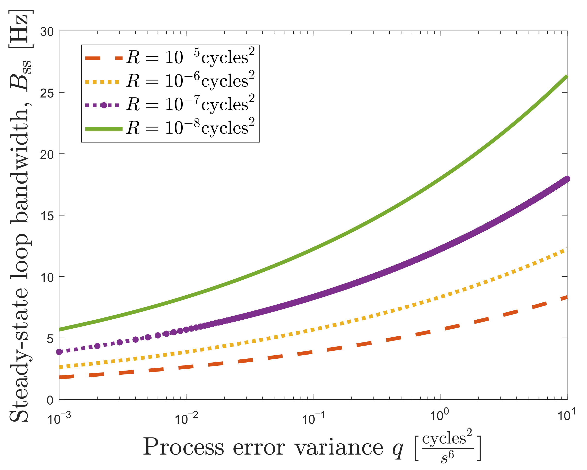
Figure 6.
Relation between steady-state loop bandwidth and process error variance q in a third-order DSKF. ©IEEE. Adapted, with permission, from [20].
Figure 6.
Relation between steady-state loop bandwidth and process error variance q in a third-order DSKF. ©IEEE. Adapted, with permission, from [20].

Figure 7.
Linear model of lookup table (LUT)-DSKF.

Figure 8.
Non-linear model of the carrier-to-noise density ratio ()-based DSKF.

Figure 9.
Non-linear model of loop-bandwidth control algorithm (LBCA)-based DSKF. ©IEEE. Adapted, with permission, from [20].
Figure 9.
Non-linear model of loop-bandwidth control algorithm (LBCA)-based DSKF. ©IEEE. Adapted, with permission, from [20].

Figure 10.
Non-linear model of LBCA-based LUT-DSKF.

Figure 11.
Photo of the GOOSE receiver @Fraunhofer IIS/Paul Pulkert.

Figure 12.
Selected Normalized weighting function in LBCA-based techniques.

Figure 13.
Sky-plot of simulated scenario. (a) Static Scenario. (b) Dynamic Scenario.

Figure 14.
Static performance of adaptive tracking techniques in third-order Costas phase locked loop (PLL) at different C/N0 levels. (a) Tracking performance of satellite vehicle (SV) G4. (b) System performance.
Figure 14.
Static performance of adaptive tracking techniques in third-order Costas phase locked loop (PLL) at different C/N0 levels. (a) Tracking performance of satellite vehicle (SV) G4. (b) System performance.

Figure 15.
Dynamic performance of adaptive tracking techniques in third-order Costas PLL at different C/N0 levels. (a) Tracking performance of SV G17. (b) System performance.
Figure 15.
Dynamic performance of adaptive tracking techniques in third-order Costas PLL at different C/N0 levels. (a) Tracking performance of SV G17. (b) System performance.

Figure 16.
System performance vs. added time complexity comparison. (a) Static scenario. (b) Dynamic scenario.
Figure 16.
System performance vs. added time complexity comparison. (a) Static scenario. (b) Dynamic scenario.


Table 1.
Overall system performance of adaptive tracking techniques.
| Tracking | Configuration | Label | ||
|---|---|---|---|---|
| Technique | Static | Dynamic | ||
| -based DSKF | , | 0.910 | 0.535 | |
| , | 0.909 | 0.538 | ||
| LBCA-based DSKF | , | 0.877 | 0.583 | |
| LBCA-based LUT-DSKF | , | 0.912 | 0.628 | |
| LBCA-based PLL | , | 0.911 | 0.627 |
Table 2.
Complexity of adaptive tracking techniques based on the added number of operations.
| Tracking | Sub- | Added Number of Operations: | ||
|---|---|---|---|---|
| Technique | Module | Additions | Multiplications | Divisions |
| -based DSKF | Error Cov. Prediction (17) | 27 | 18 | - |
| Kalman Gain Calculation (20) and (21) | 1 | 3 | 1 | |
| Error Cov. Update (23) | 9 | 9 | - | |
| Measurement Noise Cov. (30) | 1 | 5 | 2 | |
| Total | 38 | 35 | 3 | |
| LBCA-based DSKF | Error Cov. Prediction (17) | 27 | 18 | - |
| Kalman Gain Calculation (20) and (21) | 1 | 3 | 1 | |
| Error Cov. Update (23) | 9 | 9 | - | |
| LBCA + PLAN [7] | 6 | 7 | 1 | |
| q and B relation (47) | 0 | 6 | 0 | |
| Total | 45 | 37 | 2 | |
| LBCA-based LUT-DSKF | LBCA + PLAN [7] | 6 | 7 | 1 |
| and B relation (38) | 0 | 9 | 0 | |
| Total | 6 | 16 | 1 | |
| LBCA-based PLL | LBCA + PLAN [7] | 6 | 7 | 1 |
| Total | 6 | 7 | 1 | |
Table 3.
Time complexity of adaptive tracking techniques, iterations.
| Tracking | Total Time Complexity | Iteration Time Complexity | Added Time Complexity |
|---|---|---|---|
| Technique | [s] | [ns] | [times] |
| Standard PLL | 6.8 | 22.7 | 1 |
| -based DSKF | 41.5 | 138.3 | 6.1× |
| LBCA-based DSKF | 61.1 | 203.7 | 8.9× |
| LBCA-based LUT-DSKF | 25.8 | 86 | 3.8× |
| LBCA-based PLL [7] | 16.1 | 53.7 | 2.4× |
Publisher’s Note: MDPI stays neutral with regard to jurisdictional claims in published maps and institutional affiliations. |
© 2022 by the authors. Licensee MDPI, Basel, Switzerland. This article is an open access article distributed under the terms and conditions of the Creative Commons Attribution (CC BY) license (https://creativecommons.org/licenses/by/4.0/).
Share and Cite
MDPI and ACS Style
Cortés, I.; van der Merwe, J.R.; Lohan, E.S.; Nurmi, J.; Felber, W. Performance Evaluation of Adaptive Tracking Techniques with Direct-State Kalman Filter. Sensors 2022, 22, 420. https://0-doi-org.brum.beds.ac.uk/10.3390/s22020420
AMA Style
Cortés I, van der Merwe JR, Lohan ES, Nurmi J, Felber W. Performance Evaluation of Adaptive Tracking Techniques with Direct-State Kalman Filter. Sensors. 2022; 22(2):420. https://0-doi-org.brum.beds.ac.uk/10.3390/s22020420
Chicago/Turabian StyleCortés, Iñigo, Johannes Rossouw van der Merwe, Elena Simona Lohan, Jari Nurmi, and Wolfgang Felber. 2022. "Performance Evaluation of Adaptive Tracking Techniques with Direct-State Kalman Filter" Sensors 22, no. 2: 420. https://0-doi-org.brum.beds.ac.uk/10.3390/s22020420
Note that from the first issue of 2016, this journal uses article numbers instead of page numbers. See further details here.