
The Influence of Climate Change on Droughts and Floods in the Yangtze River Basin from 2003 to 2020
 , and
, and
Abstract
:1. Introduction
2. Study Area and Data
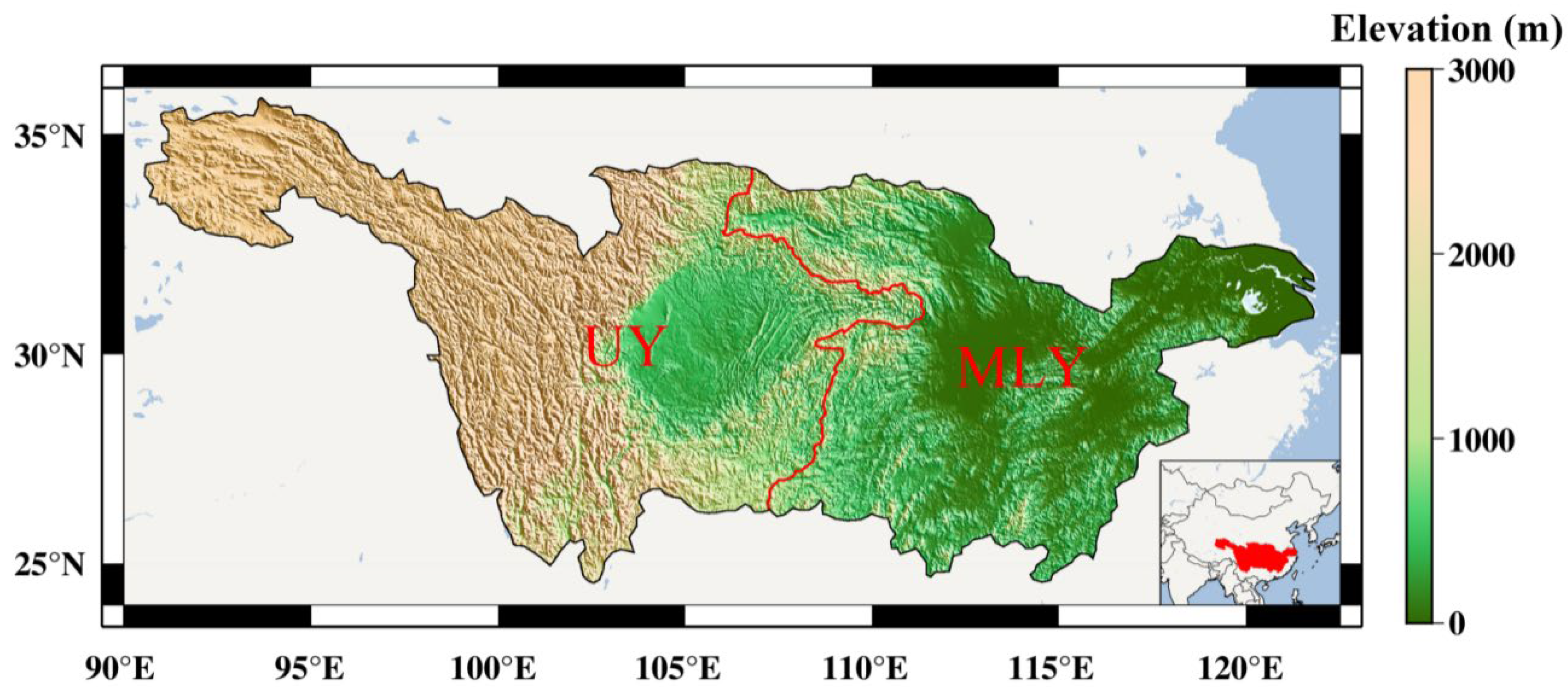
2.1. Study Area
2.2. Data
2.2.1. GRACE/GRACE-FO Data
2.2.2. Reconstructed TWSC Data
2.2.3. In Situ PPT Data
2.2.4. ET Data
2.2.5. GLDAS Model
2.2.6. Extreme Climate Index
3. Method
3.1. Different Datasets Fusion
3.2. The Correlation Coefficient and Delay Months
4. Results
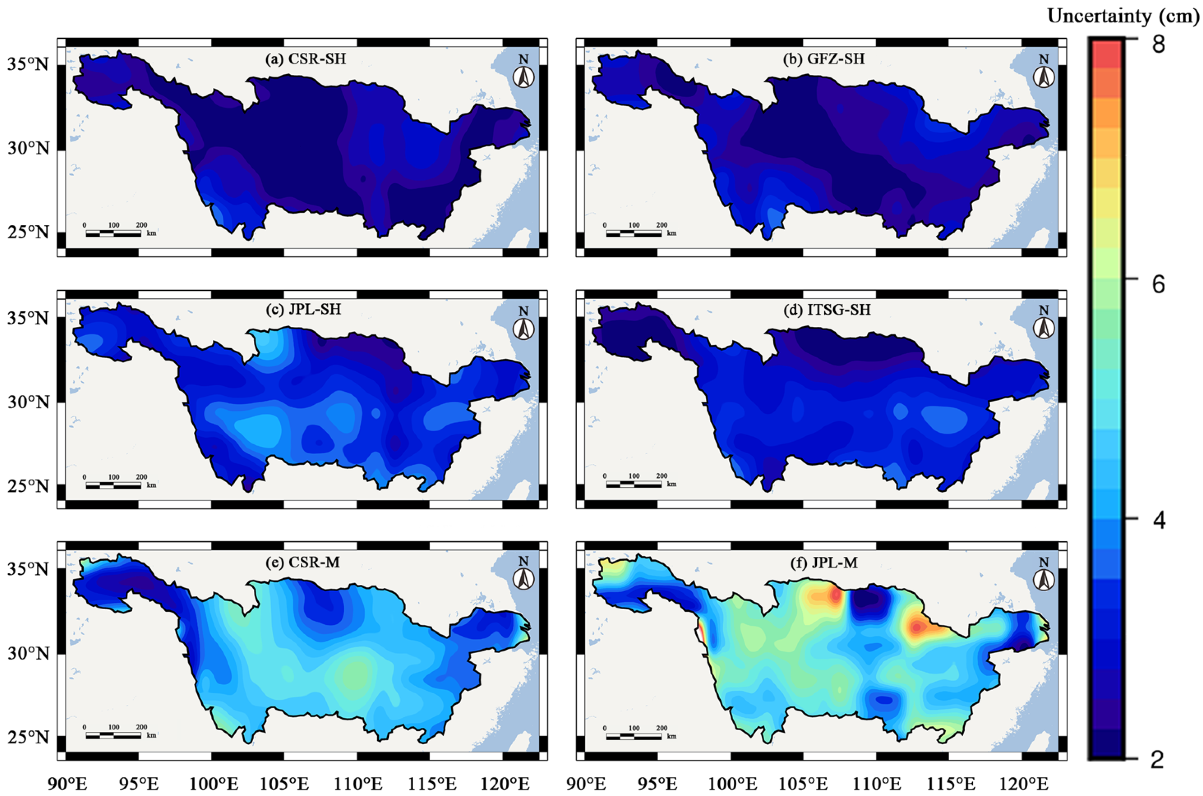
4.1. Data Fusion
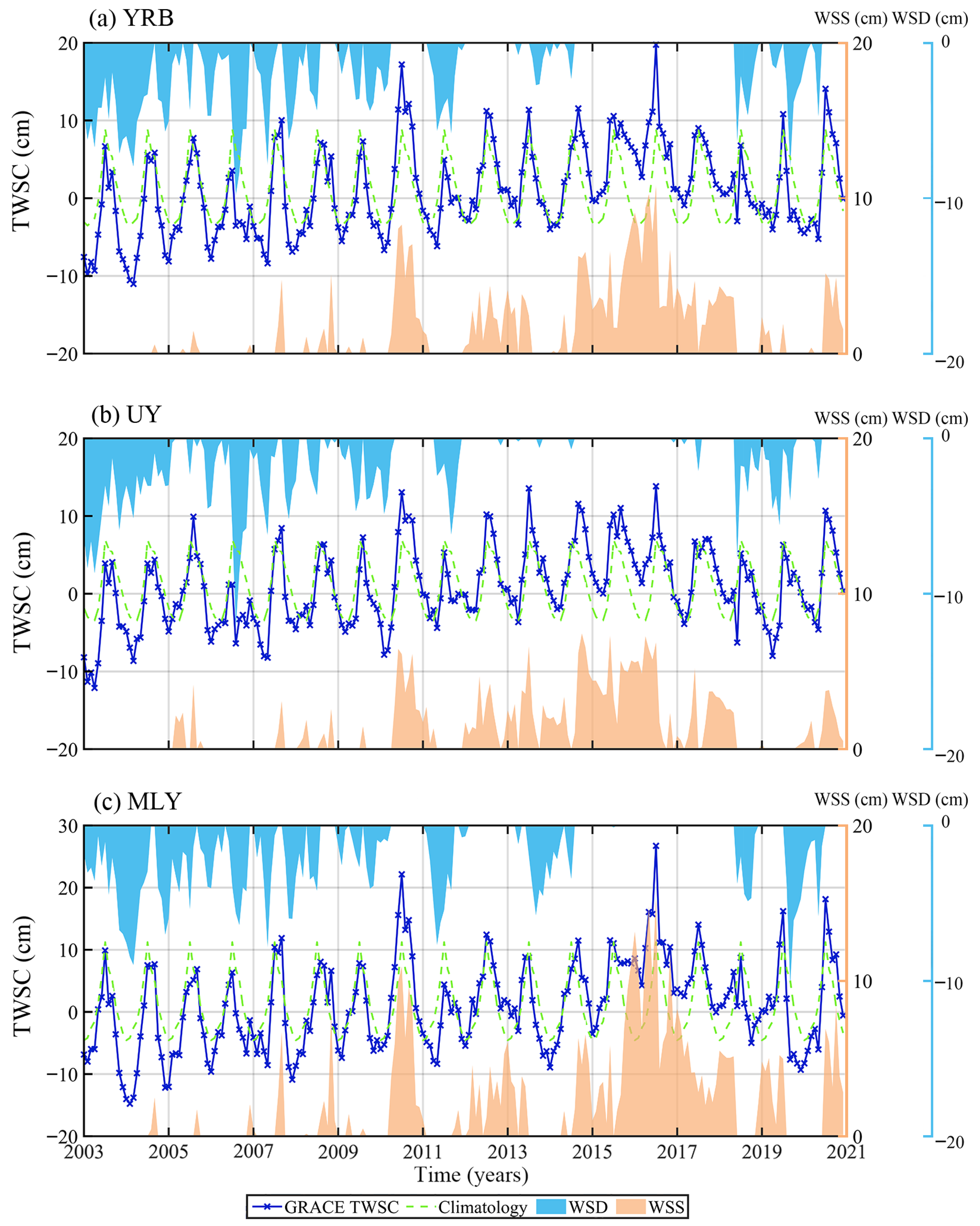
4.2. Droughts and Floods Events in the Study Regions
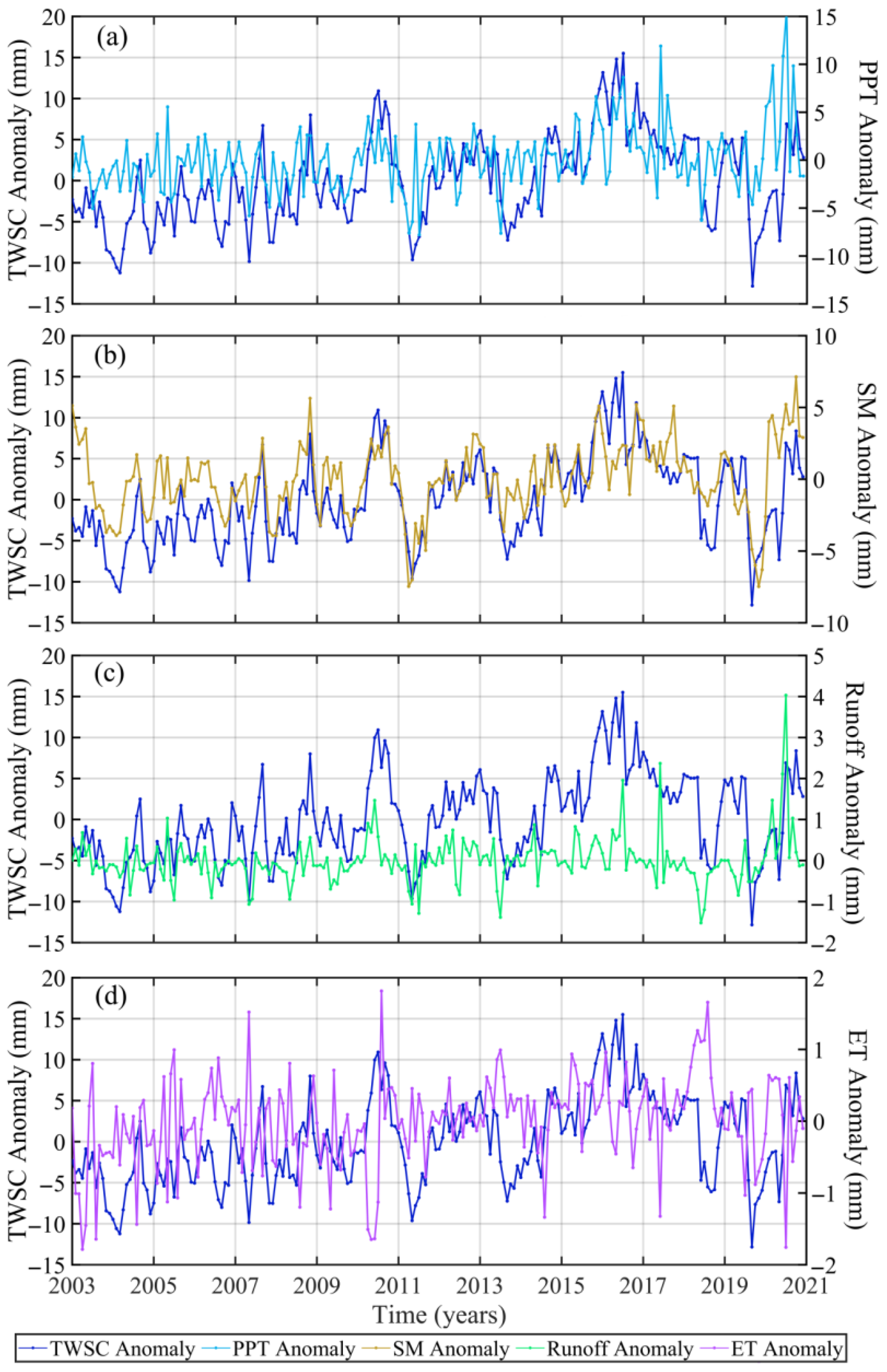
4.3. The Influence of Natural Factors on Drought and Floods in UY and MLY
4.4. The Influence of Extreme Climate on Drought and Floods in the UY and MLY
5. Discussion
6. Conclusions
Author Contributions
Funding
Institutional Review Board Statement
Informed Consent Statement
Data Availability Statement
Acknowledgments
Conflicts of Interest
References
- Barredo, J. Major flood disasters in Europe: 1950–2005. Nat. Hazards 2007, 42, 125–148. [Google Scholar] [CrossRef]
- Khan, A.; Zhao, Y.; Khan, J.; Rahman, G.; Rafiq, M.; UI Moazzam, M. Spatial and temporal analysis of rainfall and drought condition in Southwest Xinjiang in Northwest China, using various climate indices. Earth Syst. Environ. 2021, 5, 201–216. [Google Scholar] [CrossRef]
- Yin, J.; Gentine, P.; Zhou, S.; Sullivan, S.; Wang, R.; Zhang, Y.; Guo, S. Large increase in global storm runoff extremes driven by climate and anthropogenic changes. Nat. Commun. 2018, 9, 4389. [Google Scholar] [CrossRef] [PubMed] [Green Version]
- Cui, L.; Zhang, C.; Luo, Z.; Wang, X.; Li, Q.; Liu, L. Using the local drought data and GRACE/GRACE-FO data to characterize the drought events in Mainland China from 2002 to 2020. Appl. Sci. 2021, 11, 9594. [Google Scholar] [CrossRef]
- Jin, Z. Research on the Total Water Storage Change in the Yangtze River Basin and Its Connection with the Extreme Weather Events Using Time-Variable Gravity Data. Master’s Thesis, Wuhan University, Wuhan China, 2018. (In Chinese). [Google Scholar]
- Jiang, T.; Zhang, Q.; Zhu, D.; Wu, T.J. Yangtze floods and droughts (China) and teleconnections with ENSO activities (1470–2003). Quat. Int. 2006, 144, 29–37. [Google Scholar]
- Zhang, Q.; Xu, C.; Jiang, T.; Wu, Y. Possible influence of ENSO on annual maximum streamflow of the Yangtze River, China. J. Hydrol. 2007, 333, 265–274. [Google Scholar] [CrossRef]
- Wei, W.; Chang, Y.; Dai, Z. Streamflow changes of the Changjiang (Yangtze) River in the recent 60 year: Impacts of the East Asian summer monsoon, ENSO, and human activities. Quat. Int. 2014, 336, 98–107. [Google Scholar] [CrossRef]
- Li, J.; Mao, J.; Wu, G. A case study of the impact of boreal summer intraseasonal oscillations on Yangtze rainfall. Clim. Dyn. 2015, 44, 2683–2702. [Google Scholar] [CrossRef]
- Chen, X.; Zhang, L.; Zou, L.; Shan, L.; She, D. Spatio-temporal variability of dryness/wetness in the middle and lower reaches of the Yangtze River basin and correlation with large-scale climatic factors. Meteorol. Atmos. Phys. 2018, 3, 1–17. [Google Scholar] [CrossRef]
- Wahr, J.; Melenaar, M.; Bryan, F. Time variability of the Earth’s gravity field: Hydrological and oceanic effects and their possible detection using GRACE. J. Geophys. Res. Solid Earth 1998, 103, 30205–30229. [Google Scholar] [CrossRef]
- Han, S.; Shum, C.; Jekeli, C.; Alsdorf, D. Improved estimate of terrestrial water storage changes from GRACE. Geophys. Res. Lett. 2005, 32, 99–119. [Google Scholar] [CrossRef]
- Yao, C.; Luo, Z.; Wang, H.; Li, Q.; Zhou, H. GRACE-derived terrestrial water storage changes in the inter-basin region and its possible influencing factors: A case study of the Sichuan Basin, China. Remote Sens. 2016, 8, 444. [Google Scholar] [CrossRef] [Green Version]
- Chen, J.; Wilson, C.; Tapley, B.; Yang, Z.; Niu, G. 2005 drought event in the Amazon River basin as measured by GRACE and estimated by climate models. J. Geophys. Res. 2009, 114, B05404. [Google Scholar] [CrossRef]
- Cui, L.; Zhang, C.; Yao, C.; Luo, Z.; Wang, X.; Li, Q. Analysis of the influencing factors of drought events based on GRACE data under different climatic conditions: A case study in Mainland China. Water 2021, 13, 2575. [Google Scholar] [CrossRef]
- Zhang, Z.; Chao, B.; Chen, J.; Wilson, C. Terrestrial water anomalies of Yangtze River basin droughts observed by GRACE and connections with ENSO. Glob. Planet. Change 2015, 126, 35–45. [Google Scholar] [CrossRef]
- Li, Q.; Luo, Z.C.; Zhong, B.; Wang, H.H. Terrestrial water storage changes of the 2010 southwest China drought detected by GRACE temporal gravity field. Chin. J. Geophys. 2010, 56, 1843–1849. (In Chinese) [Google Scholar]
- Forootan, E.; Khaki, M.; Schumacher, M.; Wulfmeyer, V.; Mehrnegar, N.; van Dijk, A.; Brocca, L.; Frazaneh, S.; Akinluyi, F.; Rammillien, G.; et al. Understanding the global hydrological drought 2003–2016 and their relationship with teleconnections. Sci. Total Environ. 2019, 650, 2587–2604. [Google Scholar] [CrossRef] [Green Version]
- Reager, J.; Famiglietti, J. Global terrestrial water storage capacity and flood potential using GRACE. Geophys. Res. Lett. 2009, 36, L23402. [Google Scholar] [CrossRef] [Green Version]
- Chao, N.; Wang, Z. Characterized flood potential in the Yangtze River basin from GRACE gravity observation, hydrological model, and in-situ hydrological station. J. Hydrol. Eng. 2017, 22, 05017016. [Google Scholar] [CrossRef] [Green Version]
- Zhang, D.; Zhang, Q.; Wener, A.D.; Liu, X. Gravity based hydrological drought evaluation of the Yangtze River basin, China. J. Hydrometeorol. 2016, 17, 811–828. (In Chinese) [Google Scholar] [CrossRef]
- Swenson, S.; Chambers, D.; Whar, J. Estimating geocenter variations form a combination of GRACE and ocean model output. J. Geophys. Res. Solid Earth 2008, 113, 194–205. [Google Scholar] [CrossRef] [Green Version]
- Cheng, M.; Tapley, B.D. Variations in the Earth’s oblateness during the past 28years. J. Geophys. Res. 2004, 109, B09402. [Google Scholar]
- Cui, L.; Song, Z.; Luo, Z.; Zhong, B.; Wang, X.; Zou, Z. Comparison of terrestrial water storage changes derived from GRACE/GRACE-FO and Swarm: A case study in the Amazon River Basin. Water 2020, 12, 3128. [Google Scholar] [CrossRef]
- Zhong, Y.; Feng, W.; Zhong, M.; Ming, Z. Dataset of Reconstructed Terrestrial Water Storage in China Based on Precipitation (2002–2019); National Tibetan Plateau Data Center: Beijing, China, 2020. [Google Scholar] [CrossRef]
- Zhong, Y.; Feng, W.; Humphrey, V.; Zhong, M. Human-induced and climate-driven contributions to water storage variations in the Haihe River Basin, China. Remote Sens. 2019, 11, 3050. [Google Scholar] [CrossRef] [Green Version]
- Miralles, D.; Holmes, T.; de Jeu, R.; Gash, H.; Meesters, A.; Dolman, A. Global land surface evaporation estimated from satellite-based observations. Hydrol. Earth Syst. Sci. 2011, 15, 453–469. [Google Scholar] [CrossRef] [Green Version]
- Martens, B.; Miralles, H.; Lievens, H.; van der Schalie, R.; de Jeu, R.; Férnandez-Prieto, D.; Beck, H.; Dorigo, W.; Verhoest, N. GLEAM v3: Satellite-based land evaporation and root-zone soil moisture. Geosci. Model Dev. 2017, 10, 1903–1925. [Google Scholar] [CrossRef] [Green Version]
- Rodell, M.; Houser, P.; Jambor, U.E.A.; Gottschalck, J.; Mitchell, K.; Meng, C.; Arsenault, K.; Cosgrove, B.; Radakovich, J.; Bosilovich, M. The global land data assimilation system. Bull. Am. Meteorol. Soc. 2004, 85, 381–394. [Google Scholar] [CrossRef] [Green Version]
- Zhou, Z.; Xie, S.; Zhang, R. Historic Yangtze flooding of 2020 tied to extreme Indian Ocean conditions. Proc. Natl. Acad. Sci. USA 2021, 118, e2022255118. [Google Scholar] [CrossRef]
- Saji, N.; Goswami, B.; Vinayachandran, P.; Yamagata, T. A dipole model in the tropical Indian Ocean. Nature 1999, 401, 360–363. [Google Scholar] [CrossRef]
- Cui, L.; Yin, M.; Huang, Z.; Yao, C.; Wang, X.; Lin, X. The drought events over the Amazon River basin from 2003 to 2020 detected by GRACE/GRACE-FO and Swarm satellites. Remote Sens. 2022, 14, 2887. [Google Scholar] [CrossRef]
- Zhang, B.; Liu, L.; Yao, Y.; van Dam, T.; Khan, S. Improving the estimate of the secular variation of Greenland ice mass in the recent decades by incorporating a stochastic process. Earth Planet. Sci. 2020, 549, 116518. [Google Scholar] [CrossRef]
- Long, D.; Pan, Y.; Zhou, J.; Chen, Y.; Hou, X.; Hong, Y.; Scanlon, B.; Longuevergne, L. Global analysis of spatiotemporal variability in merged total water storage changes using multiple GRACE products and global hydrological models. Remote Sens. Environ. 2017, 192, 198–216. [Google Scholar] [CrossRef]
- Cui, L.; Zhu, C.; Wu, Y.; Yao, C.; Wang, X.; An, J.; Wei, P. Natural- and human-induced influences on terrestrial water storage change in Sichuan, Southwest China from 2003 to 2020. Remote Sens. 2022, 14, 1369. [Google Scholar] [CrossRef]
- Cui, L.; Luo, C.; Yao, C.; Zou, Z.; Wu, G.; Li, Q.; Wang, X. The influence of climate change on forest fires in Yunnan province, Southwest China detected by GRACE satellites. Remote Sens. 2022, 14, 712. [Google Scholar] [CrossRef]
- Chen, W.; Zhong, M.; Feng, W.; Zhong, Y.; Xu, H. Effects of two strong ENSO events on terrestrial water storage anomalies in China from GRACE during 2005–2017. Chin. J. Geophys. 2020, 63, 141–154. (In Chinese) [Google Scholar]
- Thomas, A.C.; Reager, J.T.; Famiglietti, J.S.; Rodell, M. A GRACE-based water storage deficit approach for hydrological drought characterization. Geophys. Res. Lett. 2014, 41, 1537–1545. [Google Scholar] [CrossRef] [Green Version]
- Cui, L. Research on Drought Events in Mainland China Using Satellite Time-Variable Gravity Field. Ph.D. Thesis, Wuhan University, China, 2021. (In Chinese). [Google Scholar]
- Chao, N.; Jin, T.; Cai, Z.; Chen, G.; Liu, X.; Wang, Z.; Yeh, P. Estimation of component contribution to total terrestrial water storage change in the Yangtze River basin. J. Hydrol. 2021, 595, 125661. [Google Scholar] [CrossRef]
- Yao, C. Natural- and Human-Induced Impacts on Regional Terrestrial Water Storage Changes from GRACE and Hydro-Meteorological Data. Ph.D. Thesis, Wuhan University, Wuhan, China, 2017. (In Chinese). [Google Scholar]
- Liu, Y.Q.; Ding, Y.H. Influence of ENSO events on weather and climate of China. J. Appl. Meteorol. Sci. 1992, 3, 473–481. [Google Scholar]
- Zhang, J. Research on the Impact of ENSO Events on the Climate of China. Master’s Thesis, Capital Normal University, Beijing, China, 2001. (In Chinese). [Google Scholar]
- Wang, J.; Liu, X.; Chen, H. Numerical study of the effects of spring IOD on East Asian summer monsoon. J. Trop. Meteorol. 2011, 27, 703–709. (In Chinese) [Google Scholar]
- Li, D.; Wang, Y.; Wei, D. The relationship between IOD and ENSO in the early autumn and its influence on the precipitation in the Yangtze River Basin in the following year. In Proceedings of the 2006 Annual Meeting of China Meteorological Society “Climate Change Its Mechanism and Simulation”, Chengdu, China, 25–27 October 2006; Chinese Meteorological Society: Beijing, China, 2006; pp. 1006–1017. (In Chinese). [Google Scholar]
- Li, C.; Mu, M. The influence of the Indian Ocean Dipole on atmospheric circulation and climate. Adv. Atmos. Sci. 2001, 18, 831–843. [Google Scholar]
- Anil, N.; Kumar, M.; Sajeev, R.; Saij, P. Role of distinct flavours of IOD events on Indian summer monsoon. Nat. Hazards 2016, 82, 1317–1326. [Google Scholar] [CrossRef]
- Qiu, Y.; Cai, W.; Guo, X.; Ng, B. The asymmetric influence of the positive and negative IOD events on China’s rainfall. Sic. Rep. 2014, 4, 6. [Google Scholar] [CrossRef] [PubMed] [Green Version]
- Liu, J.; Ma, Z.; Yang, S. The relationship between Indian Dipole and Huaxi Qiuyu. Plateau Meteorol. 2015, 34, 950–962. (In Chinese) [Google Scholar]
- Luo, J.; Zhang, R.; Behera, S.; Masumofo, Y.; Jin, F.; Lukas, F.; Yamagata, T. Interaction between El Niño and extreme Indian Ocean Dipole. J. Clim. 2010, 33, 726–742. [Google Scholar] [CrossRef]
- Hameed, S.; Jin, D.; Thilakan, V. A model for super El Niños. Nat. Commun. 2018, 9, 2528. [Google Scholar] [CrossRef] [Green Version]
- Wang, C. Three-ocean interactions and climate variability: A review and perspective. Clim. Dyn. 2019, 53, 5119–5136. [Google Scholar] [CrossRef] [Green Version]
- Zhang, R.; Tan, Y. El Niño and interannual variantion of the sea surface temperature in the tropical Indian Ocean. In Atmospheric and Oceanic Processes, Dynamics, and Climate Change; SPIE: Hangzhou, China, 2003; pp. 11–17. [Google Scholar]
- Behera, S.; Yamagata, T. Influence of the Indian Ocean Dipole on the Southern Oscillation. J. Meteorol. Soc. Jpn. 2003, 81, 169–177. [Google Scholar] [CrossRef]
- Annamalai, H.; Kida, S.; Hanfner, J. Potential impact of the tropical Indian Ocean-Indonesian Seas on El Niño characteristics. J. Clim. 2010, 23, 3933–3952. [Google Scholar] [CrossRef]
- Li, F.; Wang, Z.; Chao, N.; Song, Q. Assessing the influence of the Three Gorges Dam on hydrological drought using GRACE data. Water 2018, 10, 669. [Google Scholar] [CrossRef]


| Region | No. of Events | Time Span | Duration (Months) | Average WSD (km3) | Total WSD (km3) | Local Meteorological Data Validation (Y/N) |
|---|---|---|---|---|---|---|
| YRB 1,800,000 km2 | 8 | Jan-03 to Apr-05 | 28 | -75.60 | −2115.72 | N |
| Oct-05 to Jul 07 | 22 | −58.68 | −1290.42 | Y | ||
| Oct-07 to Jul 08 | 10 | −56.34 | −563.76 | Y | ||
| Jan-09 to Mar-10 | 15 | −40.32 | −604.08 | Y | ||
| Mar-11 to Dec-11 | 10 | −53.64 | −536.58 | Y | ||
| Aug-13 to Jan-14 | 6 | −25.38 | −152.64 | Y | ||
| Jun-18 to Dec-18 | 7 | −54.18 | −379.26 | Y | ||
| Apr-19 to Jun-20 | 15 | −37.44 | −562.14 | Y | ||
| UY 1,000,000 km2 | 7 | Jan-03 to Fre-05 | 26 | −70.92 | −1843.74 | N |
| Nov-05 to Jul 07 | 21 | −61.2 | −1286.82 | Y | ||
| Oct-07 to Jan-08 | 4 | −67.32 | −269.10 | Y | ||
| May-08 to Jul-08 | 3 | −52.02 | −155.88 | N | ||
| Feb-09 to Apr-10 | 15 | −45.18 | −677.52 | Y | ||
| May-11 to Nov-11 | 7 | −55.26 | −387.36 | Y | ||
| Jun-18 to Oct-19 | 17 | −44.82 | −763.20 | Y | ||
| MLY 800,000 km2 | 9 | Jan-03 to Jul-04 | 19 | −96.84 | −1840.68 | N |
| Oct-04 to Nov-06 | 26 | −71.28 | −1854.90 | Y | ||
| Feb-07 to Jul-07 | 6 | −68.94 | −413.10 | Y | ||
| Oct-07 to Jul-08 | 10 | −75.42 | −754.38 | Y | ||
| Jan-09 to Mar-10 | 15 | −36.36 | −546.48 | Y | ||
| Feb-11 to Sep-11 | 8 | −97.02 | −776.70 | Y | ||
| Jul-13 to Apr-14 | 10 | −69.84 | −697.86 | Y | ||
| Jun-18 to Nov-18 | 6 | −76.14 | −456.48 | Y | ||
| Aug-19 to Jun-20 | 11 | −90.36 | −993.24 | Y |
| Region | No. of Events | Time Span | Duration (months) | Average WSS (km3) | Total WSS (km3) | Local Meteorological Data Validation (Y/N) |
|---|---|---|---|---|---|---|
| YRB 1,800,000 km2 | 5 | Apr-10 to Feb-11 | 11 | 78.12 | 860.40 | Y |
| Jan-12 to Jul-13 | 19 | 41.58 | 790.02 | Y | ||
| Aug-14 to May-18 | 46 | 82.08 | 3778.38 | Y | ||
| Jan-19 to Mar-19 | 3 | 30.42 | 91.08 | Y | ||
| Jul-20 to Dec-20 | 6 | 64.80 | 388.98 | Y | ||
| UY 1,000,000 km2 | 7 | Mar-05 to May-05 | 3 | 37.62 | 112.68 | N |
| Feb-08 to Apr-08 | 3 | 17.46 | 52.20 | N | ||
| May-10 to Apr-11 | 12 | 61.56 | 738.90 | Y | ||
| Jan-12 to Sep-16 | 57 | 59.58 | 3393.90 | Y | ||
| Apr-17 to May-18 | 14 | 44.46 | 621.90 | Y | ||
| Nov-19 to Mar-20 | 5 | 13.68 | 68.22 | N | ||
| Jun-20 to Dec-20 | 7 | 38.34 | 268.20 | Y | ||
| MLY 800,000 km2 | 6 | Aug-08 to Dec-08 | 5 | 47.52 | 237.96 | N |
| Apr-10 to Jan-11 | 10 | 107.28 | 1073.16 | Y | ||
| Feb-12 to Mar-13 | 14 | 53.10 | 742.86 | Y | ||
| Aug-14 to May-18 | 46 | 105.12 | 4836.42 | Y | ||
| Dec-18 to Jul-19 | 8 | 66.24 | 529.20 | Y | ||
| Jul-20 to Dec-20 | 6 | 93.60 | 561.96 | Y |
| Hydrological Component | TWSC | PPT | SM | Runoff | ET |
|---|---|---|---|---|---|
| TWSC | 1 | 0.23 | 0.22 | 0.06 | 0.06 |
| PPT | 0.23 | 1 | 0.44 | 0.66 | −0.26 |
| SM | 0.22 | 0.44 | 1 | 0.35 | 0.16 |
| Runoff | 0.06 | 0.66 | 0.35 | 1 | −0.28 |
| ET | 0.06 | −0.26 | 0.16 | −0.28 | 1 |
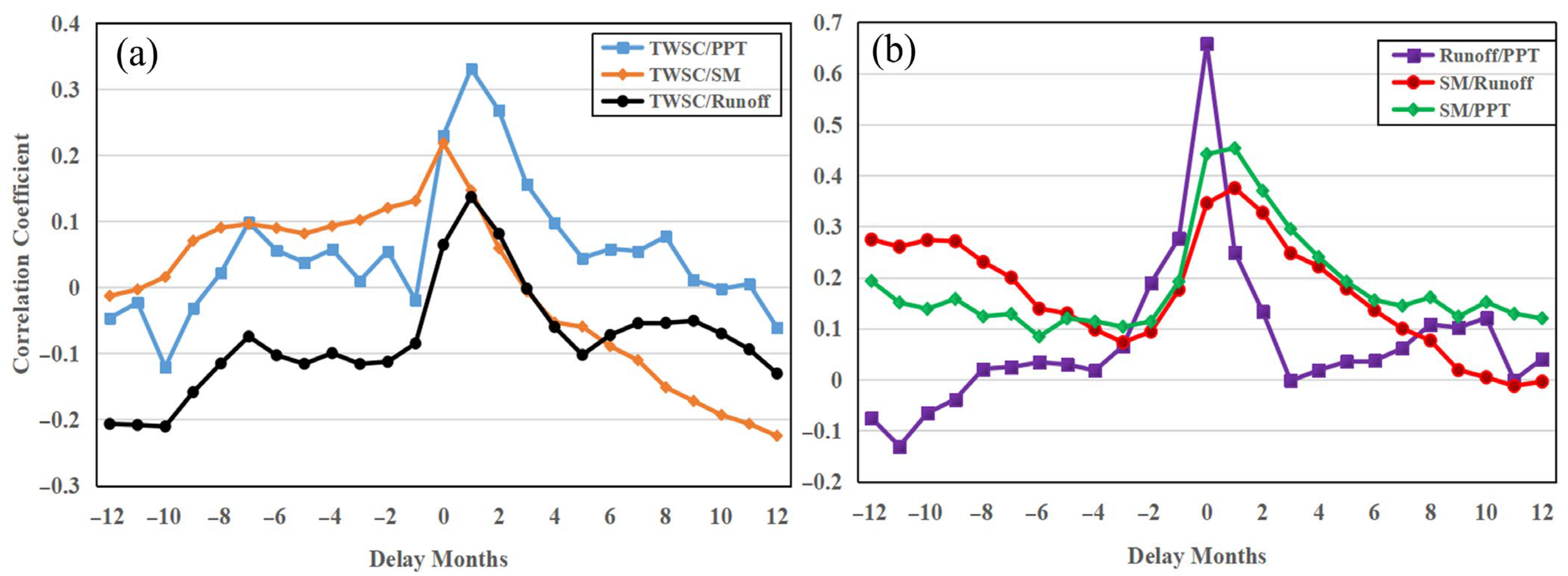
| Components | Correlation Coefficient | Time Delay Months |
|---|---|---|
| TWSC/PPT | 0.33 | 1 |
| TWSC/Runoff | 0.14 | 1 |
| TWSC/SM | 0.22 | 0 |
| SM/PPT | 0.45 | 1 |
| Runoff/PPT | 0.66 | 0 |
| SM/Runoff | 0.38 | 1 |
| Hydrological Component | TWSC | PPT | SM | Runoff | ET |
|---|---|---|---|---|---|
| TWSC | 1 | 0.41 | 0.67 | 0.37 | 0.03 |
| PPT | 0.41 | 1 | 0.47 | 0.80 | −0.33 |
| SM | 0.68 | 0.47 | 1 | 0.47 | −0.03 |
| Runoff | 0.37 | 0.80 | 0.47 | 1 | −0.40 |
| ET | 0.03 | −0.33 | −0.03 | −0.40 | 1 |
| Components | Correlation Coefficient | Delay Months |
|---|---|---|
| TWSC/PPT | 0.51 | 1 |
| TWSC/runoff | 0.38 | 1 |
| TWSC/SM | 0.67 | 0 |
| SM/PPT | 0.52 | 1 |
| Runoff/PPT | 0.80 | 0 |
| SM/Runoff | 0.47 | 0 |
| ENSO Events | Disaster | |||
|---|---|---|---|---|
| Type | Time Span | Y/N | Type | Location |
| El Niño | Aug-04 to Jan-05 | Y | Floods | UY |
| El Niño | Sep-06 to Jan-07 | N | - | - |
| La Niña | Aug-07 to May-08 | Y | Droughts | UY, MLY |
| El Niño | Jul-09 to Apr-10 | Y | Floods | UY, MLY |
| La Niña | Jun-10 to May-11 | Y | Droughts | MLY |
| La Niña | Aug-11 to Fre-12 | Y | Droughts | UY, MLY |
| El Niño | Apr-15 to Apr-16 | Y | Floods | UY, MLY |
| La Niña | Sep-17 to Mar-18 | Y | Droughts | UY, MLY |
| El Niño | Oct-18 to Jun-19 | Y | Floods | MLY |
| IOD Events | Disaster | |||
|---|---|---|---|---|
| Type | Time Span | Y/N | Type | Location |
| Negative | Apr-04 to Aug-04 | Y | Droughts | UY, MLY |
| Negative | Nov-04 to Mar-05 | Y | Droughts | UY, MLY |
| Negative | Jun-05 to Mar-06 | Y | Droughts | UY, MLY |
| Positive | Jun-06 to Nov-07 | Y | Floods | UY, MLY |
| Positive | May-08 to Oct-08 | Y | Floods | UY, MLY |
| Positive | Dec-08 to Jun-09 | Y | Droughts | MLY |
| Positive | Sep-09 to May-10 | Y | Floods | UY, MLY |
| Positive | Jun-11 to Nov-11 | Y | Droughts | UY, MLY |
| Positive | Jun-12 to Mar-13 | Y | Floods | UY, MLY |
| Negative | Apr-13 to Oct-13 | Y | Floods | UY |
| Positive | Apr-15 to Jan-16 | Y | Floods | UY, MLY |
| Negative | May-16 to Jan-17 | Y | Floods | UY, MLY |
| Positive | Feb-17 to Dec-17 | Y | Floods | UY, MLY |
| Positive | May-18 to Jul-20 | Y | Floods | UY, MLY |
| Variables | Correlation Coefficients | Delay Months | ||
|---|---|---|---|---|
| UY | MLY | UY | MLY | |
| ENSO vs. TWSC | 0.39 | 0.50 | 8 | 8 |
| ENSO vs. PPT | 0.31 | 0.68 | 6 | 5 |
| ENSO vs. SM | 0.42 | 0.42 | 11 | 9 |
| DMI vs. TWSC | 0.19 | 0.09 | 6 | 6 |
| DMI vs. PPT | 0.49 | 0.28 | 5 | 5 |
| DMI vs. SM | 0.27 | 0.10 | 11 | 8 |
Publisher’s Note: MDPI stays neutral with regard to jurisdictional claims in published maps and institutional affiliations. |
© 2022 by the authors. Licensee MDPI, Basel, Switzerland. This article is an open access article distributed under the terms and conditions of the Creative Commons Attribution (CC BY) license (https://creativecommons.org/licenses/by/4.0/).
Share and Cite
Cui, L.; He, M.; Zou, Z.; Yao, C.; Wang, S.; An, J.; Wang, X. The Influence of Climate Change on Droughts and Floods in the Yangtze River Basin from 2003 to 2020. Sensors 2022, 22, 8178. https://0-doi-org.brum.beds.ac.uk/10.3390/s22218178
Cui L, He M, Zou Z, Yao C, Wang S, An J, Wang X. The Influence of Climate Change on Droughts and Floods in the Yangtze River Basin from 2003 to 2020. Sensors. 2022; 22(21):8178. https://0-doi-org.brum.beds.ac.uk/10.3390/s22218178
Chicago/Turabian StyleCui, Lilu, Mingrui He, Zhengbo Zou, Chaolong Yao, Shengping Wang, Jiachun An, and Xiaolong Wang. 2022. "The Influence of Climate Change on Droughts and Floods in the Yangtze River Basin from 2003 to 2020" Sensors 22, no. 21: 8178. https://0-doi-org.brum.beds.ac.uk/10.3390/s22218178